Behavior Research Methods 2006, 38 (1), 123-133
Modeling visual attention SØREN KYLLINGSBÆK University of Copenhagen, Copenhagen, Denmark Quantitative modeling of psychological data is both technically and mathematically challenging. The present article introduces a user friendly and flexible program package that enables quantitative fits of Bundesen’s (1990) theory of visual attention to behavioral data from whole and partial report experiments. The program package is based on new computational formulas that are more general than previous ones and has already been used successfully in a number of neuropsychological investigations of attentional disorders, such as visual neglect and simultanagnosia. A clinical version of the program package is currently under development.
Visual attention is a major field within cognitive psychology, with many articles published every year (e.g., Bundesen & Habekost, 2005). Bundesen (1990; see also Bundesen, 1998; Bundesen, Habekost, & Kyllingsbæk, 2005) has proposed a computational theory of visual attention (TVA) that, contrary to most other theories in the field, yields direct quantitative predictions in different paradigms (e.g., visual search and whole and partial report). Lately, the model has been applied to data from neuropsychological patients with attentional deficits, such as visual neglect (Duncan et al., 1999), simultanagnosia (Duncan et al., 2003), and subclinical attentional symptoms following a frontal-subcortical lesion (Habekost & Bundesen, 2003). The model has also been integrated with theories of memory, categorization, and executive function (see Logan, 2002; Logan & Gordon, 2001; see also Logan, 1996). Although quantitative modeling of data from psychological experiments is a promising line of research, it is both mathematically and technically challenging. Typically, the mathematical algorithms used to estimate the model have to be reevaluated and reprogrammed even when minor changes to the experimental paradigm are introduced. This article presents a new generalized mathematical framework that extends the derivations of TVA presented previously (see Bundesen, 1990; Duncan et al., 1999; Shibuya & Bundesen, 1988). Furthermore, the generalized mathematical framework is implemented in
This research was supported by grants from the Carlsberg Foundation, the Danish Research Council for the Humanities, and the Danish Strategic Research Council. I thank Thomas Habekost for providing the exemplary data set used in the article. I also thank Thomas Habekost, Claus Bundesen, and Matthieu Dubois for helpful comments on earlier versions of the manuscript. Correspondence concerning this article should be addressed to S. Kyllingsbæk, Center for Visual Cognition, Department of Psychology, University of Copenhagen, Linnésgade 22, DK-1361 Copenhagen K, Denmark (e-mail:
[email protected]). Note—The author has a financial interest in some or all of the software presented in this article. —Editor
a user friendly program package that enables experimenters without a mathematical and technical background to model data from whole and partial report experiments based on Bundesen’s (1990) TVA. A Theory of Visual Attention TVA is a combined theory of recognition and selection. Whereas many theories of visual attention separate the two processes both in time and in representation, TVA instantiates the two processes in a unified mechanism implemented as a race model of both selection and recognition. In other words, when an object in the visual field is recognized, it is also selected at the same time, and vice versa. By the unification of selection and recognition, TVA tries to resolve the long-standing debate of early versus late selection. The first position claims that selection occurs prior to recognition (e.g., Broadbent, 1958), and the other that recognition is the precursor for selection (e.g., Deutsch & Deutsch, 1963). According to TVA, elements in the visual field are processed in parallel. Visual processing is a two-stage process consisting of (1) an initial match of the visual impression with visual long-term memory (VLTM) representations, followed by (2) a selection/recognition race for representation in visual short-term memory (VSTM). Note that the initial match in VLTM does not imply recognition. Thus, after the match, both the strength of evidence that a given letter is a C and the strength of evidence that the letter is a G may be positive. Only after the recognition/selection race is the letter recognized—that is, categorized as either a C or a G. The first stage: Computation of η values. According to TVA, visual processing starts with a massively parallel comparison (matching) between objects in the visual field and representations in VLTM. This process is capacity unlimited, in the sense that the time it takes is independent of the number of objects in the visual field. The end result of the matching process is the computation of η(x,i) values (evidence values), each measuring the degree of match between a given object x and a long-term memory representation (category) i.
123
Copyright 2006 Psychonomic Society, Inc.
124
KYLLINGSBÆK
The η values are affected by the visibility (e.g., contrast) of the visual stimuli, as well as by the degrees of pattern match between the stimuli and the representations in VLTM. The latter are affected by learning, which may lead to change in or even development of new representations in VLTM. Thus, one may, for instance, learn to read one’s own name more quickly than other first names (see Bundesen, Kyllingsbæk, Houmann, & Jensen, 1997). Altogether, η values are affected only by the objective properties of the visual environment and the VLTM of the perceiver, but not by the subjective properties, such as selection criterion or categorization bias. The second stage: The race. Different categorizations of the objects in the visual field compete for entrance into VSTM in a stochastic race process. The capacity of VSTM is limited to K elements, where K typically takes on a value around 4. Categorizations of the first K visual objects to finish processing are stored in VSTM (the first K winners of the race). Categorizations from other elements are lost but may give rise to priming effects and other subliminal phenomena. Note that categorizations from elements already represented by other categorizations may freely enter VSTM even though it is full, so that there is no room for categorizations of other objects. Thus, VSTM is limited with respect to the number of elements of which categorizations may be stored, not with respect to the number of categorizations of the elements represented in the store (see Duncan, 1984; Luck & Vogel, 1997; but see also Wheeler & Treisman, 2002). As was stated above, visual objects are processed in parallel in TVA. Furthermore, the theory assumes independence between visual categorizations of different objects and between different types of categorizations of the same object. Consider the situation in which only two objects are present in the visual field and the two objects are to be judged with respect to color and shape. Given that VSTM capacity is larger than two, VSTM is not a limiting factor. If attentional parameters are kept constant, TVA predicts that the probability that the first object will be correctly categorized with respect to color is independent of whether the object is correctly categorized with respect to shape and independent of whether the other object is correctly categorized with respect to color or shape. Strong evidence for independent processing both within and between objects when VSTM is not a limiting factor has been found by Bundesen, Kyllingsbæk, and Larsen (2003). To determine the rate of processing of each categorization of an element, the η values are combined with two types of subjective values, pertinence and bias. As has been suggested by Broadbent (1971), two different attentional mechanisms are necessary for adequate behavior: one for filtering (based on pertinence) and one for pigeonholing (based on bias). For example, if participants are to report the identity of black target letters among white distractor letters, the white distractors must be filtered out, and the black targets must be categorized with respect to letter identity. In TVA terms, pertinence should be high for black and low for white stimuli, and bias should be high
for letter identities and low for all the other categories. In other words, the filtering is based on color, and pigeonholing on the letter identity. The rate of processing v(x,i) of a categorization in the race is given by two equations. By Equation 1, wx v ( x , i ) = η ( x , i ) βi , (1) ∑ wz z ∈S
where η(x,i) is the strength of the sensory evidence that element x belongs to category i, βi is the perceptual bias associated with i, S is the set of elements in the visual field, and wx and wz are attentional weights for elements x and z. Thus, the rate of processing is determined as the strength of the sensory evidence that object x is of category i weighted by the bias toward making categorizations of type i and by the relative attentional weight of object x (given by the ratio of wx over the sum of the attentional weights of all objects in the visual field). The attentional weights are, in turn, given by wx =
∑ η ( x, j ) π j ,
(2)
j ∈R
where R is the set of perceptual categories, η(x, j) is the strength of the sensory evidence that element x belongs to category j, and πj is the pertinence (priority) value associated with category j. The distribution of pertinence values defines the selection criteria at any given point in time (filtering). By Equation 2, the attentional weight of object x is a weighted sum of pertinence values, where each pertinence value πj is weighted by the degree of evidence that object x actually is a member of category j. In most experimental setups, η, β, and π values can be assumed to be constant during the stimulus presentation, which implies that v values are also constant (see Equations 1 and 2). The v values are defined as rate parameters in the encoding process. When the v values are constant, the time taken to encode a categorization may be assumed to be exponentially distributed (see Bundesen, 1990, p. 529), with the probability density function given by ⎧⎪0 f (t ) = ⎨ ⎩⎪v ( x, i ) exp ⎡⎣ − v ( x, i ) ( t − t0 ) ⎤⎦
for t < t0 for t ≥ t0 (3)
and the probability distribution function given by t
F (t ) =
∫ f (t ′ ) dt ′ 0
⎧⎪0 =⎨ ⎩⎪1 − exp ⎡⎣ − v ( x, i ) ( t − t0 ) ⎤⎦
for t < t0 for t ≥ t0
.
(4)
The distribution function F(t) yields the probability that processing is completed before time t. The density function, on the other hand, describes the probability density at any given time t. Thus, the distribution function F(t) may be derived by integration of the density function f(t) from 0 to t, as shown in Equation 4 (see Ross, 2000, chap. 4). Equations 3 and 4 state that processing does not begin until time t0, the threshold for conscious perception. Af-
MODELING VISUAL ATTENTION terward, processing follows the exponential distribution shifted in time by t0. Typically, t0 is estimated in the range of 20 msec in normal healthy participants. Joint probabilities. Until now, the focus has been on categorizations of individual items. As was stated above, processing of different categorizations are thought to be parallel and mutually independent, according to TVA. Thus, calculation of the joint probabilities follows easily from the fact that the joint probability of independent random variables is given by the product of the marginal probabilities of the single events (i.e., categorizations in the present context). Consider first a simple case of whole report (report of all stimuli in the display; see the detailed description below) in which the VSTM capacity given by parameter K is not a limiting factor. Let S be the set of stimuli presented, and let R be the set of stimuli correctly reported by the participant. The joint probability of reporting R when S is presented is given by Ps ( R) =
∏ Fi (τ ) ∏
i ∈R
j ∈S − R
⎡1 − Fj (τ ) ⎤ , ⎣ ⎦
(5)
where τ is equal to t ⫺ t0 (the effective exposure duration), Fi is the probability distribution function of reporting item i in R, and 1 ⫺ Fj is the probability of not reporting item j in the set of items outside R. Matters are more complicated when the VSTM capacity K is a limiting factor. This is the case when the number of reported items is equal to the limit of VSTM and the number of presented items exceeds the limit—that is, when K ⫽ n(R) and K ⬍ n(S), where n(R) and n(S) are the numbers of elements in R and S, respectively. Then, processing times of the categorizations are still mutually independent, but only categorizations from the first K stimuli will be included in R. The joint probability is then given by Ps ( R) =
τ
∑ ∫ f i (t ) ∏
i ∈R 0
j ∈R −{i}
F j (t )
∏
k ∈S − R
⎣⎡1 − Fk (t ) ⎤⎦ dt . (6)
The rationale behind Equation 6 is that each item i in R may be the last to enter VSTM, thus effectively preventing other items from entering. Integration is done on the probability density distribution that all the other items in R indexed by j have finished processing at time t, that all items in the set S ⫺ R (the losers of the race) have not yet finished processing, and that item i finishes processing at time t. In the Appendix of the present article, new generalized closed-form versions of Equations 5 and 6 are derived. The formulas extend previous derivations (cf. Bundesen, 1990; Duncan et al., 1999; Shibuya & Bundesen, 1988). Similar generalized formulas are also derived for the partial report paradigm. The closed-form formulas from the Appendix are implemented in the program package described below. The Paradigms: Whole and Partial Report The main paradigms modeled by TVA have been the whole and partial report paradigms introduced by Sper-
125
ling (1960) as measures of both processing and short-term memory capacity. In whole report, the task is to report the identity of as many as possible of the presented stimuli. Typically, unrelated letters are presented, and both the number of letters presented and the exposure duration are varied. The letter display may be followed either by a masking display, which controls the effective exposure duration, or by a blank display, which enables the participant to take advantage of the decaying image of the stimuli. This will result in an increase of the effective exposure duration beyond the physical duration of the stimuli. The effect of the decaying visual image is modeled as an exponential decay of the v parameters. The effect of the decay is estimated by parameter μ, which measures the prolongation of the effective exposure duration resulting from the decaying image (see Bundesen, 1990, pp. 528–529). In partial report, the stimuli are divided into two classes: targets and distractors. The task is to report as many of the target stimuli as possible, while ignoring the distractors. The selection criterion is defined as the stimulus dimension distinguishing the two classes of stimuli. The selection criterion could, for example, be color, and the targets could be red letters presented among green distractor letters. As can be seen from Equation 1, the absolute value of the attentional weight of an item is not important, due to the ratio of attentional weights in the equation. Consequently, the attentional weights may be normalized without any loss of generality, so that the target with the largest weight is assigned an attentional weight of 1. Rather than representing attentional weights of distractors directly, the weight of a distractor (wD) relative to the weight of a target (wT) at a given location is estimated by parameter α ⫽ wD /wT. An α value of 0, then, means perfect selection, and an α value of 1 conversely means no selectivity for targets rather than for distractors. The impact of distractors may vary considerably across different types of selection criteria—for example, being very small when color is used (α value close to 0; see Bundesen, Pedersen, & Larsen, 1984; Bundesen, Shibuya, & Larsen, 1985) and significantly larger when using alpha-numeric class (i.e., reporting letters among digit distractors; α value close to 0.50; see Shibuya & Bundesen, 1988). However, estimates of α values inherently tend to vary relatively strongly even when based on large data sets. This is because α is the ratio formed by dividing the weight of a distractor by the weight of a target. If both weights are positive but close to zero (as may be found, e.g., at locations in the neglected hemifield in patients with unilateral neglect), a small variability in the estimates for the weights causes a large variability in the estimate of α. A Program Package for Estimating the TVA Model The program package for fitting the TVA model to whole and partial report data consists of two separate programs: MakeModel for setting up the specific model to be estimated and WinTVAFit for running the estimation
126
KYLLINGSBÆK
process that combines the specified model with the observed data. The program package also contains a manual explaining how the programs are used and exemplary data sets that may be used for tutorials.1 Specifying the model. Setting up the model to be estimated happens in three steps: (1) choice of paradigm, (2) specification of the number of different parameters to be estimated, and finally, (3) specification of the initial values and limits of the parameters, as well as linking the parameters to specific experimental conditions and display locations. The initial specification of the experimental paradigm includes the overall decision between whole and partial report. Furthermore, the number of different experimental conditions (trial types) is specified, along with the number of possible display locations used. The display size and exposure duration may be chosen as either variable or constant. However, both cannot be constant at the same time. This choice will have implications as to which parameters may be estimated (see Table 1). If the display size is constant, it will not be possible to separate the attentional weights in Equation 1 from the complex s ⫽ ηβ. The reason why s and the attentional weights may not be separated is that they are not varied independently of one another when the display size is kept constant across the different experimental conditions. Thus, if display size is chosen to be constant, only v values for the display locations will be estimated (see Equations 1–4). If, on the other hand, exposure duration is kept constant while the display size is varied, it is not possible to separate s from the effective exposure duration, indirectly represented by the threshold for conscious perception t0, and the effect of the decaying image in nonmasked displays represented by the μ parameter. Then only the total amount of processing, A ⫽ s (t ⫺ t0 ⫹ μ) (the accumulated number of categorizations made at each display location), may be estimated, along with differences in attentional weights. Finally, the maximum score—that is, the maximum number of correctly reported items—may be thresholded. This threshold is used when a small number of high scores are observed, usually less than 5% of the total number of trials. These high scores may be due to “lucky guesses,” where the participant incidentally reports a large number of items correctly and thus exceeds the usual limit of the VSTM capacity K. After the paradigm is specified, a decision is made concerning the number of parameters to be estimated.
Table 1 Possible Parameter Combinations to be Estimated in Different Whole and Partial Report Paradigms Display Size Exposure Duration Constant Varied Constant – A, wT, K, α Varied v, t0, μ, K, α s, t0, μ, wT, K, α Note—wT represents the attentional weight of a target. α values can be fitted only in partial report paradigms.
Parameters K, t0, and μ are limited from 1 to the number of experimental conditions. The VSTM capacity K, for example, is usually thought to be constant across experimental conditions; thus, only a single K parameter should be estimated. But when neurological patients with unilateral lesions are studied, it may be necessary to estimate two K parameters, one for each hemifield. In this case, experimental conditions should be separable in terms of lateralization of the stimuli, so that stimuli are presented either to the left or to the right. Although VSTM capacity is assumed to take on an integer value in any given moment, it may vary somewhat across time in a participant. Consequently, parameter K is estimated as a probability mixture. Thus, an estimate of K at 3.76 represents a probability mixture where K is 4 with a probability of .76 and 3 with a probability of 1 ⫺ .76 ⫽ .24. Parameters relating to the processing rates of the single stimuli—that is, v, s, or A values, as well as attentional weights and α values—are limited from 1 to the number of possible display locations. In the initial estimations of the TVA model (e.g., Shibuya & Bundesen, 1988), these values were estimated as constant across all possible display locations, which is a good approximation for normal healthy participants who are told to pay equal attention to all locations in the display. In this case, it is sufficient to estimate only a single processing capacity parameter and a single α value when fitting partial report data. However, when patients are tested, the difference in parameter estimates across different display locations is often essential. For example, when patients suffering from visual neglect are studied, it may be important to estimate visualprocessing parameters v, s, or A, as well as attentional weights and α values, for each hemifield. It may even be necessary to estimate parameters for each display location, if the patient is suspected to suffer from scotomas leading to reduction in processing at specific locations in the display. One should be cautious, though, about specifying a model with too many parameters. This may lead to overfitting, where the flexibility of the model results in a fit that is too dependent on the noise in the data, rather than a model that captures only the relevant structure. A formal way of testing whether the model is overfitting the data is to split the data set in a learning set and a test set. The model is fitted to the learning set, and the predicted values are then compared with the observed values in the test set, yielding an error estimate. By using different models with increasing numbers of parameters, a learning curve may be plotted comparing number of parameters with the error estimate. The learning curve will typically be U-shaped, having high values when the number of parameters is small (the model is too simple to capture the pattern in the data) and when the number of parameters is too high (overfitting). Thus, the learning curve will have a minimum indicating the optimal number of parameters (e.g., Bishop, 2003, chap. 1). The last step in specifying the model is to set up initial parameter values and limits used in the estimation pro-
MODELING VISUAL ATTENTION cedure. The estimation procedure is an iterative search for the optimal set of parameters within the multidimensional parameter space. The limits for each parameter are introduced in order to prevent the search algorithm from running astray. An optimal choice of the initial parameter values used as the starting point for the search will further facilitate the estimation process. With this in mind, it may be a good idea to try different initial parameters and fit the model several times, to make sure that the final parameter estimates are stable. After the limits and initial value have been set, the parameters are linked to specific experimental conditions or display locations. If a parameter value is known in advance (e.g., estimated from another data set of the same participant), it may be fixed and treated as a constant in the model, equal to the initial value of the parameter. Finally, the model is saved as an ASCII text file, which will later be used by the estimating program WinTVAFit, in combination with the data file. Model files may also be loaded into the MakeModel program for modification. Fitting the model to the observed data. Before the model is estimated, the raw data have to be transformed to a specific format (see Table 2). The estimation process is iterative and based on the maximum likelihood of the model across individual trials. The optimization algorithm used is the so-called Powell algorithm described in Press, Teukolsky, Vetterling, and Flannery (2002, pp. 417–424). The step size and the optimization threshold in terms of both the number of iterations and the minimum change in the optimization function may be set before the estimation process is started. Finally, it is possible to estimate the variation in the parameter estimates, using the bootstrap method suggested by Efron and Tibshirani (1993; see details below). The estimation process may then be started, using the model and data file. It will run until either the change in the optimization function is less than the specified threshold or the maximum number of iterations has been reached. If bootstrap estimation has been chosen, the estimation process will be repeated until the number of bootstrap repetitions specified has been reached (see the detailed description below). The estimation procedure may be run in batch mode if data from more than 1 participant have to be modeled. A model is estimated for each data file in succession. The model file used for each data file may be individually specified. The output file. The result of the estimation process is written to an output file in ASCII format, which may easily be imported into standard spreadsheet programs. The first part of the output file contains the parameter estimates and a table of the observed and predicted position probabilities for each experimental condition. The position probabilities represent the probability that an item will be reported correctly at a certain display location. The correlation coefficient is given as an estimate of the correspondence between the observed and the predicted position probabilities. In a second table, observed and predicted score distributions are given for the different experimental conditions.
127
Table 2 Data Format Used by the WinTVAFit Program: Example Data Set From a Partial Report Experiment With 10 Possible Stimulus Locations and Constant Exposure Duration at 10 msec 300 4 10 00AMJ00000 0000000000 AJ 3 10 0000PB0AYN 0000000000 BYAM 2 10 00000AH00J 0000000EP0 AH 5 10 00000E0M0B 0000000000 EB 1 10 0NR0K00000 E00X000000 X 4 10 AEP0000000 0000000000 A 5 10 000000E0JL 0000000000 EJL 3 10 TNP0R00H00 0000000000 – 1 10 LM00H00000 00SJ000000 LH 2 10 00000LW00Z 0000000MB0 LW 1 10 0YB0T00000 J00R000000 Y 2 10 00000Z0EH0 000000B00Y ZEH 3 10 WS0HB00R00 0000000000 WR 4 10 LS0J000000 0000000000 LSJ 5 10 00000A0K0L 0000000000 AKL 3 10 0N0J000MPH 0000000000 NP 5 10 00000HLP00 0000000000 HLP 4 10 JX00A00000 0000000000 JXA 2 10 00000Z00LT 000000WM00 TX 1 10 Z00WK00000 0HN0000000 ZK ... Note—First row indicates the total number of trials in the data file. Each following row represents a trial. The columns represent (1) experimental conditions, (2) exposure duration in milliseconds, (3) targets at each of 10 display locations (a zero indicates no target at that location), (4) distractors at each of the 10 display locations, and (5) the reported items. A dash indicates no reported items.
The score distribution is the distribution of probabilities of reporting 0, 1, 2, . . . items correct in a given experimental condition. An estimate of the correspondence between the observed and the predicted score distributions is given by Kolmogorov–Smirnov D values for each condition, as well as by the mean Kolmogorov–Smirnov D across conditions. The Kolmogorov–Smirnov D measures the maximal difference between a predicted and an observed cumulative frequency distribution, and the predicted distribution represents what would be expected given the H0 hypothesis (see Siegel & Castellan, 1988, pp. 51–55). If bootstrap estimation has been chosen, the bootstrap estimates of the parameters will be given at the end of the file. The parameter estimates from each bootstrap iteration will be represented in a single line. From these values, the bootstrap estimate of the variation in each parameter may be calculated as the sample standard deviation of the bootstrap estimates for each parameter. The bootstrap method. As was described above, the TVA model provides the formulas for estimating both processing and short-term memory capacities. However, reliability estimates of the parameters are not explicitly derived. Thus, when a processing rate of 4.2 elements/sec has been estimated at a given location in the visual field, one does not know whether the true value is 3, 6, or even 12 elements/sec. The straightforward way to estimate the reliability of the parameters would be to repeat the experiment many times. The model may then be estimated for each repetition of the experiment, and the standard deviation of the
KYLLINGSBÆK
Example As was stated above, the program package for estimating the TVA model is especially useful when fitting data from neuropsychological patients. In the following, an exemplary case study will be presented, using data from a patient suffering from a stroke to the right middle cerebral artery. The patient showed clinical symptoms of left visual neglect; however, they were confined mainly to the lower part of the left visual field. The patient participated in a whole report and a partial report experiment consisting of 480 and 640 trials, respectively. The paradigms used were similar to those reported by Habekost and Bundesen (2003) and Duncan
A 250 Left Right Left and right
Frequency
200
150
100
50
0 0
5
10
15
20
25
C (items/sec)
B 300 Left Right Left and right
250
200
Frequency
parameter estimates across the repetitions may be used as a measure of the reliability. However, when each whole or partial report experiment takes no less than 1 h, this possibility is not tenable. Also, practice effects might influence the parameter estimates. In 1979, Efron developed an alternative to repeating the experiment in order to measure the reliability of parameter estimates (see Efron & Tibshirani, 1993). The method is called bootstrapping, due to its obvious parallels to the adventures of Baron Münchhausen. Instead of repeating the experiment several times, the data are resampled with replacement several times, yielding a number of socalled bootstrap samples. In the present implementation, the bootstrap sampling is done within conditions, so that the number of trials per condition is the same as that in the original experimental data sample. This ensures that the model may be estimated successfully for every possible bootstrap sample. After each bootstrap sample has been made, the model is estimated, and the bootstrap parameter estimates are stored. When enough bootstrap estimates have been made (usually about 200), the standard error of each parameter may be estimated by simply calculating the sample standard deviation of the bootstrap estimates. If additional bootstrap samples are made, up to about 1,000 estimates, confidence intervals may also be estimated. Due to the large number of computations, the bootstrap procedure may take several hours on a standard personal computer (1 GHz).
150
100
50
0 –0.02
0.00
0.02
0.04
0.06
0.08
t 0 (msec)
C 800 Left Right Left and right
600
Frequency
128
400
200
Table 3 Estimates of v Values (in Letters/Second) in the Whole Report Experiment Stimulus Location 1/6 (top) 2/7 3/8 4/9 5/10 (bottom)
Left 6.21 0.30 0.03 0.00 0.00
Hemifield Right 12.30 0.24 0.03 0.00 0.03
0 0.8
1.0
1.2
1.4
1.6
1.8
2.0
2.2
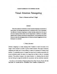
K (items) Figure 1. Distribution of the bootstrap estimates of (A) the processing capacity C, (B) t0 values, and (C) visual short term memory capacity of the left and the right visual fields in whole report.
MODELING VISUAL ATTENTION et al. (1999). In the whole report experiment, five target letters were shown in a column in either the left or the right visual field (3.3º from fixation). In the following, Stimulus Locations 1–5 denote the stimuli shown to the left, counting from top to bottom. Correspondingly, Stimulus Locations 6–10 denote the stimuli shown to the right, counting again from top to bottom. The exposure duration was varied between 70 and 200 msec. In half of the 12 conditions, the stimuli were unmasked, and in the remaining conditions, the letters were followed by pattern masks, in order to prevent further processing. A total of 15 parameters were estimated: Two t0 parameters at 18 msec (left) and 29 msec (right), 2 K parameters at 2.0 items (left) and 1.7 items (right), 1 μ parameter at 90 msec, and 10 different processing rates (v values) for each of the 10 display locations. The t0 values were limited by a minimum value of 0.0 sec, and the K values had a maximum of 2.0, the latter being due to a maximum observed score of two letters in the data set. The distribution of v values across the 10 display locations is shown in Table 3. The v values are clearly largest for the top locations, decreasing downward in the visual field on both the left and the right sides. Furthermore, processing capacity seems to be larger for the right than for the left visual field. To get an estimate of the total processing capacity within each hemifield, C values were calculated by summing the v values for each hemifield. This yielded two estimates of the processing capacity for each hemifield: CL ⫽ 6.5 letters/sec for the left and CR ⫽ 12.6 letters/sec for the right hemifield. The difference in processing capacity between the two hemifields was further explored using the bootstrap method with a total of 1,000 resamples. A plot of the distributions of the bootstrap estimates for the two processing capacities is shown in Figure 1A. There is little overlap of the two distributions, thus again suggesting that the processing capacity was larger in the right than in the left hemifield. A similar comparison was made for the t0 and K values between the two hemifields. The results of the bootstrap samples are shown in Figures 1B and 1C, respectively. There is no clear evidence for a systematic difference in either the t0 values or the K values.2 In the partial report experiment, the exposure duration was constant at 120 msec, and the stimulus letters were masked in all the conditions. The selection criterion was color: Letters were printed in either red or green and could appear at four possible display locations given by the corners of an imaginary square centered at fixation (5.0º ⫻ 5.0º). Within each block of 16 trials, either the red or the green letters were designated as targets, and the other set of letters as distractors. A total of 16 conditions were used: (1) 4 conditions with a single target, (2) 4 conditions with one target and one distractor in the same hemifield, (3) 4 conditions with one target and one distractor in opposite hemifields, (4) 2 conditions with two targets in the same hemifield, and (5) 2 conditions with two targets in opposite hemifields.
129
Table 4A Estimates of A Values in the Partial Report Experiment Top Bottom
Left 0.71 0.50
Right 1.86 0.79
A total of nine parameters were estimated fixing the VSTM capacity K at 2.0. Because only a single exposure duration was used in the partial report experiment, it was possible only to estimate A values, measuring the number of letters processed at each of the four possible stimulus locations. Similarly, an attentional weight was estimated for each of the four locations. The estimated A values and attentional weights are shown in Table 4A. The A values are lower in the left than in the right visual field and are lower for the lower than for the upper visual field. Given the results from the whole report experiment, this is most likely due to the difference in the C values. Note that the smallest A value is found for the bottom left position. Looking at the distribution of attentional weights for the targets in Table 4B, there seems to be a strong bias toward the two top display locations. Furthermore, the attentional weight of the lower left display location seems particularly low. The combined effect of low sensory uptake (low A value) and diminished attentional weights in the lower left quadrant of the visual field corresponds well with the patient’s tendency to neglect items in the lower left visual field when tested with the Mesulam cancellation task (Mesulam, 1985). Finally, a single α value was estimated to 0.35. A bootstrap analysis (1,000 resamples) showed moderately high variability of the α value (SD ⫽ 0.15; see Figure 2). Conclusions Bundesen’s (1990) theory of visual attention provides a unique framework for quantitative modeling of visual attention (see also Bundesen, 1998; Bundesen et al., 2005). However, implementing the TVA model to estimate parameters in relation to a specific experimental paradigm is both mathematically and technically challenging. Here, a new generalized mathematical framework is presented that extends previous derivations of the TVA (see Bundesen, 1990; Duncan et al., 1999; Shibuya & Bundesen, 1988). Furthermore, the generalized mathematical framework is implemented in a program package that provides a user friendly and flexible interface for both specifying a model to a particular whole or partial report paradigm and later fitting the model to a set of behavioral data. In future versions of the program package, we plan to include Table 4B Estimates of Attentional Weights of Targets in the Partial Report Experiment Top Bottom
Left 1.00 0.05
Right 0.73 0.14
130
KYLLINGSBÆK 180 160 140
Frequency
120 100 80 60 40 20 0 –0.2
0.0
0.2
0.4
0.6
0.8
1.0
1.2
α Figure 2. Distribution of the bootstrap estimates of the α value in partial report.
additional classic paradigms within the visual attention literature, such as visual search, Posner’s cued detection task (e.g., Posner, 1980), rapid serial visual presentation, and change detection. The program package has already been used successfully in a number of neuropsychological investigations (e.g., Duncan et al., 2003; Finke, Bublak, Dose, Müller, & Schneider, 2006; Habekost & Bundesen, 2003; Habekost & Rostrup, 2006; Hung, Driver, & Walsh, 2005; Peers et al., 2005). Moreover, a clinical version of the program package is under development, which will include norms from both healthy control subjects and different neurological and psychiatric patient populations (Bublak et al., 2005; Finke et al., 2005). REFERENCES Bishop, M. C. (2003). Neural networks for pattern recognition. Oxford: Oxford University Press. Broadbent, D. E. (1958). Perception and communication. Oxford: Oxford University Press. Broadbent, D. E. (1971). Decision and stress. London: Academic Press. Bublak, P., Finke, K., Krummenacher, J., Preger, R., Kyllingsbæk, S., Müller, H. J., & Schneider, W. X. (2005). Usability of a theory of visual attention (TVA) for parameter-based measurement of attention: II. Evidence from two patients with frontal or parietal damage. Journal of the International Neuropsychological Society, 11, 843-854. Bundesen, C. (1990). A theory of visual attention. Psychological Review, 97, 523-547. Bundesen, C. (1998). A computational theory of visual attention. Philosophical Transactions of the Royal Society of London: Series B, 353, 1271-1281. Bundesen, C., & Habekost, T. (2005). Attention. In K. Lamberts & R. Goldstone (Eds.), Handbook of cognition (pp. 105-129). London: Sage. Bundesen, C., Habekost, T., & Kyllingsbæk, S. (2005). A neural theory of visual attention: Bridging cognition and neurophysiology. Psychological Review, 112, 291-328. Bundesen, C., Kyllingsbæk, S., Houmann, K. J., & Jensen, R. M.
(1997). Is visual attention automatically attracted by one’s own name? Perception & Psychophysics, 59, 714-720. Bundesen, C., Kyllingsbæk, S., & Larsen, A. (2003). Independent encoding of colors and shapes from two stimuli. Psychonomic Bulletin & Review, 10, 474-479. Bundesen, C., Pedersen, L. F., & Larsen, A. (1984). Measuring efficiency of selection from briefly exposed visual displays: A model for partial report. Journal of Experimental Psychology: Human Perception & Performance, 10, 329-339. Bundesen, C., Shibuya, H., & Larsen, A. (1985). Visual selection from multielement displays: A model for partial report. In M. I. Posner & O. S. M. Marin (Eds.), Attention and performance XI (pp. 631649). Hillsdale, NJ: Erlbaum. Deutsch, J. A., & Deutsch, D. (1963). Attention: Some theoretical considerations. Psychological Review, 70, 80-90. Duncan, J. (1984). Selective attention and the organization of visual information. Journal of Experimental Psychology: General, 113, 501517. Duncan, J., Bundesen, C., Olson, A., Humphreys, G., Chavda, S., & Shibuya, H. (1999). Systematic analysis of deficits in visual attention. Journal of Experimental Psychology: General, 128, 450-478. Duncan, J., Bundesen, C., Olson, A., Humphreys, G., Ward, R., Kyllingsbæk, S., et al. (2003). Attentional functions in dorsal and ventral simultanagnosia. Cognitive Neuropsychology, 20, 675-701. Efron, B., & Tibshirani, R. J. (1993). An introduction to the bootstrap. New York: Chapman & Hall. Finke, F., Bublak, P., Dose, M., Müller, H. J., & Schneider, W. X. (2006). Parameter-based assessment of spatial and non-spatial attentional deficits in Huntington’s disease. Brain, 129, 1137-1151. Finke, F., Bublak, P., Krummenacher, J., Kyllingsbæk, S., Müller, H. J., & Schneider, W. X. (2005). Usability of a theory of visual attention (TVA) for parameter-based measurement of attention I: Evidence from normal subjects. Journal of the International Neuropsychological Society, 11, 832-842. Habekost, T., & Bundesen, C. (2003). Patient assessment based on a theory of visual attention (TVA): Subtle deficits after a right frontalsubcortical lesion. Neuropsychologia, 41, 1171-1188. Habekost, T., & Rostrup, E. (2006). Persisting asymmetries of vision after right side lesions. Neuropsychologia, 44, 876-895. Hung, J., Driver, J., & Walsh, V. (2005). Visual selection and posterior parietal cortex: Effects of repetitive transcranial magnetic stimulation on partial report analyzed by Bundesen’s theory of visual attention. Journal of Neuroscience, 25, 9602-9612.
MODELING VISUAL ATTENTION Logan, G. D. (1996). The CODE theory of visual attention: An integration of space-based and object-based attention. Psychological Review, 103, 603-649. Logan, G. D. (2002). An instance theory of attention and memory. Psychological Review, 109, 376-400. Logan, G. D., & Gordon, R. D. (2001). Executive control of visual attention in dual-task situations. Psychological Review, 108, 393-434. Luck, S. J., & Vogel, E. K. (1997). The capacity of visual working memory for features and conjunctions. Nature, 390, 279-281. Mesulam, M.-M. (Ed.) (1985). Principles of behavioral neurology: Tests of directed attention and memory. Philadelphia: Davis. Peers, P. V., Ludwig, C. J. H., Rorden, C., Cusack, R., Bonfiglioli, C., Bundesen, C., et al. (2005). Attentional functions of parietal and frontal cortex. Cerebral Cortex, 15, 1469-1484. Posner, M. I. (1980). Orienting of attention: The VII Sir Frederic Bartlett Lecture. Quarterly Journal of Experimental Psychology, 32, 3-25. Press, W. H., Teukolsky, S. A., Vetterling, W. T., & Flannery, B. P. (2002). Numerical recipes in C⫹⫹. Cambridge: Cambridge University Press.
Ross, S. M. (2000). Introduction to probability and statistics for engineers and scientists. San Diego: Academic Press. Shibuya, H., & Bundesen, C. (1988). Visual selection from multielement displays: Measuring and modeling effects of exposure duration. Journal of Experimental Psychology: Human Perception & Performance, 14, 591-600. Siegel, S., & Castellan, N. J., Jr. (1988). Nonparametric statistics for the behavioral sciences (2nd ed.). New York: McGraw-Hill. Sperling, G. (1960). The information available in brief visual presentations. Psychological Monographs: General & Applied, 74, 1-29. Wheeler, M. E., & Treisman, A. M. (2002). Binding in short-term visual memory. Journal of Experimental Psychology: General, 131, 48-64. NOTES 1. The program package, including manual and exemplary data sets, is available for free download on the Internet at www.psy.ku.dk/cvc/. 2. The sharp peaks seen in the bootstrap distributions of t0 (at 0.0; see Figure 1B) and K (at 2.0; see Figure 1C) are due to the limits imposed on the parameter estimates.
APPENDIX Equations 5 and 6 define the probability of reporting a given set of stimuli R when a set of stimuli S is presented in whole report. Given the density and distribution probability function in Equations 3 and 4, closed-form formulas will be derived in the following. These formulas are implemented as algorithms in the WinTVAFit program described in the present article. The derivation from Equation 5 simply follows by insertion of the distribution function from Equation 4: If n(R) ⬍ K or n(R) ⫽ K ⫽ n(S), then Ps ( R ) = = =
∏ Fi (τ ) ∏
i ∈R
j ∈S − R
1 − Fj (τ )
∏ ⎡⎣1 − exp ( − viτ )⎤⎦ ∏
i ∈R
j ∈S − R
(
exp − v j τ
)
⎛
⎞ vj $ τ ⎟ , ⎝ j ∈S − R ⎠
∏ ⎡⎣1 − exp ( − viτ )⎤⎦ exp ⎜ − ∑
i ∈R
(A1)
where n(R) and n(S) are the number of items in R and S, respectively, K is the capacity of VSTM, and τ is the effective exposure duration equal to t ⫺ t0. For Equation 6, matters are more complicated: If n(R) ⫽ K ⬍ n(S), then PS ( R ) = = = = =
τ
∑ ∫ f i (t ) ∏
i ∈R 0
j ∈R −{i}
F j (t )
∏
k ∈S − R
τ
∑ ∫ vi exp ( − vit ) ∏
i ∈R 0
j ∈R −{i}
τ
∑ vi ∫ exp ( − vit )
i ∈R
0
τ
i ∈R
∑ vi
i ∈R
1 − Fk (t ) dt
(
∑
∏
k ∈S − R
exp ( − vk t ) dt
⎛ ⎞ ⎛ ⎞ ( −1)n( J ) exp ⎜ − ∑ v j t ⎟ exp ⎜ − ∑ vk t ⎟ dt ⎝ ⎠ ⎝ ⎠ J ∈P ( R −{i}) j ∈J k ∈S − R
∑
∑
J ∈P ( R −{i})
)
⎡1 − exp − v j t ⎤ ⎣ ⎦
⎡ ⎛ ( −1)n( J ) exp ⎢ − ⎜ vi + 0 J ∈P ( R −{i}) ⎣ ⎝
∑ vi ∫
⎛ ( −1)n( J ) G ⎜ vi + ⎝
j ∈J
∑ vj + ∑
j ∈J
⎞ ⎤ vk ⎟ t ⎥ dt k ∈S − R ⎠ ⎦
∑ vj + ∑ k ∈S − R
⎞ vk ⎟ , ⎠
(A2)
where 1 − exp( − v τ ) . v In line 3 of Equation A2, P(R ⫺ {i}) stands for the power set of the set R ⫺ {i}. By the power set P(A) is meant the set of all subsets of A. That is, if A ⫽ {a,b,c}, P(A) ⫽ { {Ø}, {a}, {b}, {c}, {a,b}, {a,c}, {b,c}, {a,b,c} }. Thus, the expression J ∈ P(R ⫺ {i}) means that J runs through all the possible subsets of R ⫺ {i}. The use of the power set is an extension of Newton’s binomial expansion, which transforms a series of products into a sum. G(v ) =
131
132
KYLLINGSBÆK APPENDIX (Continued) Formulas for partial report similar to Equations A1 and A2 can also be derived. First, however, it is necessary to define P′(A,i), the class of all subsets of A that have a cardinal number equal to i. If, for example, A ⫽ {a,b,c}, then P′(A,2) ⫽ { {a,b}, {a,c}, {b,c} }. Furthermore, let ST and SD be the set of presented targets and distractors, respectively, and let S ⫽ ST ∪ SD. Correspondingly, let RT be the set of targets reported, and let RD be the set of distractors that enter VSTM but are not reported. According to TVA, distractors may enter VSTM along with targets, but the distractors are not reported by the participant. Consider the probability PS(RT) that the set of sampled targets (the report), given that S is displayed, equals RT , where 0 ⱕ n(RT) ⱕ K. PS(RT) may be defined as a sum of three probabilities, P1 , P2 , and P3—that is, PS ( RT ) = P1 + P2 + P3 . P1 is the probability that the report equals RT and VSTM is not filled up (i.e., n(RT) ⫹ n(RD) ⬍ K). If n(RT) ⫽ K, P1 is zero; otherwise, P1 =
∏ Fi (τ ) ∏
i ∈RT
j ∈ST − RT
K − n( RT ) −1
∑
$ =
∑
∏ Fl (τ ) ∏
J ∈P ′( SD ,k ) l ∈J
k =0
m ∈SD − J
∏ ⎡⎣1 − exp ( − viτ )⎤⎦ ∏
i ∈RT
j ∈ST − RT
K − n( RT ) −1
∑
$ =
1 − F j (τ ) 1 − Fm (τ )
(
exp − v jτ
)
∏ ⎣⎡1 − exp ( − ulτ )⎤⎦ ∏
∑
J ∈P ′( SD ,k ) l ∈J
k =0
m ∈SD − J
exp ( − umτ )
⎛
⎞ v jτ ⎟ ⎝ j ∈ST − RT ⎠
∏ ⎡⎣1 − exp ( − viτ )⎤⎦ exp ⎜ − ∑
i ∈RT
K − n( RT ) −1
∑
$
⎛
⎞ umτ ⎟ , ⎝ m ∈SD − J ⎠
∏ ⎡⎣1 − exp ( − ulτ )⎤⎦ exp ⎜ − ∑
∑
J ∈P ′( SD ,k ) l ∈J
k =0
(A3)
where the terms with i as the running variable represent the set of targets finishing processing before τ, the terms with j represent the set of targets that do not finish processing, the terms with l represent distractors finishing processing, and finally the terms with m represent distractors that do not finish processing before τ. Note also that the processing rates of distractors are represented by u, rather than v, values in order to make it easier to distinguish rates of targets and rates of distractors in the equations. P2 is the probability that the report equals RT, the VSTM is filled up (i.e., n(RT) ⫹ n(RD) ⫽ K), and the last item to enter VSTM is a target. If n(RT) ⫽ 0 or n(RT) ⬍ K ⫺ n(SD), P2 is zero; otherwise, P2 =
τ
∑ ∫ f i (t ) ∏
i ∈RT 0
j ∈RT −{i}
∑
$
F j (t )
∏
k ∈ST − RT
∏ Fl (t ) ∏
J ∈P ′( SD , K − n( RT )) l ∈J
=
m ∈SD − J
τ
∑ ∫ vi exp ( − vit ) ∏
i ∈RT 0
j ∈RT −{i}
1 − Fm (t ) dt
J ∈P ′( SD , K − n( RT )) l ∈J
=
τ
∑ ∫ vi expp ( − vit )
i ∈RT 0
$
∑
τ
∑ vi ∫
i ∈RT
⎛ ⎞ ( −1)n( L ) exp ⎜ − ∑ v j t ⎟ ⎝ j ∈L ⎠ L ∈P( RT −{i})
∑
∑ vj + ∑
j ∈L
∏
k ∈ST − RT
exp ( − vk t )
⎛ ⎞ ( −1)n( M ) exp ⎜ − ∑ ul t ⎟ ∏ exp ( − umt ) dt ⎝ l ∈M ⎠ m ∈SD − J
∑
0 L ∈P( RT −{i}) J ∈P ′( SD , K − n( RT )) M ∈P ( J )
⎡ ⎛ $ exp ⎢ − ⎜ vi + ⎢⎣ ⎝
exp ( − vk t )
exp ( − umt ) dt
∑
∑
∑
∏
k ∈ST − RT
m ∈SD − J
J ∈P ′( SD , K − n( RT )) M ∈P ( J )
=
)
(
⎡1 − exp − v j t ⎤ ⎣ ⎦
∏ ⎡⎣1 − exp ( − ul t )⎤⎦ ∏
∑
$
1 − Fk (t )
k ∈ST − RT
vk +
( −1)n( L ) + n( M ) ⎞ ⎤ um ⎟ t ⎥ dt ⎠ ⎥⎦ m ∈SD − J
∑ ul + ∑
l ∈M
MODELING VISUAL ATTENTION APPENDIX (Continued) =
∑ vi
∑
∑
⎛ $ G ⎜ vi + ⎝
∑ vj + ∑
i ∈RT
∑
L ∈P( RT −{i}) J ∈P ′( SD , K − n( RT )) M ∈P ( J )
j ∈L
k ∈ST − RT
vk +
( −1)n( L ) + n( M ) ⎞ um ⎟ , ⎠ m ∈SD − J
∑ ul + ∑
l ∈M
(A4)
where element i is the last of the targets to enter VSTM, j runs across the set of the targets that entered before target i, k represents the targets that do not finish processing before VSTM is filled up, l represents the distractors that enter VSTM before target i, and finally m represents the distractors that do not finish processing before VSTM is filled up. Finally, P3 is the probability that the report equals RT, the VSTM is filled up (i.e., n(RT) ⫹ n(RD) ⫽ K), and the last item to enter VSTM is a distractor. If n(RT) ⫽ K or n(RT) ⬍ K ⫺ n(SD), P3 is zero; otherwise, P3 =
τ
∑ ∫ f i (t ) ∏
i ∈SD 0
j ∈RT
F j (t )
∑
$
∏
k ∈ST − RT
1 − Fk (t )
∏ Fl (t )
J ∈P ′( SD −{i}, K − n( RT ) −1) l ∈J
=
τ
∏
m ∈SD −{i}− J
(
)
∑ ∫ ui exp ( − uit ) ∏
⎡1 − exp − v j t ⎤ ⎣ ⎦
∑
∏ ⎡⎣1 − exp ( − ul t )⎤⎦
i ∈SD 0
j ∈RT
$
∏
k ∈ST − RT
J ∈P ′( SD −{i}, K − n( RT ) −1) l ∈J
=
1 − Fm (t ) dt
τ
exp ( − vk t )
∏
m ∈SD −{i}− J
exp ( − umt ) dt
⎛ ⎞ ( −1)n( L ) exp ⎜ − ∑ v j t ⎟ ∏ exp ( − vk t ) ⎝ ⎠ k ∈ST − RT j ∈L L ∈P( RT )
∑ ∫ ui exp ( − uit ) ∑
i ∈SD 0
⎛ ⎞ ( −1)n( M ) exp ⎜ − ∑ ul t ⎟ ∏ exp ( − umt ) dt ⎝ ⎠ m ∈SD −{i}− J l ∈M J ∈P ′( SD −{i}, K − n( RT ) −1) M ∈P ( J )
∑
$ =
=
∑
τ
∑ ui ∫ ∑
∑
⎡ ⎛ $exp ⎢ − ⎜ ui + ⎢⎣ ⎝
∑ vj + ∑
∑
i ∈SD
∑
0 L ∈P( RT ) J ∈P ′( SD −{i}, K − n( RT ) −1) M ∈P ( J )
i ∈SD
ui
∑
j ∈L
k ∈ST − RT
vk +
∑
∑ ul +
l ∈M
∑
L ∈P( RT ) J ∈P ′( SD −{i}, K − n( RT ) −1) M ∈P ( J )
⎛ $ G ⎜ ui + ⎝
∑ vj + ∑
j ∈L
k ∈ST − RT
vk +
∑ ul +
l ∈M
( −1)n( L ) + n( M ) ⎞ ⎤ um ⎟ t ⎥ dt ⎠ ⎥⎦ m ∈SD −{i}− J
∑
( −1)n( L ) + n( M )
⎞ um ⎟ , ⎠ m ∈SD −{i}− J
∑
where item i is the last distractor to enter VSTM. (Manuscript received November 1, 2004; accepted for publication March 7, 2005.)
(A5)
133