Jan 18, 2006 ... Department of Chemical Engineering. İzmir Institute of ... neural networks and
encouragement through my hardest times. I would like to express ...
MODELLING AND CONTROL OF BIOPROCESSES BY USING ARTIFICIAL NEURAL NETWORKS AND HYBRID MODEL
A Thesis Submitted to the Graduate School of Engineering and Science of zmir Institute of Technology in Partial Fulfillment of the Requirements for the Degree of MASTER OF SCIENCE in Chemical Engineering
by Ömer Sinan GENÇ
January 2006 ZM R
We approve the thesis of Ömer Sinan GENÇ
Date of Signature
………………………………………… Asst. Prof. Dr. Ay egül BATIGÜN Supervisor Department of Chemical Engineering zmir Institute of Technology
18 January 2006
………………………………………… Asst. Prof. Dr. O uz BAYRAKTAR Department of Chemical Engineering zmir Institute of Technology
18 January 2006
…………………………………………. Asst. Prof. Dr. Serhan ÖZDEM R Department of Mechanical Engineering zmir Institute of Technology
18 January 2006
………………………………………… Prof. Dr. Devrim BALKÖSE Head of Department zmir Institute of Technology
18 January 2006
................................................... Assoc. Prof. Dr. Semahat ÖZDEM R Head of the Graduate School
ii
ACKNOWLEDGEMENTS
I would like to express my sincere gratitude to my advisors Asst. Prof. Ay egül Batigün for her supervision, support, and confidence during my studies. I would like to thank to Asst. Prof. O uz Bayraktar for him help and encouragement. And special thanks to Asst. Prof. Serhan Özdemir for him valuable recommendations on artificial neural networks and encouragement through my hardest times. I would like to express my gratitude to my family, for their loving care and efforts. I especially like to thank my parents, for sharing my stress and emotions, and for the respect they showed to me. Finally, I am also grateful to my friends for their friendship and for sharing their ideas about many issues, giving me the inspiration to complete this work.
ABSTRACT
The aim of this study is modeling and control of bioprocesses by using neural networks and hybrid model techniques. To investigate the modeling techniques, ethanol fermentation with Saccharomyces Cerevisiae and recombinant Zymomonas mobilis and finally gluconic acid fermentation with Pseudomonas ovalis processes are chosen. Model equations of these applications are obtained from literature. Numeric solutions are done in Matlab by using ODE solver. For neural network modeling a part of the numerical data is used for training of the network. In hybrid modeling technique, model equations which are obtained from literature are first linearized then to constitute the hybrid model linearized solution results are subtracted from numerical results and obtained values are taken as nonlinear part of the process. This nonlinear part is then solved by neural networks and the results of the neural networks are summed with the linearized solution results. This summation results constitute the hybrid model of the process. Hybrid and neural network models are compared. In some of the applications hybrid model gives slightly better results than the neural network model. But in all of the applications, required training time is much more less for hybrid model techniques. Also, it is observed that hybrid model obeys the physical constraints but neural network model solutions sometimes give meaningless outputs. In control application, a method is demonstrated for optimization of a bioprocess by using hybrid model with neural network structure. To demonstrate the optimization technique, a well known fermentation process is chosen from the literature.
iv
ÖZET
Bu çalı manın amacı biyoproseslerin yapay sinir a ları ve hibrit model teknikleri ile modellenmesi ve kontrolüdür. Modeleme tekniklerinin incelenmesi için ethanolün Saccharomyces Cerevisiae ve Zymomonas mobilis organizmaları ile glukonik asidin Pseudomonas ovalis organizması ile fermentasyonunu içeren prosesler seçilmi tir. Seçilen bu proseslerin model denklemleri literatürden elde edilmi ve bu denklemlerin nümerik cözümleri Matlab’in ODE fonksiyonu kullanılarak hesaplanm tır. Nümerik sonuçların bir kısmı yapay sinir a larının ö renme kısmında kullanılmı tır. Hibrit modelleme tekni inde, literatürden elde edilen model denklemler lineer hale getirilmi ve hidrit modeli olu turmak için bu lineer denklemlerin çözümleri nümerik sonuçlardan çıkarılmı tır. Elde edilen bu sonuçlar sistemin lineer olmayan kısmı olarak ele alınmı ve bu kısım yapay sinir a ları ile modellenmi tir. Sinir a ları kullanılarak elde edilen bu sonuçlar lineer sonuçlarla birle tirilmi ve prosesin hibrit modeli elde edilmi tir. Daha sonra hibrit model sonuçları ve sinir a ları ile yapılan modellemenin sonuçları kar ıla tırılmı tır. Bazı uygulamalarda hibrit model, yapay sinir a
modeline kıyasla daha
iyi sonuçlar vermi tir. Ancak bütün uygulamalarda
görülmü tür ki, hibrit model için gerekli olan ö renme zamanı tüm sistemin sinir a ı ile modellenmesi için gerekli olandan çok daha azdır. Ayrıca, hibrit modelin fiziksel ko ullara uygun davrandı ı öte yandan da yapay sinir a modellerin bazen anlamsız sonuçlar verdi i görülmü tür. Kontrol uygulamaları kısmında, bioproseslerin optimizasyonu gerçekle tirmek üzere kullanılacak bir hibrit model algoritması geli tirilmi tir. Bu optimizasyon algoritmasının gösterilmesi için bir fermentasyon prosesi seçilmi
ve modelin
uygulanma ekli anlatılmı tır.
v
TABLE OF CONTENTS
LIST OF FIGURES ....................................................................................................... viii LIST OF TABLES........................................................................................................... xi CHAPTER 1. INTRODUCTION ................................................................................... 1 CHAPTER 2. NEURAL NETWORKS .......................................................................... 3 2.1 General Information on Neural Networks ............................................. 3 2.1.1 Neural Networks .............................................................................. 3 2.1.2 Training Algorithm .......................................................................... 4 2.1.3 Structure of Neural Networks .......................................................... 5 2.1.4 The Usage of Neural Networks in Bioprocesses ............................. 7 2.2 General Information on Grey-Box Mode ............................................. l8 2.2.2 Types of Hybrid Models .................................................................. 8 2.2.3 The Usage of Hybrid Models ......................................................... 10 CHAPTER 3. PROCESS CONTROL BY ANN AND HYBRID MODEL................. 13 3.1 Batch Process Control.......................................................................... 13 3.2 ANN’s In Process Control ................................................................... 14 CHAPTER 4. BIOPROCESSES AND BIOREACTORS ............................................ 19 4.1 What Is Bioprocess And Biotechnology? ............................................ 19 4.2 General Information on Bioprocesses.................................................. 19 4.2.1 Compartmental Models .................................................................. 20 4.2.2 Metabolic Models........................................................................... 21 4.2.3 Growth Kinetics ............................................................................. 21 4.3 Bioreactors ........................................................................................... 23 4.3.1 Rate Laws....................................................................................... 24 4.3.2 Stoichiometry ................................................................................. 25 vi
4.3.3 Substrate Accounting ..................................................................... 26 4.3.4 Mass Balances ................................................................................ 26 4.3.5 Design Equations............................................................................ 27 CHAPTER 5. PROPOSED WORK.............................................................................. 29 CHAPTER 6. APPLICATION OF
NEURAL AND HYBRID MODELS
ON BIOPROCESSES.......................................................................... 32 6.1 Case Study 1: Ethanol fermentation with Saccharomyces Cerevisiae ............................................................................................ 32 6.2 Case Study 2: Ethanol production with recombinant Zymomonas mobilis ............................................................................. 46 6.3 Case Study 3: Gluconic acid fermentation with organism Pseudomonas ovalis............................................................................ 61 CHAPTER 7. CONTROL STUDY .............................................................................. 76 7.1 Control Implications ............................................................................ 76 CHAPTER 8. CONCLUSION...................................................................................... 81 REFERENCES ............................................................................................................... 83 APPENDICES APPENDIX A. CONSTANTS OF CASE STUDY 1..................................................... 86 APPENDIX B. CONSTANTS OF CASE STUDY 2..................................................... 88 APPNEDIC C. CONSTANTS OF CASE STUDY 3 ..................................................... 92
vii
LIST OF FIGURES
Figure
Page
Figure 2.1. A single neuron, receiving a weighted summation from neurons in a previous layer........................................................................................ 4 Figure 2.2. A feed forward artificial neural network configuration............................... 6 Figure 2.3. Hybrid model Scheme ................................................................................. 9 Figure 2.4. Parallel structure of grey-box model with neural network ........................ 10 Figure 2.5. Serial structure of a grey box model with neural network......................... 10 Figure 2.6. ANN and Hybrid model predictions of process behavior.......................... 11 Figure 2.7. Comparison between hybrid model and neural network model predictions(dimensionless values) ............................................................. 12 Figure 3.1. Neural networks in general model predictive control strategy .................. 14 Figure 3.2. On-line control implementation of neural network for controlling the cell concentration along the profile x=0.2×time when the network was trained for a profile of x=0.15×time. • Experimental value; _ prediction with online adaptation of weights; prediction without adaptation of weights.................................................................... 15 Figure 3.3. Hybrid model structure for the fermentation process ................................ 16 Figure 3.4
Proposed control system’s block diagram ................................................. 17
Figure 3.5. Performance of adaptive neural PID control-deterministic case ............... 17 Figure 4.1. Time versus log cell concentration graph of growth mechanism ............ 22 Figure 5.6. Schematic view of Neural Network model................................................ 30 Figure 5.7. Schematic view of Hybrid Model.............................................................. 31 Figure 6.1. Linearized and exact solution of cell concentration vs. time..................... 38 Figure 6.2. Linearized and exact solution of glucose concentration vs. time .............. 39 Figure 6.3. Linearized and exact solution of product concentration vs. time .............. 39 Figure 6.4. Neural network and exact solution of cell concentration vs. time............. 40
viii
Figure 6.5. Neural network and exact solution of glucose concentration vs. time ............................................................................................................ 41 Figure 6.6. Neural network and exact solution of product concentration vs. time ............................................................................................................ 42 Figure 6.7. Hybrid, linearized and exact solution of cell concentration vs. time ............................................................................................................ 43 Figure 6.8. Hybrid, linearized and exact solution of glucose concentration vs. time....................................................................................................... 44 Figure 6.9. Hybrid, linearized and exact solution of product concentration vs. time....................................................................................................... 45 Figure 6.10. Exact and linearized solutions of biomass vs. time ................................... 50 Figure 6.11. Exact and linearized solutions of glucose uptake vs. time ........................ 51 Figure 6.12. Exact and linearized solutions of xylose uptake vs. time .......................... 52 Figure 6.13. Exact and linearized solutions of ethanol production vs. time .................. 53 Figure 6.14. Neural network solution of biomass vs. time ............................................ 54 Figure 6.15. Neural network solution of glucose uptake vs. time.................................. 55 Figure 6.16. Neural network solution of xylose uptake vs. time ................................... 56 Figure 6.17. Neural network solution of ethanol production (product) vs. time............ 56 Figure 6.18. Hybrid model solution of biomass vs. time ............................................... 57 Figure 6.19. Hybrid model solution of glucose uptake vs. time .................................... 58 Figure 6.20. Hybrid model solution of xylose uptake vs. time ...................................... 59 Figure 6.21. Hybrid model solution of ethanol production (product) vs. time .............. 60 Figure 6.22. Linearized and exact solution of cell concentration vs. time..................... 64 Figure 5.23. Linearized and exact solution of gluconic acid concentration vs. time ............................................................................................................ 64 Figure 6.24. Linearized and exact solution of gluconolactone concentration vs. time....................................................................................................... 65 Figure 6.25. Linearized and exact solution of glucose concentration vs. time .............. 66 Figure 6.26. Linearized and exact solution dissolved oxygen concentration vs time ............................................................................................................ 66 Figure 6.27. Neural network and exact solution cell concentration vs. time ................. 67 Figure 6.28. Neural network and exact solution gluconic acid concentration vs. time....................................................................................................... 68
ix
Figure 6.29. Neural network and exact solution gluconolactone concentration vs. time....................................................................................................... 69 Figure 6.30. Neural network and exact solution Glucose concentration vs. time ............................................................................................................ 70 Figure 6.31. Neural
network
and
exact
solution
dissolved
oxygen
concentration vs. time ................................................................................ 71 Figure 6.32. Hybrid, linearized and exact solution of cell concentration vs. time ............................................................................................................ 72 Figure 6.33. Hybrid, linearized and exact solution of gluconic acid concentration vs time ................................................................................. 73 Figure 6.34. Hybrid, linearized and exact solution of gluconolactone concentration vs. time ................................................................................ 74 Figure 6.35: Hybrid, linearized and exact solution of glucose concentration vs. time....................................................................................................... 74 Figure 6.36. Hybrid, linearized and exact solution of dissolved oxygen concentration vs. time ................................................................................ 75 Figure 7.1. Schematic view of steps in control implication ......................................... 80
x
LIST OF TABLES
Table
Page
Table 6.1.
Additional data for process ........................................................................ 33
Table 6.2.
Initial values for the batch fermentation with =0.65................................ 47
Table 6.3.
Optimal kinetic parameters for biomass production model (all data sets with =0.65) ................................................................................ 47
Table 6.4.
Optimal kinetic parameters for glucose/xylose consumption model (all data sets with =0.65)............................................................... 48
Table 6.5.
Optimal kinetic parameters for ethanol production (all data sets with =0.65)............................................................................................... 48
Table 6.6.
Parameters used in the modeling of gluconic acid production .................. 62
xi
CHAPTER 1 INTRODUCTION Strongly nonlinear behavior found in chemical engineering and bio-engineering processes such as highly exothermic reactors and pH processes. On the other hand, chemical and bio processes are time variant because of their nature. This characteristic property makes them hard to control. To control these processes by using the conventional methods is time-consuming and very expensive. As it is known there are lots of parameters and variables in chemical and bioprocesses. For modeling and controlling these processes all of the dependencies and changes in the parameters and variables should be known. Obtaining this dependencies and changes can not be easy every time and in some situations it is impossible. Thus, modeling and controlling of such processes is very difficult. At this point artificial neural networks attract the attention. Especially in past two decades, they are widely used in many fields of science and engineering. They are one of the fastest growing areas of artificial intelligence. Neural networks are the computers programs that simulate the learning process of human brain. As known human brain learns from the past experience and this situation is same for the neural networks. There are several types of network structure and training algorithms. As mentioned above, neural networks learn from the experience means that for using neural networks data are needed. These data are obtained from the past experiments or inputoutput values of the processes. There is lots of modeling and control studies in the literature (Wang et al., 1998, Ramirez and Jackson, 1999, Zorzetto et al., 2000, Molga, 2003, Olivera 2004) and these studies show us the efficiency of neural networks. But in some situations neural networks fails. Sometimes meaningless outputs are obtained. The reason is, in using neural networks, knowledge about the processes is not needed. The results are obtained from the past experiences. To avoid these kinds of situations, grey-box modeling can be used. In hybrid model structure the known parts of the process is modeled by mechanistic model and neural networks used for modeling the unknown parts of the processes. By this way more correct and more accurate results can be obtained. 1
The aim of this study is modeling and control of bioprocesses by using artificial neural networks and hybrid structure. In modeling with artificial neural network, data which are obtained from the processes are used in neural network training section and according to these trained networks process is modeled. In hybrid structure section, the linearized model is obtained and the results will be checked with the nonlinear model. After that, the nonlinear part of the process is solved by neural networks and finally the results are compared.
2
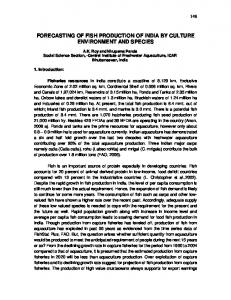
CHAPTER 2 NEURAL NETWORKS 2.1 General Information on Neural Networks 2.1.1 Neural Networks Neural Networks are the computer programs that simulate the learning process of the human brain. Like brain, the network structure composed of several processing elements called as neurons or nodes. These neurons which are located in the structure are highly interconnected with each other according to the type of the neural network. Connections can be done in several ways. Training algorithm and the structure of the network, changes with the changing of connection types. The first artificial neuron was produced in 1943 by the neurophysiologist Warren McCulloch and the logician Walter Pits. But the technology available at that time did not allow them to do too much. An artificial neuron consists of six main part and these are, inputs, bias, synaptic weights, net information, activation functions and outputs. It may have several inputs but it has got only one output. The neuron has two modes of operation; the training mode and the using mode. In the training mode the neurons are used for training algorithm and adjusting the weights. When the weights are adjusted then it can be used in the using mode. Here the weights are the values of the connection links. Bias node is generally used to account for the uncertainty effects. In the system there may be some parameters that affects the process but not considered. So by the bias node these effects are taken into consideration. Schematic view of typical neuron is shown in Figure 2.1.
3
Figure 2.1. A single neuron, receiving a weighted summation from neurons in a previous layer. (Source: Aguiar and Filho 2001) Many functions can be used as a transfer function in the neurons but especially in feed forward structure the most chosen ones are sigmoid, pure line and hyperbolic tangent function.
2.1.2 Training Algorithm There are two major types of training algorithms. These are supervised training and unsupervised training. In supervised training, both the inputs and the outputs are provided. The network then processes the inputs and compares its resulting outputs against the desired outputs. Errors are then propagated back through the system, causing the system to adjust the weights which control the network. This process occurs over and over as the weights are continually tweaked. The set of data which enables the training is called the "training set" If there is not enough training data, the network cannot be learn and so it cannot converge to the desired outputs. On the other hand, if there is enough data and again the network cannot converge then the input -output patterns and the structure of the network should be reviewed. By changing the number of hidden layers and changing the transfer functions network can converge. Also here, the training algorithms gain importance. As it mentioned, generally a feed forward algorithm can converge any nonlinear function. By changing the transfer functions, number of layers and the training algorithms, time necessary for convergence can be decreased. When desired outputs are obtained, the weights are frozen and networks 4
become ready for simulation. The other type of training is called unsupervised training. In unsupervised training, the network is provided with inputs but not with desired outputs. The system itself must then decide what features it will use to group the input data. This is often referred to as self-organization or adaption. At the present time, unsupervised learning is not well understood. This adaptation to the environment is the promise which would enable science fiction types of robots to continually learn on their own as they encounter new situations and new environments. Life is filled with situations where exact training sets do not exist. Some of these situations involve military action where new combat techniques and new weapons might be encountered. Especially in supervised training the most chosen training algorithm is feed forward back propagation.
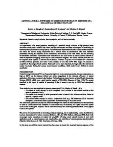
2.1.3 Structure of Neural Networks There are several types of neural networks such as, feed forward back propagation, recurrent neural networks, Cascade Correlation Neural networks and Radial basis neural networks. The most chosen one is the feed forward back propagation neural networks. In these types of structure there must be at least one input, one hidden and one output layer. The first layer called as input layer and the last layer called as output layer. The layers between the input and output layer is called as hidden layers. The number of the hidden layer can be change according to the nonlinearity of the process. Each process variable value is given to the one neuron in the input layer. In feed forward back propagation type nets information is always transmitted forward from each node in a layer to all nodes in the following layer. Each process variable value is given to one node in the input layer. The neurons on the first hidden layer receive a weighted summation of signals from input nodes, added to the bias term. The weights are specific for each connection and the bias terms are specific for each receiving node, allowing each node to receive a distinct value. The summed values are altered by a transfer function, which transforms the signal to a value. The transformed value will be the output of the node and will be transmitted to the next layer in the same manner and from one layer to the other layer until the output layer releases the net output. A schematic view of feed forward artificial neural network is shown in Figure 2.2.
5
Figure 2.2. A feed forward artificial neural network configuration (Source: Karım et al. 1997) In detail, back propagation algorithm can be divided into two passes, forward and backward pass. In the forward pass, flow direction of the information is from input layer to hidden layer and hidden layer to the output layer. In this pass, pairs are selected and fed into the input neurons after that these fed inputs are multiplied by the weights and then summed to form net information. The obtained net information is then squashed by the activation function and produce output. These produced outputs are then passed each neuron in the successive layer and finally at the end net output is obtained from the output neuron. Up to now, the forward pass is completed then backward pass starts. Here the transmission flow direction is form output layer to hidden layer and hidden layer to the input layer. Obtained outputs are checked with the desired ones and then errors are calculated. According to these errors all of the weights are adjusted generally by using the generalized delta rule. Here the connection weights are calculated as follows;
Wij
new
= Wij
old
+µ×
∂E (Wij ) ∂Wij
(2.1)
where W, µ and E represents weight, learning rate and error respectively. Errors can be calculated as; 6
1 E= 2
p
q
i =1 j =1
( y j − ti ) 2
(2.2)
and here p is the number of training patterns, q is the number of output nodes, ti and y represents the target output and model output respectively.
2.1.4 The Usage of Neural Networks in Bioprocesses Chemical and bioprocesses are strongly nonlinear processes, and because of their nature they are time variant. Thus, biological processes can be called as nondeterministic systems. The models of such processes are very complex and on the other hand modeling these processes is very difficult. There are lots of parameters change dependently or independently such as, microbiological growth rate and reaction kinetics. Also there are several parameters that cannot be measured directly from the systems and because of these uncertain parameters models could not describe the systems exactly. Thus on-line monitoring and controlling of such processes become nearly impossible. To overcome this situation, neural networks and some other computer programs are used. Neural networks have ability to learn from experience (collected data) instead of deep theoretical knowledge and networks can recognize the cause effect relationships ,furthermore they can filter the noise in the system and all these features makes them different from the other programs. In the literature there are several studies with neural networks on bioprocesses. Ramirez and Jackson (1999) used neural networks in modeling and controlling of erythromycin acetate salts pH and they conducted at the facilities of Abbott Chemical Plant with the purpose of studying the disturbance and compensation effects in the extraction process. Then they determine the time delay between the perturbation variable and the pH. Karım et al.(1997) studied on microbiological systems and they report that neural networks are suitable for modeling biological systems and emphasize the importance of the training data selection. As a case study they deal with Z.mobilis fermentation producing ethanol. They used neural network as state estimator. Aguiar and Filho (2001) investigated the modeling techniques to predict the pulping degree in paper industry and obtained mill values in desired accuracy and modeled the system. Nascimento et al. (2000) study on 7
optimization of nylon 6-6 polymerization in a twin extruder reactor and acetic anhydride plant. As a result they obtained % 20-30 increase in the polymer production with choosing the better operation conditions, on the other hand, in acetic anhydride plant they decrease the residual gas and natural gas on the raw anhydride process. Like these, there are several studies can be found in literature about modeling and control of fermentation and other biotechnological processes. The common points of all these studies is, in all the researchers consume less time in modeling the system and obtained successful results.
2.2 General Information on Grey-box model 2.2.1 Definition of Hybrid Model Hybrid model is a computational structure consisting of a neural network of computational nodes, which represents process knowledge at different levels of sophistication. In hybrid structure the known parts of the process are modeled by the mechanistic model known as the first principle model. The unknown parts of the system are modeled by neural networks. Thus, the network structure becomes smaller so the consumed time in adaptation will be smaller. On the other hand, obtaining meaningless outputs will be prevented by modeling the system with hybrid structure. But in this case, the controller must have knowledge about the process. As mentioned above in modeling the process with ANN the controller knowledge is not required. In chemical and bioprocesses there are several parameters which are changing with time or with the interaction of variables in the process. Also obtaining the values of these parameters can not easy or possible in every process. Thus, they become unknown parameters in the system. So that these parameters are modeled by neural networks and then combined with the mechanistic model.
2.2.2 Types of Hybrid Models The choice of how to combine both parts depends on the amount of knowledge about the process and quality and quantity of the available data. General view of hybrid
8
structure is shown in Figure 2.3 (Aguiar, Filho 2001). Especially, there are two types of connection and hybrid model; Parallel and Serial type of hybrid models.
Figure 2.3. Hybrid model Scheme, (Source: Aguiar H. and Filho R. 2001) In parallel structure, can be seen in Figure 2.4 (Xiong , Jutan 2002), the output of the grey-box model is the sum of two separate model outputs which are the outputs of approximate model and outputs of neural network. The neural network is placed in parallel and captures both model mismatch and process disturbances. In this architecture the load on the neural network is much lower when compared with a black box neural model which tries to model the entire process. This occurs because the approximate model captures most of the main process dynamics and leaving the remainder for the neural network. Thus, the size of the neural network can be substantially reduced.
9
Figure 2.4. Parallel structure of grey-box model with neural network, (Source: Xiong and Jutan 2002). In serial type of hybrid structure which is shown in Figure 2.5, (Xiong, Jutan 2002), the unknown parameters in the mechanistic model are approximated by neural networks and the neural network outputs are fed to the mechanistic model. Here, the first principle model specifies process variable interactions from the physical considerations. Because of this, hybrid model can be more easily trained and updated.
Figure 2.5. Serial structure of a grey box model with neural network, (Source: Xiong, Jutan 2002)
2.2.3 The Usage of Hybrid Models In the situations where all of the parameters can not be measured or if there are some parts that can not be understood in the process, then hybrid structure becomes an alternative way of modeling. However, modeling the process with mechanistic model is the best way of modeling but developing rigorous models especially , for bioprocess is time consuming and very difficult. Moreover, when the final aim is either simulate, 10
monitor or control of the system, such a detailed understanding of the system is not necessary (Zorzetto et al. 2000). In bioprocesses fully mechanistic models involve three types of equations; mass and energy balances, rate equations and the equations that relate the parameters found in the rate equation. In literature, there are lots of applications with hybrid structure on bioprocesses. Zorzetto et al. (2000) examined the batch beer production with ANN and hybrid models. They obtained good performance with black box technique in the range of process conditions but when they used the hybrid structure they increased the extrapolative capability. Azevedo S.,et al. (1997) investigated the baker’s yeast production in a fed-batch fermenter. As a result of their investigation they obtained that hybrid modeling approach reveals clear advantages when compared both the conventional and pure ANN approaches. In Figure 2.6 the results of their study is shown.
Figure 2.6. ANN and Hybrid model predictions of process behavior. (Source: Azevedo et al. 1997) As it is seen from the Figure 2.6 Azevedo et al. obtained better results with the hybrid structure. Neural network also has a good accuracy with the test data but when 11
the time goes the neural network results differ from the test data. On the other hand hybrid model results are totally in good accuracy with the test data. Thibault et al. (2000) examined the complex fermentation systems. According to their results they emphasize that using hybrid structure has several advantages such as; hybrid structure offer a phenomenological description of the process and simulating the variation of unmeasured variables is possible. Aguiar and Filho (2001) investigated the neural network model and hybrid modeling structure to predict the pulping degree in the paper industry. They obtained that the neural network model was able to reproduce mill values with satisfactory accuracy. With the introduction of the theoretical knowledge in the network structure, the hybrid model results demonstrated better prediction efficiency and reduced training time. In Figure 2.7, the comparison between hybrid model structure and neural network prediction can be seen. According to their study, they emphasized that, obtaining deterministic model can be very expensive and it cannot be generalized because the process and wood characteristics vary so much.
Figure 2.7. Comparison between hybrid model and neural network model predictions (dimensionless values), (Source: Aguiar and Filho 2001)
12
CHAPTER 3 PROCESS CONTROL BY ANN AND HYBRID MODEL 3.1 Batch Process Control A successful control application requires good knowledge of the process dynamics and their mathematical representations. But especially in bioprocesses, obtaining the mechanistic model of the system is nearly impossible because of the complexity of the biosystems. The unknown parameters in the bioprocesses especially the kinetic rates are the main problem when modeling the processes. At this point ANN gain a great interest especially in modeling. Especially in bioprocesses, batch or semibatch processes are chosen because of their advantages in bioengineering. First of all, bio-products are expensive and the manufacturers want to change the product types easily. Changing the product type is not very easy in continuous systems and it also requires much time. At this point batch and semi batch process have a great advantages over continuous processes. Temperature is the main control parameter in bioprocesses. As it is known temperature affects the kinetic rates, cell morphology and product quality. To control the temperature changes in batch reactors generally reactors with jackets are used. Here, the flow rate can be taken as the manipulated variable because it directly affects the heat transfer coefficient of the heating /cooling system. Generally, bio-products are produced under isothermal conditions to avoid the temperature effects. The aim in controlling a process is to maximize the product amount and quality. Optimization of the batch and semi-batch reactors requires the determination of the best time profiles for the temperature, feeding rates and concentrations (Bonvin D., 1998). There might be several competing reactions occur simultaneously and their reaction kinetics are generally described in model equations. The reactor temperature and feed rate of a key reactant can be taken as manipulated variables hence optimizing these variables gives the best production rates and quality that can be achieved.
13
3.2 ANN‘s in Process Control Lackness of knowledge in bioprocess systems makes them difficult to control and model. At this point ANN’s are the most chosen modeling algorithm because of their capability form learning from past knowledge. In the literature there are lots of applications where ANNs are used in process control. Mohamed Azlan Hussain (1998), used neural network models in predictive control algorithm. It is most commonly found control technique, which uses neural network. It is defined as a control scheme in which the controller determines a manipulated variable profile that optimizes some open-loop performance objective on a time interval, from the current time up to a prediction horizon. Predictive control algorithm basically involves minimizing future output deviations from the set point whilst taking suitable account of the control sequence necessary to achieve the objective and the usual constraints imposed upon it. Figure 3.1 shows the predictive control application which was used by Mohamed Azlan Hussain. Briefly, in predictive control application, the system outputs and optimized inputs are fed to the neural network structure and according to these inputs neural network predict the future set points of the system.
Figure 3.1. Neural networks in general model predictive control strategy (Source: Hussain, 1998). Another application of neural networks in control technique is inverse model based techniques. There are two approaches in using neural networks in inverse model based techniques these are; direct inverse control and the internal-model control (IMC) techniques. In the direct inverse control technique, the inverse model acts as the 14
controller in cascade with the system under control, without any feedback. In this case the neural network, acting as the controller, has to learn to supply at its output the appropriate control parameters for the desired targets at its input. Here ,the desired set point acts as the desired output which is fed to the network together with the past plant inputs and outputs to predict the desired current plant input. The IMC approach is similar to the direct inverse approach. There are two main differences between direct inverse control and IMC. First of all, the addition of the forward model placed in parallel with the plant, to cater for plant or model mismatches and the other important difference is that, the error between the plant output and the neural net forward model is subtracted from the set point before being fed into the inverse model. Another study on neural networks control application is done by Gadkar and colleagues. Gadkar and colleagues (2005) investigates the ethanol fermentation control by using neural networks. Figure 3.2 shows their results of online control implementation of neural networks for controlling the cell concentration.
Figure 3.2. On-line control implementation of neural network for controlling the cell concentration along the profile x = 0.2×time when the network was trained for a profile of x = 0.15×time. • Experimental value; _ prediction with online adaptation of weights; prediction without adaptation of weights (Source: Gadkar et.al. 2005).
15
The profile predicted by the neural network with and without the adaptation of weights along with the actual experimental data is shown. They observe that predictions of the network with online update of weights follow the experimental data more closely. A. Mészáros and colleagues (2003) examined a fermentation process by using hybrid model with neural network structure. The hybrid model structured is shown in Figure 3.3
Figure 3.3. Hybrid model structure for the fermentation process (Source: A. Mészáros et.al. 2003). Here the unknown parameter, biomass growth rate, , in the mechanistic model was determined by the neural network structured and the results of the network combined with the mechanistic model. Biomass and substrate concentrations are the inputs of the network and represented as X and S in Figure 3.3. Finally in the control section of their study they use neural networks as the controller. Figure 3.4 shows the block diagram of control structure.
16
Figure 3.4. Proposed control system’s block diagram (Source: A. Mészáros et.al. 2003). The results of their study shown in Figure 3.5;
Figure 3.5. Performance of adaptive neural PID control-deterministic case (Source: A. Mészáros et.al.2003).
17
As it is seen form the Figure 3.5 adaptive neural PID controller results matches the deterministic although there are parametric uncertainties and disturbances.
18
CHAPTER 4 BIOPROCESSES AND BIOREACTORS 4.1 What is Bioprocess and Biotechnology? Biotechnology is a branch of science that deals with the manipulation of living organisms (such as bacteria) by using the basic technologies. It is also defined as the integrated used of biochemistry, microbiology, and engineering sciences in order to achieve technological application of capabilities of microorganisms, cultured tissue and parts thereof (Scrag,A.,1988) On the other hand ,bioprocess are the processes that uses complete living cells or their components (e.g. enzymes, chloroplasts) to effect desired physical or chemical changes. Bioprocesses are non-deterministic systems. In general, models dealing with microbial pathways and microbial physiology are exceedingly complex, and as it is almost impossible to measure intracellular concentrations on-line, they normally have too many uncertain parameters that are difficult to evaluate (Karım et. al., 1996).
4.2 General Information on Bioprocesses Biological processes are both time variant and nonlinear in nature. It is time variant because microbial species are slowly but continuously undergoing physiological and morphological changes. Their nonlinear nature may result from the many factors such as kinetics of cellular growth and product formation, thermodynamic limitations, heat and mass transfer effects etc... ( Karım et. al., 1997). For modeling purposes, some simplifications are done in explaining the growth kinetics and cellular representations. Models can be divided into two main subgroups; structured and unstructured models. Bio-systems include two interacting systems. These are, biological phase consisting of a cell population and the environmental phase. Cells consume nutrients and convert substrates from the environment into products. The cells generate heat and so that the medium temperature sets the temperature of the cells. Mechanical 19
interactions occur through the hydrostatic pressure and the flow effects from the medium to the cells and from changes in medium viscosity due to the accumulation of cells and of cellular metabolic products. Each individual cell is a complicated multi component system which is frequently not spatially homogeneous even at the single cell level. Many independent chemical reactions occur simultaneously in each cell, subject to the complex set of internal controls. On the other hand, the cellular environment is often a multiphase system. This also increases the complexity of the processes. There are lots of parameters that affect the environmental structure. These variables and parameters can influence the cell kinetics. Thus to formulate a kinetic model that includes all of the parameters and variables is nearly impossible. To overcome it, some assumptions and simplifications must be done. Kinetic models enable to the bioengineer to design and control microbial processes. In predicting the behavior of these processes, mathematical models, together with the carefully designed experiments, make it possible to evaluate the behavior of systems more rapidly that with solely laboratory experiments. Thus structured and unstructured models can be obtained. Structure models take into account some basic aspects of cell structure, function and compositions. In unstructured models, only cell mass is employed to describe the biological system (Znad et. al., 2003). In situations in which the cell population composition changes significantly and in which these composition changes influence kinetics, structured models should be used. We can divide structural model into two subgroups. These are compartmental models and metabolic models.
4.2.1 Compartmental Models In the simplest structured models, the biomass is compartmentalized into small number of components. Sometimes these components have an approximate biochemical definition, as in a synthetic component (RNA and precursors), and a structural component (DNA and proteins). Alternatively, the compartments may be defined as an assimilatory component and a synthetic component. 20
Small compartmental models are relatively uncomplicated mathematically and contain relatively few kinetic parameters with respect to the other models. To use this model cell representations are required (Bailey, J.E., Ollis, D.F., 1986)
4.2.2 Metabolic Models In this model more biological detail is added to the model. Thus model becomes more specific to a particular organism or process. The key metabolic features of the particular system which is going to be modeled can be found in the biological sciences or biotechnology literature. So more detail models can be obtained. But unless the knowledge about organism, there will be lots of freedom in the model and these parameters can not be determined.
4.2.3 Growth Kinetics Growth process begins when a small number of cells are inoculated into the batch reactor containing the nutrients. Cell growth mechanism in a batch reactor can be seen in Figure 4.1. As it is seen this mechanism can be divided into four stages. The names of these phases are lag phase, exponential growth phase, stationary phase and final phase respectively. In lag phase there is a little increase in cell concentration. At this stages cells are adjust themselves to the new environment and synthesis enzymes and finally become ready to reproduce. The duration of the lag phase depends on the growth medium. If the inoculum is similar to the medium of the batch reactor, the lag phase will be almost nonexistent. In exponential growth phase, the cell growth rate is proportional to the cell concentration. Here, cells are divided at their maximum rate because all of the enzyme’s pathways for metabolizing the media are in place and the cells are able to use the nutrients most efficiently. In the stationary phase, cells reach their maximum biological space. Here the lack ness of the nutrients limits the cell growth. During this stage the growth rate is zero. Many of the important fermentation products are produced at this stage. Finally the last stage is called as death phase because in this phase the living cell concentrations decrease. The toxic products and the depletion of the nutrients are the reasons of this decrease.
21
Figure 4.1. Time versus log cell concentration graph of growth mechanism (Source: WEB2_2005) There are two types of medium according to their makeup. These are called as synthetic medium and complex medium. A synthetic medium is one in which chemical composition is well defined. On the other hand complex media contains materials of undefined compositions. The general goal in making a medium is to support good growth or high rates of product synthesis. But this does not mean that all the nutrients should be supplied in great excess. In some situations excessive concentration of nutrients can inhibit or even poison cell growth. Moreover if the cells grow too extensively, their accumulated metabolic end products will often disrupt the normal biochemical processes of the cells. A functional relationship between the specific growth rate and an essential compound concentration was developed by Monod in 1942. There are also other related forms of growth rate dependence have been proposed which in particular instances give better fits the experimental data. Teissier, Moser and Contois growth kinetics are the mostly known ones. Monod equation states that;
µ can be expressed as ; µ = µmax ×
S KS + S
(4.1)
22
µmax = maximum specific growth rate (s-1 ) K S = The monod constant (g / dm3 ) Growth rate constant,µ, is a function of the substrate concentration, S. Two constants are used to describe the growth rate µ m (mg/L) is the maximum growth rate constant (the rate at which the substrate concentration is not limiting) Ks is the half-saturation constant (d-1) Other growth rate kinects can be desribes as ; Tessier equation;
µ = µ max × (1 − e − s / Ks )
(4.2)
µ = µ max × (1 + K s × s − λ )
(4.3)
Moser equation;
The Contois kinetics can be desribed as
µ = µ max ×
s Bx × s
(4.4)
The first two of the equation has more complex analytic solutions with respect to the Monod form (Bailey,J.E., Ollis,D.F.,1986).
4. 3 Bioreactors Enzymatic reactions are involved of microorganisms. Bioreactors are not homogenous of the presence of living cells. To decide the reactor type, first of all cell growth should be taken into consideration. The choice of reactor and the operating strategy determines product concentration, number and types of impurities, degree of substrate conversion and yields. Most bioprocesses are based on the batch reactors. Continuous systems are used to make single cell protein, and modified forms of continuous culture are used in waste
23
water treatment and for some other large volume, growth associated products (Shuler M.,Kargı F.,2002)
4.3.1 Rate Laws Generally rate laws can be expressed as Cells + Substrate
More cells + Product
rg = µ * C
c
(4.6)
CS K S + CS
(4.7)
rg = cell growth rate (g/dm 3 * s ) C C = cell concentration (g/dm 3 )
µ = specific growth rate (s -1 ) µ can be expressed as ; µ = µ max ×
µ max = maximum specific growth rate (s -1 ) K S = The monod constant (g / dm 3 ) C S = Substrate concentration ( g/ dm 3 ) When K S is small, equation became ; rg = µmax * CC
rg = µ max ×
CC × C S K S + CS
(4.8)
(4.9)
In many systems product inhibits the growth rate. There are number of equations to account for inhibition;
24
rg = k obs ×
k obs = (1 −
µ max × C S × C C K S + CS Cp Cp
*
)n
(4.10)
(4.11)
*
Cp : product concentration at which all metabolism ceases. n : emprical constant .
4.3.2 Stoichiometry The stoichiometry for cell growth is very complex and varies with microorganism / nutrient system and environmental conditions such as pH, temperature and redox potential. Cells + Substrate
More cells + Product cells
YC / S × C + YP / S × P
S
YC / S =
mass of cells formed mass of substrate consumed to produce new cells YC / S =
YP / S =
1 YS / C
mass of product formed mass of substrate consumed to form product
(4.12)
(4.13)
(4.14)
In addition to consuming substrate to produce cells, part of the substrate must be used to maintain a cell’s daily activities. The corresponding maintenance utilization term is;
m=
mass of substrate consumed for maintenance mass of cells * time
(4.15)
The yield coefficient Y 'C / S accounts for substrate consumption for maintanence
25
Y 'C / S =
mass of new cells formed mass of substrate consumed
(4.16)
4.3.3 Substrate Accounting; The mass balance of the substrate can be written as net rate of substrate
=
consumption
− rS = YS /C × rg
rate consumed by cells
+
+
Rate consumed to form product
+
Rate consumed for maintanence
YS /P × rp + m × C C
rp = YP / C × rg
rp =
(4.17)
k p × C sn × C c
(4.18)
K sn + C sn
C sn : concentration of the secondary nutrient k p : specific rate constant C C : cell concentration K sn : constant rp = Y p / sn × (− rsn )
(4.19)
4.3.4 Mass Balances A mass balance on the microorganism in a CSTR of constant volume is;
rate of accumulation of cells V×
=
rate of cells entering
−
rate of cells leaving
+
rate of generation of live cells
dC c = v o × C co - V × C C + (rg − rd ) × V dt 26
the corresponding substrate balance is ; rate of accumulation of substrate
=
rate of substrate entering
V×
−
rate of substrate leaving
+
rate of substrate generation
dC S = v o × C So - V × C S + rs × V dt
4.3.5 Design Equations New parameter which is commonly used in bioreactors can be defined as; D=
vo V
(4.20)
D : dilution rate which is simply the reciprocal of space time τ According to these and the general equation; Accumulation = in – out + generation For Cells; dC c = 0 − D × C C + (rg − rd ) dt
(4.21)
dC S = D × C So − D × C S + rS dt
(4.22)
For Substrate ;
where
rg = µ × C C
and
µ=
µ max × C S K s × Cs
(4.23)
27
for steady state operations ; D × C C = rg − rd
(4.24)
D × (C So − C S ) = rS
(4.25)
28
CHAPTER 5 PROPOSED WORK Biological products are generally high value products so batch reactors are widely used in bioprocesses. They are usually produced in small amounts. Thus in these systems optimal operation conditions are extremely important. Hybrid model and pure neural network models are used for unstructured kinetic models. Generally, for bioprocess, the process data could not be easily obtained. Especially, in kinetic models with several parameters which can not be obtained easily. Some of them affects the kinetic model of the system and could not be measured. At this point, neural network modeling technique becomes an alternative way of obtaining these unknown data. By knowing the parameters affect on the system, designer should obtain more correct models. In the study, for unstructured model, firstly solution of the known process with analytical equation was obtained. Then these equations were solved numerically. Solution of these equations was taken as the data of the process and a part of these data was used in neural network for training. After the network has been trained, predictions were done. Finally the neural network solution of the system was gained. Then a comparison can be done between the neural network solution and the numerical results. For hybrid solution of the process, analytical equations of the process were linearized. Then linearized solution was compared with the numerical solution. The difference between the numerical solution and the linearized solution represents the nonlinear part of the system, and this nonlinear part was solved in neural network. Then the results of the neural network and the linearized solution were summed and finally a comparison was done between the numerical results and pure neural network solution. The schematic view of the steps, which was followed in the study is shown in the Figure 3.6 and Figure 3.7 for neural network and hybrid model solutions respectively.
29
Process
If There Is No Experimental Data
Material Balance & Kinetic Rate Equations
Numeric Solution of Equations
Obtain Data
Using A part of Data
Train NN
Predict the Whole data
Compare the Predicted Values with Data
Figure 5.6. Schematic view of neural network model
30
Process
Material Balance & Kinetic Rate Equations
Linearized Solution _
Obtain Nonlinear Part
Numerical Solution +
Obtain Data
Using A part of data
Train NN +
+
Predict The Nonlinear Part
Hybrid Model
Compare Hybrid model &Data
Figure 5.7. Schematic view of hybrid model
31
CHAPTER 6 APPLICATION OF HYBRID AND NEURAL NETWORK MODELS ON BIOPROCESSES 6.1 Case study I: Ethanol fermentation with Saccharomyces Cerevisiae The essence of bioconversion of sugar containing materials by the use of screened microbial source is the significant need of today. Saccharomyces cerevisiae is one of the common and the cheapest source of bioconversion of substrate to the higher yield of bio-ethanol under the controlled optimization parameters (WEB_4, 2005). Yeast is single-celled, most domesticated group of microorganisms belong to the kingdom Ascomycotina. They are widely exist in the natural world and their preferred niches in nature are on the surface of fruits and tree exudates and in dead and decaying vegetation, where they thrive on sugar material. They are of multiple economic, social and health significance and have been exploited unwittingly, since ancient times for the provision of food (leaved breed) e.g. Saccharomyces cerevisiae. This yeast is one of the oldest, exploited and best studied microorganism in both old and new biotechnologies and is known to be the world’s premier industrial microorganisms which readily convert sugars into alcohol and CO2 in metabolic process called fermentation for example of alcoholic beverages viz. Beer, mead, cider, sake and distilled sprits (WEB_4,2005) In case study I, glucose to ethanol fermentation was to be carried out in a batch reactor using an organism Saccharomyces Cerevisiae was investigated. Initial cell concentration and substrate concentration was 1g/dm3 and 250g/dm3 (Fogler H.S 1999). Additional data for the system was given in Table 6.1.
32
Table 6.1. Additional data for process. (Source: Fogler, H.S, 1999) C*p n µ max Ks YC/S YP/S YP/C kd m
93g/dm3 0.52 0.33h-1 1.7g/dm3 0.08g/g 0.45g/g 5.6 g/g 0.01h-1 0.03(g substrate) / (g cells*h)
Mass Balance : For cells: V×
dC c = (rg − rd ) × V dt
(6.1)
V×
dC s = Ys / c (− rg ) × V − rsm × V dt
(6.2)
For substrate:
For product:
V×
dC p dt
= Y p / c (rg × V )
(6.3)
Rate Laws:
rg = µ max × 1 −
Cp Cp
x
rd = k d × C C
0.52
×
Cc × C s K s + Cs
6.4)
(6.5)
33
rsm = m × C c
(6.6)
rp = Y p / c × rg
(6.7)
Stoichiometry:
The combination all of these equations gave;
Cp dC c = µ max × 1 − dt Cp *
0.52
×
CC × C s − k d × CC K s + Cs
Cp dC s = −Ys / c × µ max × 1 − dt Cp *
dC p dt
0.52
×
Cc × C s − m × Cc K s + Cs
= Y p / c × rg
(6.8)
(6.9)
(6.10)
Linearization was done at point xlin, ylin and zlin. Here; x = Cc y = Cs z = Cp
34
0.52
dx zlin = µ max × 1 − dt Cp *
×
zlin + µ max × 1 − Cp *
zlin + µ max × 1 − Cp *
+ − 0.52 × µ max ×
xlin × ylin − k d × xlin K s + ylin
0.52
×
0.52
ylin − k d × ( x − xs ) K s + ylin
xlin zlin × − µ max × 1 − K z + ylin Cp *
xlin × ylin zlin 1− Cp *
×
xlin × ylin × ( y − ys ) ( K s + ylin) 2
× (z − zs )
0.48
dy zlin = µ max × 1 − * dt Cp
0.52
× (k s + ylin) × C p * 0.52
×
+ − Ys / c × µ max × 1 −
xlin × ylin − m × xlin K s + ylin
zlin Cp
0.52
*
zlin − Ys / c × µ max × 1 − Cp *
×
ylin − m × ( x − xs ) K s + ylin
0.52
× xlin
k s + ylin +
× ( y − ys ) Ys / c × µ max × 1 − +
+
zlin Cp *
0.52
× xlin × ylin
(k s + ylin) 2
0.52 × Ys / c × µ max × xlin × ylin 1−
zlin Cp *
0.48
× (z − zs )
× (k s + ylin) × C p *
35
dz zlin = µ max × 1 − dt Cp *
0.52
×
xlin × ylin K s + ylin
+ − Y p / c × µ max
zlin × 1− Cp *
Y p / c × µ max
zlin × 1− Cp *
0.52
×
ylin × ( x − xs ) K s + ylin
0.52
× xlin
k s + ylin +
× ( y − ys ) Y p / c × µ max −
+
zlin × 1− Cp *
0.52
× xlin × ylin
(k s + ylin) 2
− 0.52 × Y p / c × µ max × xlin × ylin 1−
0.48
zo Cp
*
× (z − zs )
× (k s + ylin) × C p *
For taking the laplace transforms of the equations their deviation forms are needed. dx ' = a1 × x '+ a 2 × y '+ a3 × z ' dt
(6.11)
dy ' = b1 × x '+ b2 × y '+ b3 × z ' dt
(6.12)
dz ' = c1 × x '+ c 2 × y '+ c3 × z ' dt
(6.13)
36
Laplace transforms of these equations gives; s × x’(s)-x’ (0) = a1 × x’(s) + a2 × y’ (s) +a3 × z’ (s) s × y’(s)-y’ (0) = b1 × x’(s) + b2 × y’ (s) +b3 × z’ (s) s × z’(s)-z’ (0) = c1 × x’(s) + c2 × y’ (s) +c3 × z’ (s) The constants are given in Appendix A. Finally taking the inverse Laplace of these equations and substitute the values; the linearized solution of the process could be obtained. The steady state points of the cell, substrate and product concentrations were found as xS =3.4724 yS = 0.0043 zS = 93.0008 respectively at t =169second. At steady state points the solution of equations 6.11, 6.12 and 6.13 yield; x (t ) = ( −2.56923 ) × exp( −0.0102907 × t ) + ( 0.0968264 ) × exp( −0.0000582184 × t )
− (2.29421 × 10 −20 ) × exp(−5.47665 × 10 −18 × t ) + xs
(6.14)
y (t ) = (−6.58286) × exp(−0.0102907 × t ) + (256.579) × exp(−0.0000582184 × t ) − (0.000740304) × exp(−5.47665 × 10 −18 × t ) + ys
(6.15)
z (t ) = (−0.406387) × exp(−0.0102907 × t ) − (92.5947) × exp(−0.0000582184 × t ) + (0.0007257142) × exp(−5.47665 × 10 −18 × t ) + zs
(6.16)
Numeric solutions were done by using Matlab ODE solvers. The numeric and linearized solution of cell concentration was shown at Figure 6.1. As seen form Figure 6.1 cell concentration’s linearized solution did not match with the numeric results. So that, one can say that linearized solution for cell concentration did not represent the system.
37
Figure 6.1. Linearized and exact solution of cell concentration vs time The numeric and linearized solution results of the glucose concentration were shown at Figure 6.2. Like in the cell concentration results, linearized solution results did not represent the glucose concentration in suitable manner. In Figure 6.3 product concentration versus time graph was shown. As it was seen form the Figure 6.3, linearized solution of the product concentration result did not match the result of numeric solution of the product concentration. It was clear that linearized solution of the product concentration did not represent the process output.
38
Figure 6.2. Linearized and exact solution of glucose concentration vs time
Figure 6.3. Linearized and exact solution of product concentration vs time 39
As it was seen from the linearized and exact solution graphs, linear solution did not represent the system in accurate. In neural network solution of the cell concentration, the network structure selected as one input, one hidden and one output layer with three, three and one neurons in layers respectively. Transfer functions were chosen as logsig, logsig and purelin in the layers. There were 645 data for each of the variables. 33 of the each 645 data were used for training application. Inputs of the network were chosen as time, glucose and product data. Cell concentration was the output of the neural network solution. In Figure 6.4 the neural network and numeric solution results of the cell concentration was shown. As it was seen form Figure 6.4, neural network solution could not captures the cell concentration numeric results up to t= 10,but after that time results of the network structure perfectly matched the numeric solution results.
Figure 6.4. Neural network and exact solution of cell concentration vs. time In Figure 6.5 glucose concentrations’ linearized and neural network results were shown. The network structure was same with the cell concentration model. But here; 40
inputs of the networks were taken as time, cell and product concentrations. The output of the network structure was taken as glucose concentration. As it was seen from the Figure 6.5 neural networks results for glucose concentration were good in match with the numeric results. Obviously, neural network results for glucose concentration represent the system in acceptable manner.
Figure 6.5. Neural network and exact solution of glucose concentration vs. time In Figure 6.6 numeric and neural network solution results of the product concentration was shown. Network structure was same with the cell and glucose concentration models. Inputs of the network were taken as time, cell and glucose concentrations. Output of the network structure was product concentration. It was observed that, up to t=10 there were some divergence between the numeric and neural network results but after that time network captured the numeric solution perfectly.
41
Figure 6.6. Neural network and exact solution of product concentration vs. time Neural network solution graphs of the cell, glucose and product concentration were shown in Figure between 6.4 and 6.6. It was seen that neural network solutions represent the process in acceptable manner. In hybrid solution of the cell concentration, the network structure selected as one input, one hidden and one output layer with two, three and one neurons in layers respectively. Transfer functions were chosen as tansig, logsig and purelin in the layers. Network training data was chosen from the difference of the exact and linear solutions result of the cell, glucose and product concentrations. Inputs of the networks were glucose and product concentrations. The output of the network was cell concentration. Number of the training data was same with the neural network model. After training the whole system difference values between exact and linear solution was predicted and finally these values were summed with the linear solution results. The summation gives the hybrid solution.
42
In Figure 6.7 numeric, hybrid and linearized solution of the cell concentration was shown. It was clear that hybrid model represents the cell concentration slightly better than the neural network solution.
Figure 6.7. Hybrid, linearized and exact solution of cell concentration vs. time Numeric, hybrid and linearized solution results of the glucose concentration was shown at Figure 6.8. In glucose concentration model, the network structure was different from the cell concentration model. The network structure selected as one input, one hidden and one output layer with two, five and one neurons in layers respectively. Transfer functions were chosen as purelin, tansig and purelin in the layers. Hybrid model results were good in match with the numeric solution values. And again like in the cell concentration, hybrid model represents the glucose concentration slightly better than the neural network.
43
Figure 6.8. Hybrid, linearized and exact solution of glucose concentration vs. time In Figure 6.9 numeric, hybrid and linearized solution of the product concentration was shown. In product concentration model, the network structure was different from the cell and glucose concentration models. The network structure selected as one input, one hidden and one output layer with two, three and one neurons in layers respectively. Transfer functions were chosen as logsig, logsig and purelin in the layers. As it was seen from Figure 6.9 hybrid model results were slightly better than the neural network model.
44
Figure 6.9. Hybrid, linearized and exact solution of product concentration vs. time In Figure 6.9, hybrid model solution captured the numeric solution slightly better than the neural network solution. As seen from the Figures between Figure 6.7 and Figure 6.9 the hybrid solution represents the system slightly better than the neural network. Figure 6.9, the product concentration divergence of the hybrid solution from the exact solution was slightly smaller than the neural network ones. This was an expected result, because in hybrid solution the divergence between the exact and linear solution was solved by ANN and so ANN could captured the system much better with respect to the whole system capturing. On the other hand, hybrid system gave a chance to capture the systems physical behaviors. At ANN model physical constraints were not taken into considerations.
45
6.2 Case Study II: Ethanol production with recombinant Zymomonas mobilis Mathematical model of ethanol production from glucose/xylose mixtures by recombinant Zymomonas mobilis was investigated. The equations assume Monod kinetics for substrate limitation and ethanol inhibition (Leksawasdi N., Rogers P. 2001). These relationships were represented as; For glucose;
rx ,1 = µ max,1 ×
p − Pix ,1 K ix ,1 s1 × 1− × K sx ,1 + s1 Pmx ,1 − Pix ,1 K ix ,1 + s1
(6.17)
rx , 2 = µ max, 2 ×
p − Pix , 2 K ix , 2 s2 × 1− × K sx , 2 + s 2 Pmx , 2 − Pix , 2 K ix , 2 + s 2
(6.18)
For xylose;
and according to these equations the biomass formation was calculated as; dx = [α × rx ,1 + (1 − α ) × rx , 2 ]× x dt
(6.19)
For sugar uptake in the process, the glucose and xylose were considered in separate rate equations. Here the glucose and xylose update could be represented as follows; p − Pis ,1 K is ,1 ds1 s1 = −α × q s ,max,1 × × 1− × ×x dt K ss ,1 + s1 Pms ,1 − Pis ,1 K is ,1 + s1
(6.20)
p − Pis, 2 Kis, 2 s2 ds2 = −(1 − α ) × qs,max,2 × × 1− × ×x dt K ssx,2 + s2 Pms, 2 − Pis, 2 Kis, 2 + s2
(6.21)
and
On the other side ethanol production could be represented as;
46
[
]
dp = α × rp ,1 + (1 − α ) × rp , 2 × x dt
(6.22)
For glucose;
rp ,1 = q p ,max,1 ×
p − Pip ,1 K ip ,1 s1 × 1− × K sp ,1 + s1 Pmp ,1 − Pip ,1 K ip ,1 + s1
(6.23)
p − Pip , 2 K ip , 2 s2 × 1− × K sp , 2 + s 2 Pmp , 2 − Pip , 2 K ip , 2 + s 2
(6.24)
And for xylose ;
rp , 2 = q p ,max, 2 ×
Table 6.2. Initial values for the batch fermentation with =0.65; (Source: Leksawasdi N., Rogers P. 2001)
Glucose / xylose (g/l) 25 / 25 50 / 50 65 / 65 0,0028 0,017 0,003 Xo So1
25,08
51,08
59,3
So2
27,65
51
63,24
Po
1,41
2,84
3,83
Table 6.3. Optimal kinetic parameters for biomass production model (all data sets with =0.65) (Source:Leksawasdi N., Rogers P. 2001)
Glucose Xylose Biomass production model 0,31 max,2 max,1
0,1
Ksx,1
1,45 Ksx,2
4,91
Pmx,1
57,2 Pmx,2
56,3
Kix,1
200 Kix,2
600
Pix,1
28,9 Pix,2
26,6
47
Table 6.4. Optimal kinetic parameters for glucose/xylose consumption model (all datasets with =0.65) (Source: Leksawasdi N., Rogers P. 2001)
Glucose and xylose consumption model
qs,max,1
10,9 qs,max,2
3,27
Kss,1
6,32 Kss,2
0,03
Pms,1
75,4 Pms,2
81,2
Kis,1
186 Kis,2
600
Pis,1
42,6 Pis,2
53,1
Table 6.5: Optimal kinetic parameters for ethanol production (all data sets with =0.65) (Source: Leksawasdi N. , Rogers P. 2001)
Ethanol Production model qp,max,1 5,12 qp,max,2 1,59 Ksp,1
6,32 Ksp,2
0,03
Pmp,1
75,4 Pmp,2
81,2
Kip,1
186 Kip,2
600
Pip,1
42,6 Pip,2
53,1
Model equations were linearized and linearization points were taken as xlin, s1lin, s2lin and plin; dx ' = a1 × ( x − xs ) + a 2 × ( s1 − s1s ) + a3 × ( s 2 − s 2 s ) + a 4 × ( p − ps ) dt
(6.25)
ds1' = b1 × ( x − xs ) + b 2 × ( s1 − s1s ) + b3 × ( s 2 − s 2 s ) + b 4 × ( p − ps ) dt
(6.26)
ds 2 ' = c1 × ( x − xs ) + c 2 × ( s1 − s1s ) + c3 × ( s 2 − s 2 s ) + c 4 × ( p − ps ) dt
(6.27)
48
dp ' = d1 × ( x − xs ) + d 2 × ( s1 − s1s ) + d 3 × ( s 2 − s 2 s ) + d 4 × ( p − ps ) dt
(6.28)
The constants were given in Appendix B. Linearization was done at steady state points and finally linearized equations were obtained. Numeric calculations were done by using Matlab ODE solvers. x(t ) = 1.00453 − 0.00265747 × exp(−95.1626 × t ) − 2.25847 × exp(−2.14103 × t ) + xs
(6.29)
s1(t ) = −4.86259 × 10 −19 + 4.66116 × 10 −15 × exp(−95.1626 × t ) + 25.08 × exp(−2.14103 × t ) + s1s
(6.30)
s 2(t ) = −4.79233 × 10 −8 + 27.65 × exp(−95.1626 × t ) + 9.66894 × 10 −8 × exp(−2.14103 × t ) + s 2 s p (t ) = −7.31615 × 10 −6 − 13.4445 × exp(−95.1626 × t ) − 11.7807 × exp(−2.14103 × t ) + ps
(6.31)
(6.32)
In Figure 6.10 linearized and numeric solution of the biomass concentration was shown. As it was seen form the Figure 6.10, linearized solution results did not capture the numeric solution results
49
Figure 6.10. Exact and linearized solutions of biomass vs. time In Figure 6.11 numeric and linearized solution results of the glucose uptake was shown shown. Numeric and linearized solution results did not match up to t = 12.5. After that time numeric and linearized results were good in match.
50
Figure 6.11. Exact and linearized solutions of glucose uptake vs. time In Figure 6.12 numeric and linearized solution results of the xylose uptake was shown. Linearized solution of the xylose did not capture the numeric solution results till t = 17.4. After that point linearized and exact solution results of the xylose uptake was good in match.
51
Figure 6.12. Exact and linearized solutions of xylose uptake vs. time In Figure 6.13 ethanol productions’ linearized and numerical solution results were shown. As it was seen from the Figure 6.13 linearized solution results of the ethanol production did not represent the process till t = 17. After that point linearized solution and the numeric solution of the ethanol production was good in match
52
Figure 6.13. Exact and linearized solutions of ethanol production vs. time Neural Network solutions of the system were shown in Figures between Figure 6.14 and Figure 6.17. The neural network structure was same for biomass, glucose uptake, xylose uptake and product concentration models. There were four neurons in the input layer, 9 neurons in the hidden layer and 1 neuron in the output layer. The transfer functions were logsig-logsig-purelin respectively. There were 1645 data for each variable and 55 of the each 1645 data was used for training purpose. In Figure 6.14, neural network solution and exact solution results of the biomass concentration were shown. For biomass neural network model, inputs of the network were glucose uptake, xylose uptake and product concentration and time. Output of the network was biomass concentrations. As it was seen from Figure 6.14, neural network solution captured the numeric results in acceptable manner.
53
Figure 6.14. Neural network solution of biomass vs. time In Figure 6.15 neural network and exact solution results of the glucose uptake was shown. The network structure was same as the biomass concentration model. But in modeling the glucose with neural network, inputs were time, biomass, xylose uptake and product concentration. Output of the neural network was glucose uptake. As it was seen network could not captured the numeric values up to t=10. But after that time it captured the numeric values perfectly. Numeric and neural network solution results of the xylose uptake were shown at Figure 6.16. In modeling the xylose uptake with neural network, inputs were time, biomass, and glucose uptake and product concentration. Output of the neural network was xylose uptake. Like in the glucose uptake model, network captured the numeric values after t =10.
54
Figure 6.15. Neural network solution of glucose uptake vs. time In Figure 6.17 ethanol productions’ numerical and neural network solutions were shown. In product concentration model, the inputs of the network were time, biomass, and glucose uptake, xylose uptake. Output of the neural network was product concentration. Up to t=10 there was a big difference between the neural network and numeric solution results. But after t=10 the difference became smaller and finally neural network captured the numeric solution perfectly.
55
Figure 6.16. Neural network solution of xylose uptake vs. time
Figure 6.17. Neural network solution of ethanol production (product) vs. time 56
Hybrid solutions of the system were shown in Figures between Figure 6.18 and Figure 6.21. The networks structure for the biomass hybrid model is 3-9-1 which means that there was three neurons in the input, 9 neurons in the hidden and 1 neuron in the output layer. The transfer functions were purelin-purelin and purelin with respectively. The training data was taken from the difference of the numeric and linearized solution results. Inputs of the network structure were glucose uptake, xylose uptake and product concentration. The output of the network structure was biomass. In Figure 6.18, hybrid, exact and linerized solution of the biomass concentration was shown. As it was seen for the Figure 6.18, hybrid model did not capture the numeric solution in good accuracy up to t=10. After that the hybrid solution results were good in match with the numeric solution results.
Figure 6.18. Hybrid model solution of biomass vs. time Hybrid, exact and linearized solution of the glucose uptake results were shown in Figure 6.19. The networks structure for the glucose uptake hybrid model is 3-9-1 which means that there were three neurons in the input, 9 neurons in the hidden and 1 57
neuron in the output layer. The transfer functions were logsig-tansig and purelin with respectively. The training data was taken from the difference of the numeric and linearized solution results. Inputs of the network structure were biomass, xylose uptake and product concentration. The output of the network structure was glucose uptake. The hybrid model solution did not capture the numeric solution results in good accuracy. In Figure 6.20 hybrid, linearized and exact solution of the xylose uptake was shown. The networks structure for the xylose uptake hybrid model was 3-9-1 which means that there were three neurons in the input, 9 neurons in the hidden and 1 neuron in the output layer. The transfer functions were logsig-tansig and purelin with respectively. The training data was taken from the difference of the numeric and linearized solution results. Inputs of the network structure were biomass, glucose uptake and product concentration. The output of the network structure was xylose uptake. Up to t =10 the hybrid model and numeric solution results did not match each other. But after t=10 the hybrid solution results became closer to the numeric solution results and after t=16 hybrid model captured the numeric solution perfectly.
Figure 6.19. Hybrid model solution of glucose uptake vs. time
58
Figure 6.20. Hybrid model solution of xylose uptake vs. time In Figure 6.21 ethanol productions’ linearized, hybrid and exact solution results were shown. The networks structure for the product concentration hybrid model is 3-9-1 which means that there were three neurons in the input, 9 neurons in the hidden and 1 neuron in the output layer. The transfer functions were logsig-tansig and purelin with respectively. The training data was taken from the difference of the numeric and linearized solution results. Inputs of the network structure were biomass, glucose uptake and xylose uptake. Output of the network in the hybrid model was product concentration. As it was seen from Figure 6.21, hybrid solution did not capture the numeric solution up to t=10, after that the results of the hybrid model solution and numeric solution became closer and finally hybrid model captured the numeric solution perfectly.
59
Figure 6.21. Hybrid model solution of ethanol production ( product ) vs. time If a comparison was done between the neural network models and the hybrid models it was clear that especially in glucose uptake and product concentration hybrid model was better than the neural network solution. In xylose uptake models hybrid model gave slightly better results than neural network.
60
6.3 Case Study 3: Gluconic acid fermentation with organism Pseudomonas ovalis In case study 3, simulation of the fermentation of glucose to gluconicacid by the micro-organism Pseudomonas ovalis in a batch stirred tank reactor was investigated. The overall mechanism could be expressed as; Cells
+ Glucose + Oxygen
More cells
Cells
Glucose + Oxygen
Gluconolactone
Gluconolactone + Water
Gluconic Acid
By using glucose as substrate, microorganism number of Pseudomonas ovalis increases. By the combination of glucose and oxygen with cells gluconolactone was produced. This Gluconolactone combined with water and produced gluconic acid as the main product (Thibault J. et. al, 2000). The concentrations of cells could be described as follows; dX S ×C = µm × × X ≡ f1 X dt k s × C + ko × S + S × C
(6.33)
Concentration of gluconic acid which was represented as p can be described as;
l represents the gluconolactone and described as ; dl S =νl × × X − 0.91 × k p × l ≡ f 2 X − 0.91 × k p × l dt kl × S
(6.35)
The substrate glucose was represented by S and its equation was as follows;
dS 1 S ×C S = − × µm × × X − 1.011 ×ν l × ×X dt Ys ks × C + ko × S + S × C kl × S
(6.36)
61
Dissolved oxygen concentration was represented with C and its equation was;
dC 1 = K Lα × (C * − C ) − × f 1 X − 0.09 × f 2 X dt Yo
(6.37)
The parameters and their values which were used in modeling of gluconic acid production was given in Table 6.6.
Table 6.6: Parameters used in the modeling of gluconic acid production (Source: Thibault J. et.al. 2000). Parameter
Value 0,39
Unit h-1
ks
2,50
g/l
ko
0,00005500
g/l
kp
0,65
h-1
l
8,30
mg/UOD h
kl
12,8
KL
150-200
g/l h-1
Ys
0,375
UOD/mg
Yo
0,89
UOD/mg
0,006850
g/l
m
*
C
Then model equations were linearized. Linearization points were represented as Xlin, Plin , Llin, Slin and Clin.
dx' = a1× ( x − xs) + a2 × ( p − ps) + a3 × (l − ls) + a4 × (s − ss) + a5 × (c − cs) dt
(6.38)
dp' = b1× ( x − xs) + b2 × ( p − ps) + b3 × (l − ls) + b4 × (s − ss) + b5 × (c − cs) dt
(6.39)
dl ' = c1× ( x − xs) + c2 × ( p − ps) + c3 × (l − ls) + c4 × (s − ss) + c5 × (c − cs) dt
(6.40)
ds' = d1× (x − xs) + d 2 × ( p − ps) + d 3 × (l − ls) + d 4 × (s − ss) + d 5 × (c − cs) dt
(6.41)
62
dc ' = e1× ( x − xs) + e2 × ( p − ps) + e3 × (l − ls) + e4 × (s − ss) + e5 × (c − cs) dt
(6.42)
The constants are given in Appendix C. According to these constants and linearization points, linearized solution of the system could be obtained. When linearization was done at steady state points the equations between 6.43 and 6.47 were obtained. Numeric calculations were done by using Matlab ODE solvers.
x(t ) = (4.36742) × exp(−2.1231 × t ) + (2.48602) * exp((−1.8158 × 10 −35 ) × t ) + Xs (6.43) p (t ) = (−15.8219) − (1.0803 × 10 −40 ) × exp(−150 × t ) + (7.62194) × exp(−2.1232 × t ) − (27.5712) × exp(−0.58695 × t ) + (8.61603) × exp((−1.81582 × 10 −35 ) × t ) + Ps
(6.44)
L(t ) = (7.02523 × 10 −17 ) × exp(−150 × t ) − (25.0898) × exp(−2.1232 × t ) + (25.0898) × exp(−0.58695 × t ) − (2.42561 × 10 −34 ) × exp((−1.81582 × 10 −35 ) × t ) + Ls
(6.45)
S (t ) = (30) × exp(−2.1232 × t ) + (−1.96892 × 10 −15 ) × exp(−0.58695 × t ) − (7.8262 × 10 −19 ) × exp((−1.81582 × 10 −35 ) × t ) + Ss
(6.46)
C (t ) = (0.093916) × exp(−150 × t ) − (0.093916) × exp(−2.1232 × t ) + (6.59247 × 10 −18 ) × exp(−0.58695 × t ) + (5.63469 × 10 −27 ) × exp((−1.81582 × 10 −35 ) × t ) + Cs
(6.47)
In Figure 6.22, numeric and linearized solution results of the cell concentration were shown. Obviously, it was clear that linearized solution did not represent the numeric solution. For gluconic acid, numeric and linearized solution results were shown in Figure 6.23. Linearized solution results of the gluconic acid diverged form the numeric results at the beginning of the solution. So, linearized solution result did not represent the numerical solution in accuracy.
63
Figure 6.22. Linearized and exact solution of cell concentration vs. time
Figure 6.23. Linearized and exact solution of gluconic acid concentration vs. time 64
In Figure 6.24 numeric and linearized solution results of the gluconolactone concentration was shown. Linearized solution results showed same dynamic response with the numeric solution but as it was seen, linearized solution results were different from the numerical ones. So representing the gluconolactone concentration with linearized solution could not be accepted.
Figure 6.24. Linearized and exact solution of gluconolactone concentration vs. time Numeric and linearized solution results of the glucose concentration were shown in Figure 6.25. Like in the others, linearized solution results did not represent the numeric solution of the glucose concentration. In Figure 6.26, linearized and exact solution results of the dissolved oxygen were shown. Linearized dissolved oxygen concentration did not represent the numeric solution in accuracy.
65
Figure 6.25. Linearized and exact solution of glucose concentration vs. time
Figure 6.26. Linearized and exact solution dissolved oxygen concentration vs. time 66
As it was seen from the Figures 6.22, 6.23, 6.24, 6.25, 6.26, linearized solution was not described the process with except able manner. And neural network solution of the system was shown between Figure 6.27 and Figure 6.31. In the cell concentration network structure there was one input, one hidden and one output layer. There were five input neurons in the input layer, nine neurons in the hidden layer and finally one output neuron in the output layer. Time, gluconic acid, gluconolactone, glucose and dissolved oxygen concentrations were taken as the input of the network structure. Output of the network was cell concentration. Input, hidden and output layers training functions were logsig ,logsig and pureline with respectively. There were 5561 data for each variable and for training section 223 of the data for each variable was taken. In Figure 6.27 neural network and numeric solutions of the cell concentration results were shown. As it was seen from Figure 6.27 neural network results were good in match with the numeric solution. Thus, it could be said that cell concentration could be represented by neural network solution.
Figure 6.27. Neural network and exact solution cell concentration vs. time 67
Neural network and numeric solution results of the gluconic acid was shown in Figure 6.28. The network structure was same as in cell concentration network. Here, inputs of the network were time, cell, gluconolactone, glucose and dissolved oxygen concentrations. Output of the network structure was gluconic acid concentration. As it was seen form Figure 6.28 neural network results were good in accuracy with the numeric results. At t=9 there was a small divergence but it could be acceptable.
Figure 6.28. Neural network and exact solution gluconic acid concentration vs. time In Figure 6.29, glucolactone concentrations’ numeric and neural network solution results were shown. The network structure was same as in cell concentration and gluconic acid network. Here, inputs of the network were time, cell, gluconic acid, glucose and dissolved oxygen concentrations. Output of the network was gluconolactone concentration. It was observed that neural network solution captured the gluconolactone concentration perfectly. Neural network and numeric solution results of the glucose concentration was shown in Figure 6.30. The network structure was same as in cell and gluconic acid 68
network. Here, inputs of the network were time, cell, gluconic acid, gluconolcatone and dissolved oxygen concentrations. Output of the network was glucose concentration. As it was seen from Figure 6.30, neural network solution captured the numeric solution with good accuracy.
Figure 6.29.Neural network and exact solution gluconolactone concentration vs. time
69
Figure 6.30. Neural network and exact solution glucose concentration vs. time In Figure 6.31, numeric and neural network solution results of the dissolved oxygen concentration were shown. Same network structure was used. Here, inputs of the network were time, cell, gluconic acid, gluconolcatone and glucose concentrations. Output of the network was dissolved oxygen concentration. Neural network solution slightly diverged form the numeric solution.
70
Figure 6.31. Neural network and exact solution dissolved oxygen concentration vs. time As it is seen form the Figure 6.27, Figure 6.28, Figure 6.30 cell, gluconic acid and glucose concentrations were good in match with the neural network solutions. Finally hybrid model solutions of the system were shown between Figure 6.32 and Figure 6.36. In Hybrid model structure, the difference between the exact and linearized solution was trained and predicted by neural network. In this hybrid structure models, all of the neural network structures were same. In the network structure one input, one hidden and one output layer was used. There were four input neurons in the input layer, nine neurons in the hidden layer and finally one output neuron in the output layer. The transfer functions were purelin,purelin and purelin respectively. In Figure 6.32, hybrid, linearized and numeric solution results of the cell concentration was shown. Here the inputs of the neural network were gluconic acid, gluconolactone, glucose and dissolved oxygen concentrations. The output of the network was cell concentration. As it was seen form the Figure 6.32 the hybrid solution captured the numeric solution perfectly.
71
Figure 6.32. Hybrid, linearized and exact solution of cell concentration vs. time In Figure 6.33, hybrid, numeric and linearized solution results of the gluconic acid concentration was shown. In gluconic acid concentrations’ hybrid model, the inputs of the neural network were cell, gluconolactone, glucose and dissolved oxyen concentrations. It was clear that hybrid model of the gluconic acid captured the numeric solution perfectly.
72
Figure 6.33. Hybrid, linearized and exact solution of gluconic acid concentration vs.time For gluconolactone concentration, numeric, hybrid and linearized solution results were shown in Figure 6.34. In gluconolactone concentrations’ hybrid model, the inputs of the neural network were cell, gluconic acid, glucose and dissolved oxyen concentrations. Output of the network was gluconolactone concentration. It was clear that hybrid model of the gluconolactone concentration captured the numeric solution perfectly. In Figure 6.35, numeric, hybrid and linearized solution results of the glucose concentration was shown. In glucose concentrations’ hybrid model, the inputs of the neural network were cell, gluconic acid, gluconolactone and dissolved oxygen concentrations. Output of the network was glucose concentration. It was clear that hybrid model of the glucose concentration captured the numeric solution slightly better than the neural network model.
73
Figure 6.34. Hybrid, linearized and exact solution of gluconolactone concentration vs.time
Figure 6.35. Hybrid, linearized and exact solution of glucose concentration vs. time 74
Figure 6.36. Hybrid, linearized and exact solution of dissolved oxygen concentration vs. time Hybrid, linearized and numeric solution results of the dissolved oxygen concentration was shown in Figure 6.36. In dissolvedoxygen concentrations’ hybrid model, the inputs of the neural network were cell, gluconic acid, gluconolactone and glucose concentrations. Output of the network was dissolved oxygen concentration. It was clear that hybrid model of the dissolved oxygen concentration captured the numeric solution slightly better than the neural network model.
75
CHAPTER 7 CONTROL STUDY 7.1 Control Implications To demonstrate how to control a bioprocess with hybrid model a fed-batch ethanol fermentation process was chosen. Model equations of the fermentation process can easily be found in the literature (Xiong Z.,Zhang J.,(2005)). The aim of the controlling the process is maximizing the product rate by suitable feeding rate of the glucose. The model equations are;
dx1 x = ς × x1 − 1 * u dt x4
(7.1)
dx 2 (150 − x 2 ) = −10 × ς × x1 + ×u dt x4
(7.2)
dx3 x = ξ × x1 − 3 × u dt x4
(7.3)
dx 4 =u dt
(7.4)
The constants are;
ς=
0.408 × x 2 x 1 + 3 × (0.22 + x 2 ) 16
(7.5)
76
ξ=
x2
x 1 + 3 × (0.44 + x2 ) 71.5
(7.6)
Here x1, x2, x3 and x4 represents cell mass, glucose, product concentrations and level of the tank respectively. Limitations are;
x 4 (t f ) ≤ 200
(7.7)
x 3 ( 0) = 0
(7.8)
x 4 (0) = 10
(7.9)
0 ≤ u ≤ 12
(7.10)
To demonstrate the hybrid model, these equations were linearized and then feed rate (u)’s optimum value was found by taking the derivative of the dx3/du. There were totally five variables, four of them were state variables and one input variable. In deviation form the general statement of the system could be represented as; '
dx1 ' ' ' ' = a1 × x1 + a 2 × x 2 + a 3 × x3 + a 4 × x 4 + a5 × u ' dt
(7.11)
'
dx2 ' ' ' ' = b1 × x1 + b2 × x2 + b3 × x3 + b4 × x4 + b5 × u ' dt
(7.12)
'
dx3 ' ' ' ' = c1 × x1 + c 2 × x 2 + c3 × x3 + c 4 × x 4 + c5 × u ' dt
(7.13)
77
'
dx4 ' ' ' ' = d1 × x1 + d 2 × x2 + d3 × x3 + d 4 × x4 + d 5 × u ' dt
dx1 dt dx 2 dt
a1
a2
a3 a4
x1
a5
b1
b2
b3 b4
x2
b5
=
×
dx3 dt
c1
dx 4 dt
+
c4
x3
c5
d1 d 2 d 3
d4
x4
d5
b
A
Or
×u
c3
c2
(7.14)
x ' = A × x + b × u (t )
(7.15)
To solve these linearized equations Laplace transform was used. The important equation was the product rate which was linearized around point x3lin .Finally obtained equation was;
dx3 dt
x 3lin
= some value
(7.16)
To find the feed rate which gave the maximum yield derivative of equation 7.16 was taken with respect to the feed rate (u) and this derivative was equalized to the zero thus umax value could be found;
dx3 =0 du
u max can be calculated
(7.17)
Then by substituting the umax value, linearized and exact solutions of the system was obtained. After that, the linearized and exact solutions difference could be 78
calculated hence neural network model could be used by taking some part of these data as training data and finally prediction could be done. So optimization results of neural network could be check with the exact solution. Schematic view of the steps is shown in Figure 7.1.
79
Obtaining Model Equations
Linearize Model Equations
Optimizing the Feed Rate
dx3 =0 du
u max
Substitute the umax value into the linearized and exact model
Subtract the linearized model solution from the exact model solution
Use a part of data for training network and predict the remaining
Sum the network outputs with linearized solution results Thus obtain hybrid solution
Compare hybrid solution with exact solution
Figure 7.1. Schematic view of steps in control implication
80
CHAPTER 8 CONCLUSIONS In this study hybrid and neural network models are investigated on bioprocesses. In case study I, glucose to ethanol fermentation is to be carried out in a batch reactor using an organism Saccharomyces Cerevisiae is investigated. Neural network and hybrid models of the process are demonstrated. In neural network modeling there are 645data for each process variable which are obtained from numeric solution. 33 of the each 645 data are used for training section. For cell concentration network solution, the time, glucose and product data are used as input of the network and cell concentration is considered as the output of the neural network. For glucose concentration neural network solution, time, cell and product concentrations are used in training section. Here, the output of the network is taken as glucose concentration. Same procedure is applied for product concentration neural network solution, here time, cell and glucose concentrations are used as inputs of the network and data of the product concentration is taken as output of the neural network. For hybrid model of the case study 1, model equations are linearized around steady state points. Obtained linearized solutions are compared with the numeric model solutions. It is seen that linearized models can not represent the process. To constitute the hybrid model, linearized solutions subtracted from the numeric solutions. The results of this subtraction are thought as the nonlinear part of the process. Neural network is used for modeling this nonlinear part of the process and the results of the neural structure added with the linearized solution and formed hybrid model. Results of the hybrid model are compared with the pure neural network model. It is observed that hybrid model results of the cell, glucose and product concentrations are slightly better than the neural network model. These are expected results because hybrid model structure based on linearized solution that means it depends on process dynamics. But in neural network model, physical restrictions and process dynamics have no meaning. In case study 2, mathematical model of ethanol production from glucose/xylose mixtures by recombinant Zymomonas mobilis is investigated. Like in case study 1, hybrid and neural network models are demonstrated. Here, there are 1645 data for each 81
variable. For training purpose only 55 data for each variable is used. Linearized and numeric model solutions are compared. As expected for bioprocesses, it is observed that linearized solution does not represent the process. The pure neural network solution results of the system are obtained. It is observed that, neural network model for biomass, glucose and xylose uptake has better results than the hybrid model. This is an unexpected result. On the other hand still as expected training time is less for hybrid model. In product concentration hybrid model results are slightly better than the neural network model. In case study 3, simulation of the fermentation of glucose to gluconicacid by the micro-organism Pseudomonas ovalis in a batch stirred tank reactor is investigated. Same procedures are applied to obtain the neural network and hybrid models. Neural network and hybrid model results are compared. There are 5561 data for each variable. For training purpose only 223 data for each variable is used. For cell concentration hybrid model results are slightly better than the neural network model. For gluconoic acid neural network model gives nearly perfect results but at t=9 there is a small divergence from the numeric solution. On the other hand, hybrid model results are more accurate than the neural network model. Gluconolactone and glucose concentration results for hybrid model and neural network are good in match with the numeric solution results. For dissolved oxygen concentration, hybrid model results are slightly better than the neural network model results. In hybrid model structure, neural network used for representing the unknown parts of the system and the known parts are represented with the model equations. On the other hand it is observed that, modeling whole process with neural network requires much more training time with respect to the hybrid model. The reason is that , when the network structures becomes larger training time increases and in hybrid model only the unknown part of the system represented by neural networks so the load on the network structure decreases thus training time decreases.
82
REFERENCES Aguiar H. C., Filho R. M., 2001, “Neural network and hybrid model: a discussion about different modeling techniques to predict pulping degree with industrial data”, Chemical Engineering Science 56, 565-570. Andrasik ,A,Meszaros A.,Azevedo S.F., 2004, “On-line tuning of Neural PID controller Based on plant Hybrid modeling” Computers and Chemical Engineering 28,14991509. Azevedo S. Feyo de, Dahm B., Oliveira F.R., 1997, “Hybrid Modelling of Biochemical Processes: A comparison with the conventional approach”, Computers chem. Engng, Vol. 21, Suppl., pp. 751-756. Bailey J.E., Ollis D. F., 1986, “Biochemical Engineering Fundamentals”, (McGraw Hill Chemical Engineering series, Singapore). Bonvin D., 1998, “Optimal Control of Batch Reactors-a personal review” Journal of Process Control Vol.8, 355-368. Boozarjomehry R.B., Svrcek W.Y., 2001, “Automatic design of neural network structures”, Computers and Chemical Engineering 25, 1075–1088. Calderon Z., Espuiia A., Puigjaner L., 1998, “Waste analysis and minimization in batch and semibatch reactor operation through dynamic simulation and neural networks”, Computers them. Engng Vol. 22, Suppl., pp. 977-980. Chen L., Bernard O., Bastin G., Angelov P.,2000, “Hybrid modelling of biotechnological processes using neural networks”, Control Engineering Practice 8 , 821-827. Chen L., Hontoir Y., Huang D. , Zhang J., Morris A. J., 2004, “Combining first principles with black-box techniques for reaction systems”, Control Engineering Practice 12 , 819–826. Fogler,H.S.,1999, “Elements of Chemical Reaction Engineering”, (Prentice Hall PTR, New Jersey) Gadkar K.G., Mehra S.,Gomes J., 2005, “On-line adaptation of neural networks for bioprocess control” Computers and Chemical Engineering 29,1047-1057. James S., Legge R., Budman H., 2002, “Comparative study of black-box and hybrid estimation methods in fed-batch fermentation”, Journal of process control 12, 113121. Kargi,F.,Shuler,M.L.,2002, “Bioprocess Engineering”,(Prentice-Hall,Inc.New Jersey)
83
Karım M.N., Yoshıda T., Rıvera S. L., Saucedo V.M., Eikens B., Oh Gyu-seop, ,1997, “Review : Global and local neural network models in biotechnology: Application to Different cultivation processes”, Journal of Fermentation and Bioengineering Vol.83 ,No.1,1-11. Krothapally M., Palanki S., 1997, “A Neural Network Strategy for Batch Process Optimization”, Computers chem. Engng, Vol. 21, Suppl., pp. 463-468. Leksawasdi N.,Rogers P., 2001, “Mathematical modeling of ethanol production from glucose/xylose mixtures by recombinant Zymomonas mobilis” Biotechnology Letters 23, 1087-1093. Molga E.J., 2003, “Neural network approach to support modelling of chemical reactors: problems, resolutions, criteria of application”, Chemical Engineering and Processing 42, 675-/695. Nascimento C.A.O. , Giudici R., Guardani R., 2000, “Neural network based approach for optimization of industrial chemical processes” Computers and Chemical Engineering 24 , 2303–2314. Nikravesh M., .Farell A. E, Stanford T.G., 1997,”Dynamic neural network control for non-linear systems: optimal neural network structure and stability analysis”, Chemical Engineering Journal 68, 41-50. Oliveira R, 2004, “Combining first principles modeling and artificial neural networks: a general framework”, Computers and Chemical Engineering 28, 755–766. Ramirez-belwan N.D, Jackson H., 1999, “Application of Neural Networks to chemical process control”, Computers & Industrial Engineering 37, 387-390. Scragg, A.H., 1988. “Biotechnology For Engineers”,(Ellis Horwood,England) Simon H., 1994 “Neural networks A comprehensive foundation”, (Macmillan Publishing Company, 113 Sylvan Avenue, Englewood Cliffs, NJ 07632). Thibault J., Acuna G., Perez-Correa R.,Jorquera H., Molin P., Agosin E., 2000, “A hybrid representation approach for modelling complex dynamic bioprocesses”, Bioprocess Engineering 22, 547-556. Wang H., Oh Y., Yoon E. S., 1998, ”Strategies for modelling and control of nonlinear chemical processes using neural networks”, Computers chem. Engng .vol 22,823826. WEB_1, 2005, report.htm
12.04.2005,
www.doc.ic.ac.uk/~nd/surprise_96/journal/vol4/cs/
WEB_2, 2005, 10.05.2005, www.cs.stir.ac.uk/~lss/NNIntro/InvSlides.html . WEB_3, 2005, 12.04.2005, www.dacs.dtic.mil/techs/neural/neural.title.html .
84
WEB_4, 2005, 18.08.2005, www.ansinet.org/fulltext/biotech/biotech218-17.pdf Xiong Q., Jutan A., 2002, “Grey-box modelling and control of chemical processes”, Chemical Engineering Science 57, 1027-1039. Xiong Z., Zhang J., 2005, “Neural network model-based on-line re-optimisation control of fed-batch processes using a modified iterative dynamic programming algorithm” Chemical Engineering and Processing 44,477-484. Zorzetto L.F.M., Filho R.M., Wolf-Maciel M.R., 2000, “Process modelling development through artificial neural networks and hybrid models” Computers and Chemical Engineering 24, 1355-1360.
85
APPENDIX A THE CONSTANTS OF CASE STUDY 1 The constants of the case study 1 can be shown as;
a1 = µ max * 1 −
a2 = µ max * 1 −
0.52
zlin Cp
x
Cp
b2 =
x
*
xlin * ylin ( K s + ylin) 2
* (k s + ylin) * C p
zlin Cp
x
0.52
*
Ys / c * µ max * 1 −
* xlin +
x
ylin −m K s + ylin
0.52
k s + ylin
b3 =
0.52
0.48
zlin x Cp
b1 = − Ys / c * µ max * 1 −
Cp
ylin − kd K s + ylin
xlin * ylin 1−
− Ys / c * µ max * 1 −
*
x
xlin zlin * − µ max * 1 − x K z + ylin Cp
a3 = − 0.52 * µ max *
zlin
0.52
zlin
zlin Cp
0.52
x
* xlin * ylin
(k s + ylin) 2
0.52 * Ys / c * µ max * xlin * ylin zlin 1− x Cp
0.48
* (k s + ylin) * C p
x
86
c1 = − Y p / c * µ max * 1 −
Y p / c * µ max * 1 − c2 =
zlin Cp
x
Cp
x
0.52
*
ylin K s + ylin
0.52
Y p / c * µ max * 1 −
* xlin −
k s + ylin
c3 =
zlin
zlin Cp
0.52
x
* xlin * ylin
(k s + ylin) 2
− 0.52 * Y p / c * µ max * xlin * ylin zlin 1− x Cp
0.48
* (k s + ylin) * C p
x
87
APPENDIX B THE CONSTANTS OF CASE STUDY 2 The constants of case study 2 can be shown as;
α * µ max,1 * s1lin * 1 −
(K
a1 =
plin − Pix ,1 Pmx ,1 − Pix ,1
+ s1lin )* (K ix ,1 + s1lin )
sx ,1
(1 − α ) * µ max,1 * s 2lin * +
(K
(α * µ
max,1
(K
sx ,1
(α * µ a2 = −
−
)*
sx , 2
1−
1−
plin − Pix , 2 Pmx , 2 − Pix , 2
* K ix , 2
+ s 2lin )* (K ix , 2 + s 2lin ) plin − Pix ,1 Pmx ,1 − Pix ,1
* K ix ,1
+ s1lin ) * (K ix ,1 + s1lin )
max,1
(K (α * µ
* K ix ,1
plin − Pix ,1
* K ix ,1
Pmx ,1 − Pix ,1
× xlin
sx ,1 + s1lin ) * (K ix ,1 + s1lin ) 2
max,1
(K
* s1lin ) * 1 −
* s1lin ) * 1 −
plin − Pix ,1
* K ix ,1
Pmx ,1 − Pix ,1
+ s1lin ) * (K ix ,1 + s1lin )
2
sx ,1
88
((1 − α ) × µmax,2 )× 1 − Pplin −−PPix,2 × Kix,2 mx,2 ix,2 (K sx,2 + s2lin)× (Kix,2 + s2lin) ((1 − α) × µmax,2 × s2lin)× 1 − Pplin −−PPix,2 mx,2
ix,2
× Kix,2
(K sx,2 + s2lin) × (Kix,2 + s2lin)
−
2
a3 =
× xlin
((1 − α) × µmax,2 × s2lin)× 1 − P
× Kix,2
((1 − α) × µmax,2 × s2lin)× 1 − Pplin −−PPix,2
× Kix,2
plin − Pix,2
mx,2 − Pix,2
(K sx,2 + s2lin)2 × (Kix,2 + s2lin)
−
ix,2 2 K sx,2 + s 2lin × Kix,2 + s2lin
(
−
)(
α×µ
a4 = − K
sx,1
max,1
+ s1lin * K (1 − α ) × µ
− K
sx,2
× s1lin × K
ix,1
ix,2
ix,1
× s 2lin × K
ix,1
+ s 2lin × ( P −P ) mx,2 ix,2
α × qs max,1 × s1lin × 1 − b1 = −
)
+ s1lin × ( P −P mx,1 ix,1
max,2
+ s 2lin × K
mx,2
plin − Pis ,1 Pms ,1 − Pis ,1
× xlin
× K is ,1
( K ss ,1 + s1lin) × ( K is ,1 + s1lin)
89
α × qs max,1 × 1 − −
plin − Pis ,1
× K is ,1 × xlin
Pms ,1 − Pis ,1
( K ss ,1 + s1lin) × ( K is ,1 + s1lin)
α × qs max,1 × s1lin × 1 − b2 = +
plin − Pis ,1 Pms ,1 − Pis ,1
× K is ,1 × xlin
( K ss ,1 + s1lin) 2 × ( K is ,1 + s1lin)
α × qs max,1 × s1lin × 1 − +
plin − Pis ,1 Pms ,1 − Pis ,1
× K is ,1 × xlin
( K ss ,1 + s1lin) × ( K is ,1 + s1lin) 2
b3 = 0 b4 =
α × qs max,1 × s1lin × K is ,1 × xlin ( K ss ,1 + s1lin) × ( K is ,1 + s1lin) × ( Pms ,1 − Pis ,1 )
(−1 + α ) × qs max, 2 × s 2lin × 1 − c1 =
plin − Pis , 2
× K is , 2
Pms , 2 − Pis , 2
( K ss , 2 + s 2lin) × ( K is , 2 + s 2lin) c2 = 0
(−1 + α ) × qs max, 2 × 1 −
plin − Pis , 2 Pms , 2 − Pis , 2
× K is , 2 × xlin
( K ss , 2 + s 2lin) × ( K is , 2 + s 2lin) (−1 + α ) × qs max, 2 × s 2lin × 1 − c3 = −
plin − Pis , 2 Pms , 2 − Pis , 2
× K is , 2 × xlin
( K ss , 2 + s 2lin) 2 × ( K is , 2 + s 2lin) (−1 + α ) × qs max, 2 × s 2lin × 1 −
−
plin − Pis , 2 Pms , 2 − Pis , 2
× K is , 2 × xlin
( K ss , 2 + s 2lin) × ( K is , 2 + s 2lin) 2
c4 =
(1 − α ) × qs max, 2 × s 2lin × K is , 2 × xlin ( K ss , 2 + s 2lin) × ( K is , 2 + s 2lin) × ( Pms , 2 − Pis , 2 )
90
α × qp max,1 × s1lin × 1 −
plin − Pip ,1 Pmp ,1 − Pip ,1
× K ip ,1
( K sp ,1 + s1lin) × ( K ip ,1 + s1lin)
d1 =
(1 − α ) × qp max, 2 × s 2lin × 1 − +
plin − Pip , 2 Pmp , 2 − Pip , 2
× K ip , 2
( K sp , 2 + s 2lin) × ( K ip , 2 + s 2lin)
α × qp max,1 × 1 −
plin − Pip ,1 Pmp ,1 − Pip ,1
× K ip ,1
( K sp ,1 + s1lin) × ( K ip ,1 + s1lin)
α × qp max,1 × s1lin × 1 − d2 = −
plin − Pip ,1
× K ip ,1
Pmp ,1 − Pip ,1
− × xlin
( K sp ,1 + s1lin) 2 × ( K ip ,1 + s1lin)
α × qp max,1 × 1 −
plin − Pip ,1 Pmp ,1 − Pip ,1
× K ip ,1
( K sp ,1 + s1lin) × ( K ip ,1 + s1lin) 2
(1 − α ) × qp max, 2 × 1 −
plin − Pip , 2 Pmp , 2 − Pip , 2
× K ip , 2
( K sp , 2 + s 2lin) × ( K ip , 2 + s 2lin) (1 − α ) × qp max, 2 × 1 − d3 = −
−
Pmp , 2 − Pip , 2
× K ip , 2 × xlin
( K sp , 2 + s 2lin) 2 × ( K ip , 2 + s 2lin) (1 − α ) × qp max, 2 × 1 −
−
plin − Pip , 2
plin − Pip , 2 Pmp , 2 − Pip , 2
× K ip , 2
( K sp , 2 + s 2lin) × ( K ip , 2 + s 2lin) 2
α × qp max,1 × s1lin × K ip ,1 ( K sp ,1 + s1lin) × ( K ip ,1 + s1lin) × ( Pmp ,1 − Pip ,1 )
−
d4 =
× xlin (1 − α ) × qp max, 2 × s 2lin × K ip , 2 ( K sp , 2 + s 2lin) × ( K ip ,1 2 + s 2lin) × ( Pmp , 2 − Pip , 2 )
91
APPENDIX C THE CONSTANTS OF CASE STUDY 3 The constants of the case study 3 can be shown as;
a1 =
µ m × Slin × Clin k s × Clin + k o × Slin + Slin × Clin a2 = 0 a3 = 0
a4 =
a5 =
µ m × Clin × Xlin k s × Clin + k o × Slin + Slin × Clin
µ m × Slin × Xlin k s × Clin + k o × Slin + Slin × Clin
−
−
µ m × Slin × Clin × Xlin × (k o + Clin) (k s × Clin + k o × Slin + Slin × Clin) 2
µ m × Slin × Clin × Xlin × (k s + Slin) (k s × Clin + k o × Slin + Slin × Clin) 2
b1 = 0 b2 = 0 b3 = k p b4 = 0 b5 = 0
c1 =
ν l × Slin k l + Slin
c2 = 0 c3 = −
c4 =
91 ×kp 100
ν l × Xlin ν l × Slin × Xlin k l + Slin
−
(k l + Slin) 2
c5 = 0 92
d1 = −
µ m × Slin × Clin
−
Ys × (k s × Clin + k o × Slin + Slin × Clin)
1011 ×ν l × Slin 1000 × k l + Slin
d2 = 0 d3 = 0
d4 = −
−
d5 = −
µ m × Clin × Xlin
+
Ys × (k s × Clin + k o × Slin + Slin × Clin)
µ m × Slin × Clin × Xlin × (k o + Clin) Ys × (k s × Clin + k o × Slin + Slin × Clin) 2
1011 ν l × Xlin 1011 ν l × Slin × Xlin × + × 1000 k l + Slin 1000 (k l + Slin) 2
µ m × Slin × Xlin
+
Ys × (k s × Clin + k o × Slin + Slin × Clin)
e1 = −
µm × Slin × Xlin
µ m × Slin × Clin × Xlin × (k s + Slin) Ys × (k s × Clin + k o × Slin + Slin × Clin) 2
9 ν l × Slin × Yo × (k s × Clin + ko × Slin + Slin × Clin) 100 kl + Slin −
e2 = 0 e3 = 0
e4 = −
−
µ m × Clin × Xlin Yo × (k s × Clin + k o × Slin + Slin × Clin)
+
µ m × Slin × Clin × Xlin × (k o + Clin) Yo × (k s × Clin + k o × Slin + Slin × Clin) 2
9 ν l × Xlin 9 ν l × Slin × Xlin × + × 100 k l + Slin 100 (k l + Slin) 2 e5 = K Lα −
+
µ m × Slin × Xlin Yo × (k s × Clin + k o × Slin + Slin × Clin)
µ m × Slin × Clin × Xlin × (k s + Slin) Yo × (k s × Clin + k o × Slin + Slin × Clin) 2
93