Modelling Conflict: Knowledge Extraction using Bayesian Neural Network and Neuro-fuzzy Models Thando Tettey and Tshilidzi Marwala Department of Electrical and Information Engineering University of the Witwatersrand, Johannesburg South Africa
[email protected]
Abstract Much has been written about the lack of transparency of computational intelligence models. This paper investigates the level of transparency of the Takagi-Sugeno neuro-fuzzy model and the Neural Network model by applying them to conflict management, an application which is concerned with causal interpretations of results. The neural network model is trained using the Bayesian framework. It is found that the neural network is able to forecast conflict with an accuracy of 77.30%. Knowledge from the neural network model is then extracted using the Automatic Relevance Determination method and by performing a sensitivity analyis. The Takagi-Sugeno Neuro-fuzzy model is optimised to forecast conflict giving an accuracy 80.36%. Knowledge from the Takagi-Sugeno neuro-fuzzy model is extracted by interpreting the model’s fuzzy rules and their outcomes. It is found that both models offer some transparency which helps in understanding conflict management.
1. Introduction When modelling real world systems it is possible to identify two main approaches:“White Box” and “Black Box” modelling. White Box modelling refers to the derivation of an expression describing a system using physical laws, i.e., from first principles [1]. On the other hand black box modelling, which is more common to computational intelligence, refers to the approximation of an unknown complex function using a structure which is not in anyway related to the system being modelled. An example of black box modelling is the use of a neural network architecture to model the input-output relationship of some complex process. Much has been written about the lack of transparency of the neural network when it comes to modelling systems. The first criticism lies in that the use of the neural network has been found to be limited in some applications [2]. For most applications, the neural network is required to use the inputs to a given process in order to arrive at the corresponding output. In some applications, an inverse neural network has been used, where the network is trained to provide the inputs to a process given the outputs [3]. The major shortcoming which has been identified is that the neural network is able to give output results without offering the chance for one to obtain a causal interpretation of the results [4]. The lack of transparency of the model restricts the confidence in applying neural networks to problems. The sole reason for this is that the lack of transparency does not allow the model to be validated against human expert knowledge. Neuro-fuzzy models have been viewed as an alternative to
bridging the gap between white box and black box modelling [5]. This is because of the neuro-fuzzy model’s ability to combine available knowledge of a process with data obtained from the process. The advantage of these type of neuro-fuzzy models is that not only do they facilitate the incorporation of expert knowledge into the modelling process but they also allow for knowledge discovery. Previously unavailable knowledge that can be extracted by training the neuro-fuzzy model with data collected from the actual physical process. The Takagi-Sugeno (TS) fuzzy model is a universal approximator [6] and has found widespread use in data-driven identification and is considered to be a gray box modeling approach [7]. The TS fuzzy model together with the neural network will be considered in this work. The paper applies both neural network and neuro-fuzzy modelling to the problem of interstate conflict management. By using data-driven identification, the paper aims to demonstrate the interpretability of these models. The paper focusses mainly on the type of knowledge that analysts can be able to extract from both models. The importance of this knowledge extraction lies in the fact that international conflict management studies are centered on finding accurate methods of forecasting conflict and at the same time providing causal interpretation of results [8]. The paper starts by presenting a brief background to the quantitative study of conflict management. A background to modelling using the neural network and Takagi-Sugeno neurofuzzy model is then presented. Section 4 then focuses on the knowledge that can be extracted from each of the models. A discussion of the results and findings is then given.
2. Conflict Management With the rate at which wars are occurring, it has become necessary that tools which assist in the avoidance of interstate conflict be developed. Predicting the onset of war is important, however, understanding the reason why different states go to war is just as significant. A successful interstate conflict decision support tool is therefore one which is able to forecast dispute outcomes fairly accurately and at the same time allow for an intuitive causal interpretation of interstate interactions [8]. Such a tool would also allow for improved confidence in causal hypothesis testing. Improvements in conflict management have been on two fronts. On the one hand, there has been effort to improve the collected data measures which are used to study interstate interactions. An important step forward has been in the definition of Militarised Interstate Disputes (MID) as a set of interactions between or among states that can result in the actual use, display or threat of using military force in an explicit way [9]. A further contribution that has seen advances in the quantitative
study of interstate conflict has been the adoption of the generic term of “conflict” rather than “war” or “dispute”. This has led to collection of MID data which allows us, not only to concentrate on intense state interactions, but also on sub war interactions, where militarised behaviour occurs without escalation to war, as these may be very important in exploring mediation issues. The measures we use in our MID studies are Democracy, Dependency, Capability, Alliance, Contiguity, Distance and Major power. Projects such as the Correlates of War (COW) facilitate the accurate and reliable, collection and dissemination of such data measures [10]. The details of the variables are described extensively by [11]. Any set of measures describing a particular context has a dispute outcome attached to it. The dispute outcome is either a peace or conflict situation. On the forecasting side, statistical methods have been used for a long time to predict conflict and it has been found that no conventional statistical model can predict international conflict with probability of more than 0.5 [8]. The use of conventional statistical models have led to fragmentary conclusions and results that are not in unison. An example of this can be found in the investigation of the relationship between democracy and peace. In their work, Thompson and Tucker [12] conclude that if the explanatory variables indicate that countries are democratic, the chances of war are then reduced. However, Mansfield and Snyder [13] oppose this notion and suggest that democratization increases the likelihood of war. Another example of contradictory findings is on the role of trade in preventing conflict in Oneal and Russet [14], Barbieri [15] and Beck et al [16]. Lagazio and Russet [17] point out that the reason for the failure of statistical methods might be attributed to the fact that the interstate variables related to MID are non-linear, highly interdependent and context dependent. This therefore calls for the use of more suitable techniques. Neural networks, particularly multilayer perceptrons (MLPs), have been applied to the modelling of interstate conflict [8]. Neuro-fuzzy modelling has also been successfully applied to the modelling of interstate conflict [18]. The advantage of using such models is that they are able to capture complex input-output relationships without the need for a priori knowledge or assumptions about the problem domain.
3. Computational Intelligence 3.1. Neuro-fuzzy Models The concepts of fuzzy models and neural network models can be combined in various ways. This section covers the theory of fuzzy models and shows how a combination with neural network concepts gives what is called the neuro-fuzzy model. The most popular neuro-fuzzy model is the Takagi-Sugeno model which is very popular in data driven modelling [7]. This model which is used in this work is described in the following subsections. 3.1.1. Fuzzy Systems Fuzzy logic concepts provide a method of modelling imprecise models of reasoning, such as common sense reasoning, for uncertain and complex processes [19]. Fuzzy set theory resembles human reasoning in its use of approximate information and uncertainty to generate decisions. The ability of fuzzy logic to approximate human reasoning is a motivation for considering fuzzy systems in this work. In fuzzy systems, the evaluation of the output is performed by a computing framework called the fuzzy inference system. The fuzzy inference system maps fuzzy or crisp inputs to the output - which is usually a fuzzy set [6].
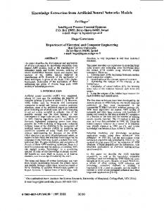
The fuzzy inference system performs a composition of the inputs using fuzzy set theory, fuzzy if-then rules and fuzzy reasoning to arrive at the output. More specifically, the fuzzy inference involves the fuzzification of the input variables (i.e. partitioning of the input data into fuzzy sets), evaluation of rules, aggregation of the rule outputs and finally the defuzzification (i.e. extraction of a crisp value which best represents a fuzzy set) of the result. There are two popular fuzzy models: the Mamdani model and the TS model. The TS model is more popular when it comes to data-driven identification and has been proven to be a universal approximator [6]. The TS model has been proven to have the ability to approximate any non-linear function arbitrarily well given that the number of rules is not limited. It is for these reasons that it is used in this study. The most common form of the TS model is the first order one. A diagram of a two-input and single output TS fuzzy model is shown in Figure 1:
Figure 1: An example of a two-input first order Takagi-Sugeno fuzzy model [7]. In the TS model, the antecedent part of the rule is a fuzzy proposition and the consequent function is an affine linear function of the input variables as shown in Eq. 1: Ri : If x is Ai then yi = aTi x + bi
(1)
where Ri is the ith fuzzy rule, x is the imput vector, Ai is a fuzzy set, ai is the consequence parameter vector, bi is a scalar offset and i = 1, 2, . . . , K. The parameter K is the number of rules in the fuzzy model. If there are too few rules in the fuzzy model, it may not be possible to accurately model a process. Too many rules may lead to an overly complex model with redundant fuzzy rules which compromises the integrity of the model [20]. In this work the optimum number of rules is empirically determined using a 10 fold cross-validation process. The optimum number of rules is chosen from the model with the lowest error and standard deviation. The final antecedent values in the model describe the fuzzy regions in the input space in which the consequent functions are valid. The first step in any inference procedure is the partitioning of the input space in order to form the antecedents of the fuzzy rules. The shapes of the membership functions of the antecedents can be chosen to be Gaussian or triangular. The Gaussian membership function of the form shown in Eq. 2 is used. i
µ (x) =
n Y
−
e
2 (xj −ci j) (bi )2 j
(2)
j=1
In Eq. 2, µi is the combined antecedent value for the ith rule, n is the number of antecedents belonging to the ith rule, c
is the center of the Gaussian function and b describes the variance of the Gaussian membership function. The consequent function in the TS model can either be constant or linear. In our work, it is found that the linear consequent function gives a more accurate result. The form of the linear consequent function is shown in Eq. 3: yi =
n X
pij xj + pi0
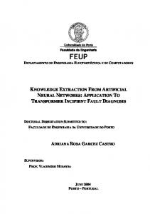
used as function approximators which map the inputs of a process to the outputs. The reason for their wide spread use is that, assuming no restriction on the architecture, neural networks are able to approximate any continuous function of arbitrary complexity [21]. A diagram of a generalised neural network model is shown in Figure 2.
(3)
j=1
where pij is the jth parameter of the ith fuzzy rule. If a constant is used as the consequent function, i.e. yi = pi , the zero-order TS model becomes a special case of the Mamdani inference system [7]. The output y of the entire inference system is computed by taking a weighted average of the individual rules’ contributions as shown in Eq. 4: PK y=
βi (x)yi Pi=1 K i=1 βi (x)
PK =
βi (x)(aTi x + bi ) PK i=1 βi (x)
i=1
(4)
Where βi (x) is the activation of the ith rule. The βi (x) can be a complicated expression but in our work it will be equivalent to the degree of fulfilment of the ith rule. The parameters ai are then approximate models of the non-linear system under consideration [1].
Figure 2: A diagram of a generalised neural network model The mapping of the inputs to the outputs using a MLP neural network can be expressed as follows: M X
yk = fouter
(2) wkj
d X
! (1) wji xi
+
(1) wj0
! +
(2) wk0
(5)
i=1
j=1
3.1.2. Neuro-fuzzy Modelling (1)
When setting up a fuzzy rule-based system we are required to optimise parameters such as membership functions and consequent parameters. In order to optimise these parameters, the fuzzy system relies on training algorithms inherited from artificial neural networks such as gradient descent-based learning. It is for this reason that they are referred to as neuro-fuzzy models. There are two approaches to training neuro-fuzzy models [7]: 1. Fuzzy rules may be extracted from expert knowledge and used to create an initial model. The parameters of the model can then be fine tuned using data collected from the operational system being modelled. 2. The number of rules can be determined from collected numerical data using a model selection technique. The parameters of the model are also optimised using the existing data. The Takagi-Sugeno model is most popular when it comes to this identification technique. The major motivation for using a neuro-fuzzy model in this work is that not only is it suitable for data-driven identification, it is also considered to be a gray box [1]. Unlike other computational intelligence methods, once optimised, it is possible to extract information which allows one to understand the process being modelled. In Section 4 we explore the interpretability of this model to see what kind of information can be explored. Later on in the work, the fuzzy model is proposed as a way of obtaining accurate forecasts and at the same time obtaining causal interpretations which are intuitive. The added advantage of this is that it is then easy to validate the model qualitatively using expert knowledge. 3.2. Neural Network Modelling This section gives an overview of neural networks and their practical implementation. Neural networks are most commonly
(2)
In Eq. 5, wji and wjk indicate the weights in the first and second layers, respectively, going from input i to hidden unit j, M is the number of hidden units, d is the number of output (1) (2) units while wj0 indicates the bias for the hidden unit j and wk0 indicates the bias for the output unit k. For simplicity the biases have been omitted from diagram in Figure 2. The weights of the neural network are optimised via back propagation training using, most commonly, scaled conjugate gradient training [22]. The cost function representing the objective of the training of the neural network can be defined. The objective of the problem to obtaining the optimal weights which accurately map the inputs of a process to the outputs. If the training set D = {xk , yk }N k=1 is used, the cost function, E, may be written using the cross-entropy cost function as follows [22]:
E = −β
N X K X n
k
ζ ln(ynk )+(1−tnk ) ln(1−ynk )+
w X αj 2 wj 2 j
(6) This cross entropy function has been chosen because it has been found to be more suited to classification problems that the sum-of-square of error cost function [22]. In Eq. 6, n is the index for the training pattern, hyperparameter β is the data contribution to the error, k is the index for the output units, tnk is the target output corresponding to the nth training pattern and kth output unit and ynk is the corresponding predicted output The second term in the expression is the regularisation parameter which penalises weights of large magnitudes. The regularisation parameter coefficient, α, determines the relative contribution of the regularisation term on the training error. The presence of the regularisation parameter gives significant improvements in the generalisation ability of the network [22]. The problem of identifying the weights and biases of the neural network can be posed in the Bayesian framework as shown in Eq. 7 [22].
P (D|w)P (w) P (w|D) = P (D)
(7)
In Eq. 7, P (w) is the probability distribution function of the weight-space in the absence of any data, also known as the prior distribution function and D ≡ (y1 , . . . , yN ) is a matrix containing the data. The quantity P (w|D) is the posterior distribution function after the network weights have been exposed to the data, P (D|w)) is the likelihood function and P (D) is the normalization function also known as the “evidence” [23]. For the MLP Eq. 7 may be expanded using the cross-entropy error function in Eq. 6 to give [22]: w
P (w|D) =
X αj 2 1 exp A + B − wj Zs 2 j
! (8)
Parameters Zs , A and B are described by the following equations: Z Zs (α, β) =
exp(−βED −αEw ) =
„
2π β
«N
„
2
+
2π α
«w 2
(9) A=β
N X K X n
ζ ln(ynk )
Table 1: The confusion matrix for the TS neuro-fuzzy model. The model classifies conflict with an accuracy of 80.6% Conflict cases Peace cases Correctly predicted 315 17967 Incorrectly predicted 77 8378
Table 2: The confusion matrix for the MLP neural network model. The MLP classifies conflict with an accuracy of 77.3% Conflict cases Peace cases Correctly predicted 303 19400 Incorrectly predicted 89 6945
4.2. Fuzzy rule Extraction The TS neuro-fuzzy model used for forecasting can also be used for rule extraction. Two fuzzy rules can be extracted from the model and they are shown below.
(10)
k
B = (1 − tnk ) ln(1 − ynk )
can be set. The single point on the ROC curve is usually termed the confusion matrix. The confusion matrices for both the TS neuro-fuzzy and Bayesian neural network models are shown in Tables 1 and 2, respectively.
(11)
From Eq. 8 we can see that training the neural network in the Bayesian framework automatically penalises overly complex models to without the need for cross-validation sets. This is especially an advantage if there are limited training examples. Equation 8 can be solved in two ways. The first way is by using Taylor expansion and approximating it by a Gaussian distribution and applying the evidence framework [24]. The second way, which is used in this work, is by numerically sampling the posterior probability using the Hybrid Monte Carlo method (HMC) [25]. The HMC method is a combination of the stochastic dynamics model adopted from statistical mechanics with the Metropolis algorithm. The HMC works by taking a series of trajectories from and initial state, i.e. ‘position’ and ‘momentum’, and moving in some direction in the state space for a given length of time and accepting the final state using the Metropolis algorithm. The algorithm makes use of gradient information to follow trajectories, which move in the direction of high probabilities, resulting in the improved probability that the resulting state is accepted. Further details of the HMC method can be found in Neal [25].
4. Knowledge Extraction 4.1. Classification Results The forecasting ability of the TS neuro-fuzzy and Bayesian neural network models are evaluated using ROC curves. Both the models are trained with a balanced training set containing 1000 instances. This is to ensure that both conflict and peace outcomes are given equal importance. The models are then tested on an the remaining unbalanced set which contains 26345 peace cases and 392 conflict cases. It is found that both perform similarly with areas under curve (AUC) of 0.82. By giving each dispute cases and non-dispute cases equal importance, an optimal threshold which corresponds to a single point on the ROC
1. If u1 is A11 and u2 is A12 and u3 is A13 and u4 is A14 and u5 is A15 and u6 is A16 and u7 is A17 then y1 = −1.86 · 10−1 u1 − 1.33 · 10−1 u2 + 0.00 · 100 u3 − 6.05 · 10−1 u4 − 1.26 · 10−1 u5 − 1.33 · 100 u6 + 4.71 · 10−1 u7 + 8.95 · 10−1 2. If u1 is A21 and u2 is A22 and u3 is A23 and u4 is A24 and u5 is A25 and u6 is A26 and u7 is A27 then y2 = −2.79·10−1 u1 +6.26·10−2 u2 +2.47·10−1 u3 − 7.56 · 10−1 u4 − 8.85 · 10−1 u5 − 9.04 · 100 u6 + 0.00 · 100 u7 + 3.73 · 10−1 The symbols from u1 to u7 are the input vector which consists of Democracy, Dependancy, Capability, Alliance, Contiguity, Distance and Major power. The rest of the symbols are as previously defined in Section It is clear that the rules are quite complex and need to be simplified in order to obtain a didactic interpretation. In fact it is often found that when automated techniques are applied to obtaining fuzzy models, unnecessary complexity is often present [20]. In our case the TS fuzzy model contains only two fuzzy rules. The removal of a fuzzy set similar to the universal set leaves only one remaining fuzzy set. This results in the input being partitioned into only one fuzzy set and therefore introduces difficulty when expressing the premise in linguistic terms. To simplify the fuzzy rules and avoid the redundant fuzzy sets the number of inputs into the TS neuro-fuzzy model have been pruned down to four variables. These variables are Democracy, Dependency, Alliance and Contiguity. Fig 3 illustrates how the output deteriorates when three of the inputs are pruned. The ROC curve shows that the performance degradation is minimal. The rules extracted can then be converted so that they are represented in the commonly used linguistic terms. However it is only possible to translate the antecedent of the fuzzy statement into English. The consequent part together with the
4.3. Automatic Relevance Determination and Sensitivity Analysis
Figure 3: A ROC illustrates the performance degradation of the neuro-fuzzy model when several inputs are pruned. The new AUC is now 0.74.
firing strength of the rule are still expressed mathematically. The translated fuzzy rules with the firing strengths omitted can be written as shown below.
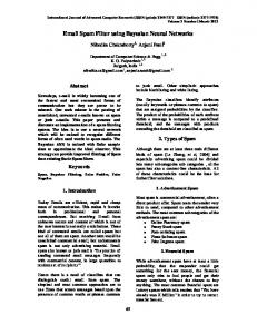
In this paper, the ARD is used to rank the 7 variables used in the analysis with regards to their relative influence on the MIDs. ARD is an extension of the Bayesian evidence framework. The ARD method uses the hyperparameters which control the magnitude of the weights assigned at the input layer of the neural network. The ARD was implemented, the hyperparameters calculated and then the inverse of the hyperparameters was calculated and the results are in Figure 4. Further details of the ARD method can be found in [4]. Figure 4 indicates that Dependency has the highest influence, followed by Capability, Democracy and then Allies. The remaining three variables, i.e. Contiguity, Distance and Major Power, have similar impact although it is smaller in comparison with other four variables. The results in Fig. 4 indicate that the two variables, Democracy and Dependency, have a strong impact on conflict and peace outcomes. However, Capability and Allies cannot be ignored. Once again this confirms recent positions, which see the Capability and Allies as mediating the influence of Democracy and Dependency by providing constraints or opportunities for state action [8, 17].
1. If Democracy level is low and Alliance is strong and Contiguity is true then y1 = −3.87·10−1 u1 −9.19·10−1 u3 −7.95·10−1 u4 + 3.90 · 10−1 2. If Democracy level is high and Alliance is weak and Contiguity is false then y2 = −1.25·10−1 u1 −5.62·10−1 u3 −2.35·10−1 u4 + 4.23 · 10−1
From observing the above rules, it is clear to see that the model is not quite as transparent as we would like it to be. This is because the consequent of each of the rules is still a mathematical expression. To validate the model we can then apply expert knowledge of the problem domain. For instance if the level of Democracy of two countries is low, they have a weak alliance and they share a border there is a reasonable chance that the countries can find themselves in a conflict situation. If we find values of Democracy, Alliance and Contiguity which have a membership value of one, we can then use these as inputs to the model to see if it confirms our existing knowledge. It is found that by using these values and and an arbitrary Dependency value the model gives a output decision value y = 0.6743. The output of the neuro-fuzzy model is determined as shown below: If y > Ts ⇒ conflict If y ≤ Ts ⇒ peace
(12)
The conflict threshold Ts is calculated from the ROC curve and is found to be 0.5360. By validating the model with similar statements, we can get a feel for how much confidence we can put in the system. The model can further be used to test hypothetical scenarios in a similar way to which it is validated. The neuro-fuzzy model therefore offers a method of forecasting international conflict while also catering for the cases where causal interpretations are required.
Figure 4: A graph showing the relevance of each variable with regards to the classification of MIDs. In sensitivity analysis we compare the model output with a new output produced by a modified form of the input pattern. When analysing the causal relationships between input and output variables, the neural network shows that when the Democracy variable is increased from a minimum to a maximum, while the remaining variables are set to a minimum, then the outcome moves from conflict to peace. This is an indication that although interactions exist, democracy also exerts a direct influence on peace. When all the variables were set to a maximum then the outcome was peace. When all the parameters were set to a minimum then the possibility of conflicts was 52%. These results are quite expected and indicate that all the inputs are quite important. When one of the variables was set to a minimum and the rest set to a maximum, then it was observed that the outcome was always peace. When each variable was set to a maximum and the remaining variables set to a minimum then the outcome was always conflict, with the exception of Democracy and Dependency where the outcome was peace. The first result stresses that strong interactions exist in relation to dispute patterns since no single low value can produce a dispute outcome. The second result indicates that more additive relationships than interactive ones are in place for peaceful patterns since one single maximum value for Democracy or Dependency
can maintain peace. These results support recent findings by Lagazio and Russett [17], but also reveal new insights. Democracy and Dependency emerge as having a strong additive impact on peace. This means that these two variables alone could contribute significantly to peace, even without the positive influence of the others.
5. Conclusion The transparency of both the Neuro-fuzzy and Neural Network models has been investigated. The models have been applied to the modelling of interstate conflict, an application in which obtaining causal interpretation of interstate interactions is just as important as forecasting dispute outcomes. The neural network, trained using the Bayesian framework, is found to offer some form of transparency. Knowledge can be extracted using Automatic Relevance Determination and also indirectly by performing a sensitivity analysis. The Takagi-Sugeno neuro-fuzzy model is also used to model interstate interactions. It is found that the model does offer some transparency, however it is limited due to the fact that the consequent of the fuzzy rules is expressed as a mathematical statement. In spite of this, the TS neuro-fuzzy model seems more suitable for hypothesis testing. A hypothesis stated linguistically can easily be verified using this model. In conclusion both models do offer transparency but the TS neuro-fuzzy model may be preferred as it easily verifies hypothetical scenarios expressed as linguistic statements.
6. References [1] R. Babuska, Fuzzy modeling and Identification. PhD thesis, Technical University of Delft, Delft, Holland, 1991. [2] D. Wang and W. Lu, “Interval estimation of urban ozone level and selection of influential factors by employing automatic relevance determination model,” Chemosphere, vol. 62, pp. 1600–1611, 2006. [3] A. Chamekh, H. BelHadjSalah, R. Hambli, and A. Gahbiche, “Inverse identification using the bulge test and artificial neural networks,” Materials Processing Technology, vol. 177, pp. 307–310, July 2006. [4] S. Papadokonstantakis, A. Lygeros, and S. P. Jacobsson, “Comparison of recent methods for inference of variable influence in neural networks,” Journal of Neural Networks, vol. 19, pp. 500–513, 2006. [5] T. Tettey and T. Marwala, “Controlling interstate conflict using neuro-fuzzy modeling and genetic algorithms,” in Proceedings of the IEEE International Conference on Intelligent Engineering Systems, (London, England), pp. 30–34, IEEE, 2006. [6] J. Jang, C. Sun, and E. Mizutani, Neuro-fuzzy and soft computing: A computational approach to learning and machine intelligence. New Jersey: Prentice Hall, first ed., 1997. [7] R. Babuska and H. Verbruggen, “Neuro-fuzzy methods for nonlinear sytem identification,” Annual Reviews in Control, vol. 27, pp. 73–85, 2003. [8] N. Beck, G. King, and L. Zeng, “Improving quantitative studies of international conflict: A conjecture,” American Political Science Review, vol. 94, no. 1, pp. 21–35, 2000. [9] C. Gochman and Z. Maoz, “Militarized interstate disputes 1816-1976,” Conflict resolution, vol. 28, no. 4, pp. 585– 615, 1984.
[10] “Correlates of war.” Internet Last Acessed: February 2006. http://www.correlatesofwar.org/.
Listing, URL:
[11] B. Russet and J. Oneal, Triangulating Peace: Democracy, Interdependence, and International Organizations. New York: W. W. Norton, J, 2001. [12] W. Thompson and R. Tucker, “A tale of two democratic peace critiques,” Journal of Conflict Resolution, vol. 41, no. 3, pp. 428–454, 1997. [13] E. D. Mansfield and J. Snyder, “A tale of two democratic peace critiques: A reply to Thompson and Tucker,” Journal of Conflict Resolution, vol. 41, no. 3, pp. 457–461, 1997. [14] J. Oneal and B. Russet, “The classical liberals were right: Democracy, interdependence and conflict, 1950-1985,” International Studies Quarterly, vol. 41, no. 2, pp. 267– 294, 1997. [15] K. Barbieri, “Economic interdependence - a path to peace or a source of interstate conflict,” Journal of Peace Research, vol. 33, no. 1, pp. 29–49, 1996. [16] N. Beck, J. Katz, and R. Tucker, “Taking time seriously: Time-series-cross-section analysis with a binary dependent variable,” American Journal of Political Science, vol. 42, no. 4, pp. 1260–1288, 1998. [17] M. Lagazio and B. Russett, A neural network analysis of MIDs, 1885-1992: Are the patterns stable? In the Scourge of War: New Extensions on an Old Problem, ch. Towards a Scientific Understanding of War: Studies in Honor of J. David Singer. Ann Arbor: University of Michigan Press, 2004. [18] T. Tettey and T. Marwala, “Controlling interstate conflict using neuro-fuzzy modeling and genetic algorithms,” in Proceedings of the 10th International Conference on Intelligent Engineering Systems, (London, England), pp. 30–34, IEEE, 2006. [19] C. Harris, C. Moore, and M. Brown, Intelligent control: Aspects of Fuzzy Logic and Neural Nets. Singapore: World Scientific Publishing, first ed., 1993. [20] M. Sentes, R. Babuska, U. Kaymak, and H. van Nauta Lemke, “Similarity measures in fuzzy rule base simplification,” IEEE Transactions on Systems, Man and Cybernetics-Part B: Cybernetics, vol. 28, no. 3, pp. 376– 386, 1998. [21] D. Tikk, L. T. K´oczy, and T. D. Gedeon, “A survey of universal approximation and its applications in soft computing,” Research Working Paper RWP-IT-2001. School of Information Technology, Murdoch University, Perth, 2001. [22] C. Bishop, Neural Networks for Pattern Recognition. New York: Oxford University Press, 1996. [23] D. MacKay, Bayesian methods for adaptive models. PhD thesis, California Institute of Technology, 1991. [24] D. MacKay, “A practical Bayesian framework for backpropagation networks,” Neural Computation, vol. 4, no. 3, pp. 448–472, 1992. [25] R. Neal, Bayesian Learning for Neural Networks. PhD thesis, Department of Computer Science, University of Toronto, Canada, 1994.