modelling of suspended sediment transport in ... - ARPN Journals

VOL. 12, NO. 16, AUGUST 2017

ISSN 1819-6608

ARPN Journal of Engineering and Applied Sciences ©2006-2017 Asian Research Publishing Network (ARPN). All rights reserved.

www.arpnjournals.com

MODELLING OF SUSPENDED SEDIMENT TRANSPORT IN COASTAL DEMAK INDONESIA BY USING CURRENTS ANALYZING Denny Nugroho Sugianto1, Sugeng Widada1, Anindya Wirasatriya1, Aris Ismanto1, Alfin Darari2 and Suripin3 1Department

of Oceanography, Diponegoro University, Semarang, Indonesia of Physics, Diponegoro University, Semarang, Indonesia 3Department of Civil Engineering, Diponegoro University, Semarang, Indonesia E-Mail: [email protected] 2Department

ABSTRACT Demak experienced severe abrasions in recent years and Demak coastal erosion has become a national issue. In this study we conducted through a case a study influence of ocean currents and soils structures abrassion. The study covered from 3 -10th June 2016 with ADCP to record 7 x 24 hours. The shear stress in the flow above a bottom-mounted ADCP is estimated from the difference of velocity variance in the opposing ADCP beams. The dynamics of current velocity and validation with current measurement using Sontek Argonaut observation, it was obtained a value of RMSE. The result is the highest flow velocity occurs at a depth of 6 m flow velocities ranging between 0098-0126 m / s east and 0114-0149 m / s north. The yield on the scatter plot shows that the predominant direction of the current is moving to the Northeast. Keywords: demak, Indonesia, modelling, sediment, transport.

INTRODUCTION Demak is one of the regencies in Central Java Province, Indonesia located in 6º43'26" - 7º09'43" S and 110027’58” - 110048'47" E. Demak has an area of ± 1.149,07 km² which consists of land of ± 897,43 km² and ocean of ± 252,34 km²[1]. Generally, the type of soil in Demak is alluvial soil that is susceptible to coastal erosion process [2]. Based on the data from the Environmental Impact Management Agency (Bapedal) of Central Java Province in 2008, Sayung district, Demak experienced severe abrasions in recent years and Demak coastal erosion has become a national issue. [3]. Provincial Development Planning Agency (Bappeda) report of Central Java Province in 2007, the coastal mangrove area in Central Java was 10.876 ha which 96, 9 of them were in damage. The area of the coastal mangrove continually fell into degradation, so that the result of the study of the coastal mangrove in 2014 only found 5.381,15 ha of ground cover vegetation [1]. There are a number of reasons for the abrassion that we are witnessing today. Coastal abrassion in Central Java Province is mainly influenced by natural processes such as crossshore and long-shore sediment movement and due to dynamic water levels at the coastal area, such as the wave action caused by winds, high tides due to astronomical tidal activity, and accelerated sea level rise due to global warming. In addition, coastal erosion may also give influence to shoreline change [3-5]. Type of soil on the north coast of Central Java Demak district in particular is the kind of alluvial soil that is susceptible to beach erosion processes [6]. Alluvial soil types derived

from flood sediment that is still young and there has been no differentiation horizon. Parent material derived from alluvium in the form of sand deposition. Alluvial soil type is characterized by slow soil permeability and has a high level of sensitivity to erosion [7]. This location is eroding coastal between 200-900 m over 10 years since 2003. In this study we conducted through a case a study influence of ocean currents and soils structures abrassion. The study covered from 3 -10th June 2016 with ADCP to record 7 x 24 hours. The shear stress in the flow above a bottom-mounted ADCP is estimated from the difference of velocity variance in the opposing ADCP beams [8 - 12] in a technique analogous to that used in stress measurements in radar meteorology. The dynamics of current velocity and validation with current measurement using Sontek Argonaut observation, it was obtained a value of RMSE [13]. METHODOLOGY This research was conducted in 4 research station locations spread in the waters of Timbulsloko Village, Demak by using the seabed geology and geomorphology parameters, and the nature of hydro oceanography current with measurements using waterpass. The method of collecting data for the ocean current was conducted by Euler methods; while for tidal current observation was conducted by the direct observation method. Before that a collecting data using Echosounder and tranducer instrument for record deept and morphology coastal in demak sayung Figure-1.

4666

VOL. 12, NO. 16, AUGUST 2017

ISSN 1819-6608



Figure-1. Contour of deept in Demak (source : Research study in 2016). Based Figure-1 deep measurement could represented in 3D Modelling for know a morfology of coastal. The ocean current measured using ADCP to record the current simultaneously and automatically. The measurement of the current had been conducted for 7 x 24 hours in one location representing the characteristic of the waters around Timbulsloko village, Demak. The analysis of hydro oceanography also had been equipped with the analysis of mathematical modeling to find out the characteristic of the physical properties of the waters spatially and temporally

(a)

RESULT AND DISCUSSIONS

(b)

Seabed geology and morphology The measurement of deept presented using interval 0.5 m get a deep value and map interval untill 2.5m at 2 km from coastline. Result in 3D modelling Value of slope present from near using declitivy ratio (c)

(d) Figure-3. Declitivy in different location 1(a) location 2 (b) Location 3(c) location 4 (source : Research study in 2016). Figure-2. Contour 3D modelling of deep in Demak (source : Research study in 2016). and different height [14]. A cross section obtain value of declivity shows that Figure-3, Figure-7.

Figure-3 Shows a value of declitivy in different location that represented location in demak, this location flat and gently slope, it cause comparison of angle of slope average 0 - 2% and range height below 5 m. The measurement of current data used ADCP direct observation instrument (coordinates 6.890034629° S

4667

VOL. 12, NO. 16, AUGUST 2017

ISSN 1819-6608


www.arpnjournals.com and 110.45185° E) shown in Figure-1, the data then was processed using euler methods in Sayung district, Demak around the Java Sea area. The period of the current recording (direction and velocity) and wave (height and period) ran simultaneously and automatically from 3-10 June 2016. From the data, the dominant current from various depths is obtained. The data are scatter plot; stick diagram, currentrose, Vertical current velocity. The average velocity of the ocean current using ADCP measurements was about from of June 3rd, 2016 at 11:00 pm until June 10th, 2016 at 18:40 pm.

(a)

(b) Figure-6. The pattern of ocean currents a) a scatter plot, b) stick diagram depth of 6 meters. Figure-4. Study area and field ADCP intrumentation sites for measurement wave and current. Study of current The current plot at a depth of 8m, 6m, 4m, 2m and the surface current would show a different direction and velocity. The Scatter plot value of the ellipse ocean current data processing illustrates the dominant direction of the ocean current [15].

(a) Figure-7. The pattern of ocean currents a) a scatter plot, b) stick diagram depth of 4 meters. (b) Figure-5. The pattern of ocean currents a) a scatter plot, b) stick diagram depth of 8 meters.

4668

VOL. 12, NO. 16, AUGUST 2017

ISSN 1819-6608



Figure-8. The pattern of ocean currents a) a scatter plot, b) stick diagram depth of 2 meters.

the depth of 6 meters was more concentrated in the northeast. At the depth of 4 m the current velocity ranged between 0102-0115 m / s to the east and 0074-0132 m / s to the north (Figure-7), current direction at the depth of 4 meters was more concentrated in the northeast. At the depth of 2 m the current velocity ranged 0.066-0.1m / s to the east and 0078-0147 m / s to the north a results of the plot can be seen in Figure-8 current direction at the depth of 2 meters was more concentrated in the northeast. At a depth of 2 m the current velocity ranged 0.066-0.1m / s to the east and 0078-0147 m / s to the north. The results of the plot can be seen in. The current direction at the depth of 2 meters was more concentrated in the northeast. The current velocity measured on the surface ranged from 0.105-0.093m / s to the east and 0.062-0.1123 m / s to the north. The results of the plot can be seen in Figure-9 current direction at a depth of 2 meters was more concentrated in the Northeast. The result on the scatter plot shows that the predominant direction of the current moves to the Northeast Figure-10. Value of differences of the current pattern on the surface with a Vertical current velocity were influenced by internal factors and external factors. A Research conducted by Widyastuti [16] stated that the movement of the ocean surface current follows the direction of the wind. Hoitink et al [17] reported in wishes [18] that the surface current is influenced by monsoons. June is an East monsoon. Surface current rose shows the direction that almost same with the direction of the wind. The current moves toward the Northeast at a speed of 0:04 to 0:12 m / s. A stick diagram illustrates that the direction of current movement tends to commute due to the influence of the tidal current [19]. In principle, the result of a stick diagram process is same with the scatter plot diagram which illustrates that the current velocity in the waters of Sayung district is relatively small. So is the dominant direction of the ocean current to the East. Current that occurs in shallow waters and calm waters has characteristic in a current with a speed that is not so big [20]. A vertical movement of ocean currents at each depth can be determined by the current vertical profile (Figure 10 a, b and c) showing that the deeper the waters is, the weaker current speed will be, caused by the influence of the basic friction and the influence of density.

Figure-9. The pattern of ocean currents surface a) a scatter plot, b) Stick diagram. At the depth of 8 m the current velocity ranged between 0095- 0115 m / s to the east and 0059-0122 m / s to the north. domination of the direction was to the Southeast and Northwest, result of the plot is shown in figure 5. At the depth of 6 m the current velocity ranged between 0098-0126 m / s to the east and 0114-0149 m / s to the north can be seen in Figure-6. Current direction at

4669

VOL. 12, NO. 16, AUGUST 2017

ISSN 1819-6608



(d) (a)

(e) (b)

Figure-10. Current rose in different condition (a) 8m deept (b) 6m deept (c) 4m deept (d) 2m Deept (e) surface area.

(c)

4670

VOL. 12, NO. 16, AUGUST 2017

ISSN 1819-6608


www.arpnjournals.com density so that the energy generated by the current is very weak and the hampered current movement makes the current more regular. In contrast to current on surface area is much influenced by wind and tidal. Thus, pattern and current velocity will be more random and faster.

(a)

(b)

Characteristics of sediment Sediment statistics from sediment are the value of Median, Mean, Sortation, Skewness and Sharpness are obtained from shieve graph plot representing the size of grains and percentage of retained sediment weight. The relations between the value of median and mean of sediment are shown in the Figure-12. The highest median value on station 1 that is located in the mouth of Sayung River. Station 4, 5, 6, 7 and 8 that is located in Timbulsloko Village has the same median value. The lowest median and mean values are obtained from the sediment footage on station 3 of 0.15 in each.

Figure-12. Graph of mean and median at location. The sortation classifications obtained from each station are shown on Figure-12. Sediment footage sortation included in the category of Excellent was obtained from station 3, 5, 6, 7, 8 and 9. Meanwhile, station 1, 2, 4 have the sortation category of Very Good skewness.

(c) Figure-11. Current velocity (a) East, (b) North dan (c) Up Velocity. The deeper the water is, the bigger the density and the smaller the current speed will be. It is same with Jantama [15] study (2015) on the shallow pond the current movement is not significant due to its basic friction and

Figure-13. Graph of skewness at station. The skewness classification is calculated on station 3, 6, 7 and 8, positive on station 9 and a strong positive skewness scoring category are calculated on station 1, 2, 4 and 5.

4671

VOL. 12, NO. 16, AUGUST 2017

ISSN 1819-6608



Figure-14. Graph of kurtosis at station.

The results of the analysis of grain size from all of the stations get non- cohesive sediment type (Station 1, 5, 6, 7 and 9) and cohesive sediment (Station 2, 3 and 4). The waters have type of sloping landform. Non-cohesive sediment (minimum sand grain size) along the swash zone will move and pass through the breaking wave zone and then head to deeper waters [21]. Cohesive sediment is very easy to agglomerate and then the subsequent flocculation mechanism depends on the salinity levels, this agglomerate process will move and affect the sediment classification and its characteristics [22].

Figure-15. Sayung district rivers map. Sediment supply Sediment supplies were obtained from several river streams that flow into the waters. The sampling location can be seen in Figure-15 on Sayung District Rivers Map.

The distribution of sampling was divided on each sediment supply flows within each rivers were taken three sampling locations, which were in the estuary, adjacent to the north coast and the middle around. The sampling location and the value of width and depth can be seen on Table-1 River and its Size.

4672

VOL. 12, NO. 16, AUGUST 2017

ISSN 1819-6608


www.arpnjournals.com Table-1. River and characteristic. River

Sayung

Daleman

Onggoraw e

-6.924180°

Depth (meter) 1.5

Wide (meter) 67.37

110.495060°

-6.932750°

1.0

23.07

S3

110.502620°

-6.939860°

1.5

12.54

S4

110.495356°

-6.904206°

1.5

15.27

S5

110.514852°

-6.917993°

1.0

9.01

S6

110.533470°

-6.933300°

1.5

5.62

S7

110.508208°

-6.884803°

1.8

76.07

S8

110.526280°

-6.904220°

1.5

10.36

S9

110.537509°

-6.925162°

1.1

10.04

Sample

Longitude

Latitude

S1

110.479230°

S2

The result of the analysis of water bottoms sediment grain obtained on 6 locations are shown in Table-2 Based on the result of analysis of grain size, it is known that in all sampling locations the sediments are silt with the percentage of silt are more than 90% and the rests are clay. This condition indicates that the sediments in the study area are transported more as a suspended solid load than a basic load. This fact is in accordance with the field condition where the sea water is very turbid.

Characteristics of hydrodynamics The information about the hydrodynamics in waters is used as a forecasting and mitigation in coastal area. In order to obtain a picture of hydrodynamics of waters, the field measurement and calculation is needed to be done. However, in a large area, it is hard to be done because of the limited time. To solve the problem a numerical modeling is being done. One of current numerical modeling 2D that exists is current modelling. In theory, this modeling uses the law of momentum conservation and water mass. The application of the equation is able to calculate the density, depth and the generator force of current circulation generated by the tides [23].

4673

VOL. 12, NO. 16, AUGUST 2017

ISSN 1819-6608


www.arpnjournals.com Table-2. Analysis of sediment grain. Grain size

% Weight

% Cumulative

Grain size classification ( % )

Sediment

Location 1 Morosari village 0.0625

48.24

48.24

0.0312

29.41

77.65

0.0156

14.12

91.76

0.0078

2.35

94.12

0.0039

5.88

100.00

Silt

94.12

Clay

5.88

Silt

Location 2 Timbulsloko village 0.0625

40.41

40.41

0.0312

34.20

74.61

0.0156

21.24

95.85

0.0078

3.11

98.96

0.0039

1.04

100.00

Silt

98.06

Clay

1.04

Silt

Location 3 Surodadi village 0.0625

31.07

31.07

0.0312

33.01

64.08

0.0156

30.10

94.17

0.0078

3.88

98.06

0.0039

1.94

100.00

Silt

98.06

Clay

1.94

Silt

Location 4 Estuary Kontrak 0.0625

43.00

43.00

0.0312

37.00

80.00

0.0156

14.50

94.50

0.0078

4.50

99.00

0.0039

1.00

100.00

Silt

99.00

Clay

1.00

Silt

Location 5 Surodadi village 0.0625

38.89

38.89

0.0312

31.94

70.83

0.0156

18.06

88.89

0.0078

6.94

95.83

0.0039

4.17

100.00

Silt

95.83

Clay

4.17

Silt

Location 6 Bonang river 0.0625

37.20

37.20

0.0312

35.75

72.95

0.0156

23.19

96.14

0.0078

2.90

99.03

0.0039

0.97

100.00

The result of the current velocity hydrodynamic model with the water conditions scenario in 7 days (3-6 June 2016) were 188 time step, which can be seen on Figure-15. The current velocity on the modeling area was decreasing on the shallower area or close to the coastal

Silt

99.03

Clay

0.97

Silt

area. In research location, the current velocity fluctuation was 0,005 to 0,090 m/Sec. The dynamics of current velocity and validation with current measurement on field can be seen in Figure16. Based on the validation between models and ADCP

4674

VOL. 12, NO. 16, AUGUST 2017

ISSN 1819-6608


www.arpnjournals.com Sontek Argonaut observation, it was obtained a value of

RMSE 3, 93. Current direction and speed is in Figure-16.

Figure-16. Modelling of hydrodynamics.

Figure-17. Observation of modelling current velocity.

4675

VOL. 12, NO. 16, AUGUST 2017

ISSN 1819-6608



Figure-18. Modelling of current. Modelling of transport sediment Effects tidal currents, waves generated by wind, the grain size of the sediment, stream sediment, thickness of bottom sediments taken into modelling of sediment transport. In shallow water area when the wave height increased flow velocity will increase. Sediment classification sludge will accumulate in the intertidal zone,

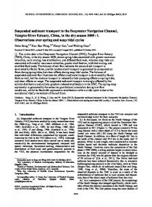
while the sand will be distributed in deeper waters, but when there is a strong wave of the sediment (sand and silt) stirred and eroded [22]. The result of the current velocity hydrodynamic model with the water conditions in 7 days ( 3-6 June 2016) get a value bed level transformation shows that Figure-18.

Figure-19. Modelling of transport sediment. Result of modelling transport sediment using current modelling software (Figure-19) acquire Bed Change Level at point 1 highest point 2 and 3. After 7 days, at 1 point going seabed thick accretion of 0.16 mm, 0.02 mm thick point 2 and point 3 is 0.005 mm thick. Point 1 is located at the river mouth, point 2 on offshore and point 3 in Timbulsloko waters with a depth of less than 1 m. Circulation of sediment near the beach and the mouth of the river is very influenced by the seasons and

conditions are always changing, it is happening at low latitudes [24].

4676

VOL. 12, NO. 16, AUGUST 2017

ISSN 1819-6608


www.arpnjournals.com ACKNOWLEDGEMENTS We would like to thank to the Lembaga Penelitian dan Pengabdian kepada masyarakat (LPPM) Diponegoro University and Center for Coastal Disaster Mitigation and Rehabilitation Studies (PKMBRP), Diponegoro University. Thanks also to all the respondents, the village chiefs, and all those who have helped so done research. REFERENCES Figure-20. Graph of transformation modelling thickness land.

[1] Marfai MA. 2011. The hazards of coastal erosion in Central Java, Indonesia: An overview. Malaysia Journal of Society and Space. 7(3): 1- 9. [2] Badan Pusat Statistik. 2012. Kecamatan Dalam Angka. Demak. [3] Bagli S, Soille P. 2003. Morhological automatic extraction of Pan-European coastline from Landsat ETM+images. International Symposium on GIS and Computer Cartography for Coastal Zone Management, October, Genova.

Figure-21. Graph of current velocity significant. Graph velocity flow hydrodynamic modeling results presented in Figure-21. At the point 1, 2 and 3 the highest flow velocity occurs at point 2 (located off the coast) to reach 0.37 m / s, the flow velocity at point 1 and 3 are located near the beach ranged from 0.03 to 0.18 m / sec. Speed affects the flow of sediment concentration due to interactions produce different concentrations of sediment concentrations in the water bottom [25]. Displacement of sediment that slowly changes the condition of the coastline is a sediment transport mechanisms are directly affected by waves and currents [26]. Forecast sediment transport and connection with seasonal variations can be obtained from the wave data per season. On a large scale would result in the evolution of the coastline [27]. CONCLUSIONS The speed and direction of currents at each layer depth of 8m, 6m, 4m, 2m and surface currents indicate the direction and at different speeds. The highest flow velocity occurs at a depth of 6 m flow velocities ranging between 0098-0126 m / s east and 0114-0149 m / s north. The yield on the scatter plot shows that the predominant direction of the current is moving to the Northeast. Displacement of sediment that slowly change the condition of the coastline is a sediment transport mechanisms are Directly affected by waves and currents.

[4] Marfai MA, Almohammad H, Dey S, Susanto B, King L. 2008. Coastal dynamic and shoreline mapping: Multi-sources spatial data analysis in Semarang, Indonesia. Environmental Monitoring and Assessment. 142, pp. 297-308. [5] Supriharyono. 1990. Hubungan Tingkat Sedimentasi dengan Hewan Mikrobentos di Perairan Muara Sungai Moro Demak Kabupaten Dati II Jepara. Lembaga Penelitian Universitas Diponegoro. Semarang. [6] Stacey M. T., G. Monismith and J. R. Burau. 1999. Measurements of Reynolds stress profiles in unstratified tidal flow. J. Geophys. Res. 104, 10 93310 949. [7] Selley R. C. 1988. Applied Sedimentology. Academic Press. San Diego. [8] Stacey M. T., G. Monismith and J. R. Burau. 1999: Measurements of Reynolds stress profiles in unstratified tidal flow. J. Geophys. Res. 104, 10 93310 949. [9] Lu Y., R. G. Lueck and D. Huang. 2000. Turbulence characteristics in a tidal channel. J. Phys. Oceanogr. 30, 855-867. [10] Rippeth T. P., E. Williams and J. H. Simpson 2002: Reynolds stress and turbulent energy production in a tidal channel. J. Phys. Oceanogr. 32, 1242-125.

4677

VOL. 12, NO. 16, AUGUST 2017

ISSN 1819-6608


www.arpnjournals.com [11] Howarth M. J. and A. J. Souza. 2005: Reynolds stress observations in continental shelf seas. Deep-Sea Res. II, 52, 1075-1086. [12] Williams E. and J. H. Simpson. 2004: Uncertainties in estimates of Reynolds stress and TKE production rate using the ADCP variance method. J. Atmos. Oceanic Technol. 21, 347-357. [13] Muste Marian. kim, won and Fulford M., Janice. 2008. Developments in hydrometric technology: new and emerging instruments for mapping river hydrodynamics. WMO Bulletin. 57(3): 163-169. [14] Soewarno. 1991. Hidrologi Pengukuran dan Pengelolaan Data Aliran Sungai. Penerbit Nova. Bandung. [15] Witt, Gary. 2013. Using Data from Climate Science to Teach Introductory Statistics. Journal of Statistics Education. 21(1): 1-24. [16] Widiastuti R. 2010. Pemodelan Pola Arus Laut Permukaan Di Perairan Indonesia Menggunakan Data Satelit Altimetri Jason-2 Periode 2002-2009. Surabaya: Faculty of Engineering, ITS. [17] Hoitink A. J. F., Hoekstra P. & Van Maren D. S. 2003. Flow Asymmetry Associated with Astronomical Tides: Implication for the Residual Transport of Sediment. Journal of Geophysical Research. 108, 3315.

[22] Hou Z., Coco G., van der Wegen M., Gong Z., Zhang C. & Townend I. 2015. Modeling sorting dynamics of cohesive and non-cohesive sediments on intertidal flats under the effect of tides and wind waves. Continental Shelf Research. [23] Hakim B. Al et al. 2015. Hydrodynamics Modeling of Giant Seawall in Semarang Bay. Procedia Earth and Planetary Science. 14, pp. 200-207. [24] SP Chempalayil, VS Kumar, GU Dora, G Johnson. 2014. Near shore waves, long-shore currents and sediment transport along micro-tidal beaches, central west coast of India. International Journal of Sediment Research. 29(3): 402-413. [25] Cartier A & Héquette A. 2015. Variation in longshore sediment transport under low to moderate conditions on barred macrotidal beaches. Journal of Coastal Research, Special Issue 57, 2011. [26] Lu Y. et al. 2015. Advances in sediment transport under combined action of waves and currents. International Journal of Sediment Research. [27] Splinter K.D. et al. 2012. Climate controls on longshore sediment transport. Continental Shelf Research. 48, pp. 146-156.

[18] Wisha, Jantama Ulung. Husrin, Semeidi. Prihantono, Joko. 2016. Hydrodynamics Banten Bay during Transitional Seasons (August-September) (Hidrodinamika Perairan Teluk Banten Pada Musim Peralihan (Agustus–September)). LMU KELAUTAN. Juni 2015. 20(2): 101-112. [19] Lacoste N., Karine. Munro, Jean, Castonguay Martin, Saucier Francois J, Gagne Jacques A. 2001. The influence of tidal streams on the pre-spawning movements of Atlantic herring, Clupea harengus L., in the St Lawrence estuary. Journal of Marine Science. 58: 1286-1298. [20] Triatmodjo B. 1999. Teknik Pantai. Beta Offset. Yogyakarta. [21] Bayram A., Larson M. & Hanson H. 2007. A new formula for the total longshore sediment transport rate.

4678