Hydrol. Earth Syst. Sci., 19, 195–208, 2015 www.hydrol-earth-syst-sci.net/19/195/2015/ doi:10.5194/hess-19-195-2015 © Author(s) 2015. CC Attribution 3.0 License.
Monitoring of riparian vegetation response to flood disturbances using terrestrial photography K. Džubáková1,2 , P. Molnar1 , K. Schindler3 , and M. Trizna2 1 Institute
of Environmental Engineering, ETH Zurich, Switzerland of Physical Geography and Geoecology, Comenius University in Bratislava, Slovakia 3 Institute of Geodesy and Photogrammetry, ETH Zurich, Switzerland 2 Department
Correspondence to: P. Molnar (
[email protected]) Received: 3 March 2014 – Published in Hydrol. Earth Syst. Sci. Discuss.: 21 March 2014 Revised: 5 November 2014 – Accepted: 12 November 2014 – Published: 13 January 2015
Abstract. Flood disturbance is one of the major factors impacting riparian vegetation on river floodplains. In this study we use a high-resolution ground-based camera system with near-infrared sensitivity to quantify the immediate response of riparian vegetation in an Alpine, gravel bed, braided river to flood disturbance with the use of vegetation indices. Five large floods with return periods between 1.4 and 20.1 years in the period 2008–2011 in the Maggia River were analysed to evaluate patterns of vegetation response in three distinct floodplain units (main bar, secondary bar, transitional zone) and to compare the sensitivity of seven broadband vegetation indices. The results show both a negative (damage) and positive (enhancement) response of vegetation within 1 week following the floods, with a selective impact determined by pre-flood vegetation vigour, geomorphological setting and intensity of the flood forcing. The spatial distribution of vegetation damage provides a coherent picture of floodplain response in the three floodplain units. The vegetation indices tested in a riverine environment with highly variable surface wetness, high gravel reflectance, and extensive water–soil– vegetation contact zones differ in the direction of predicted change and its spatial distribution in the range 0.7–35.8 %. We conclude that vegetation response to flood disturbance may be effectively monitored by terrestrial photography with near-infrared sensitivity, with potential for long-term assessment in river management and restoration projects.
1
Introduction
Riparian vegetation is under natural conditions a dynamic component of the riverine environment, which together with floodplains and river marginal wetlands provides a range of important ecosystem services such as biodiversity, flood retention, nutrient sink, pollution control, groundwater recharge, timber production, and recreation (e.g. Tockner et al., 2008). The species composition and spatial distribution of riparian vegetation is largely determined by floodplain morphology and river flow regime (e.g. Bendix and Hupp, 2000; Merritt et al., 2010; Gurnell et al., 2012) as well as by plant tolerance and response to flood disturbance and water stress (e.g. Auble et al., 1994; Blanch et al., 1999; Glenz et al., 2006; Pasquale et al., 2012). The reciprocal interactions between hydromorphological processes and riparian vegetation lead on the long term to the formation of complex mosaics of landforms and their respective biological communities and habitat patches (e.g. Pringle et al., 1988; Gregory et al., 1991; Decamps, 1996; Latterell et al., 2006; Gurnell and Petts, 2006; Corenblit et. al., 2007; Gurnell and Petts, 2011). The impact of floods on riparian vegetation is well documented in the literature. The most apparent is a direct negative impact when the vegetation is scoured (Bendix, 1999; Edmaier et al., 2011; Crouzy et al., 2013), covered by sediment and debris (Ballesteros et al., 2011), drowned (Friedman and Auble, 1999), or where it looses its connection to the water table due to channel displacement (Loheide and Booth, 2011). A less evident negative impact of floods is a general decrease in vegetation vigour associated with the post-stress reaction of plants. Plants under flood-induced stress have both short-term and long-term physiological and
Published by Copernicus Publications on behalf of the European Geosciences Union.
196
Džubáková et al.: Monitoring riparian vegetation response to flood disturbances
morphological responses (Kozlowski and Pallardy, 2002), such as root mortality or reduced photosynthetic activity, plant growth, dry matter production, and reproduction (e.g. Hatfield, 1997; Toda et al., 2005). However, floods can positively influence riparian vegetation by generation of new germination sites, by distribution of propagules and woody debris (Gurnell and Petts, 2006; Bertoldi et al., 2011a; Gurnell et al., 2012), and by enabling access to water and nutrients in usually disconnected parts of the floodplain (Amoros and Bornette, 2002). Some of these relationships have been replicated in flume experiments (e.g. Tal and Paola, 2010; Perona et al., 2012) and used in numerical modelling (e.g. Perona et al., 2009a, b). The monitoring of riparian vegetation in floodplains can be achieved by a range of sensors and methods (see review in Carbonneau and Piégay, 2012). Changes in riparian vegetation cover at the large scale are commonly quantified with remotely sensed data, such as satellite imagery (Verrelst et al., 2008; Johansen et al., 2010; Bertoldi et al., 2011a, b; Caruso et al., 2013; Parsons and Thoms, 2013) and aerial photography (e.g. Bertoldi et al., 2011a, b; Mulla, 2012). These are usually suitable for applications to large rivers at irregular time sampling. More recently, unmanned aerial vehicles (UAVs) have been used for monitoring with high resolution and large coverage, at a sampling rate determined by user (Berni et al., 2009; Dunford et al., 2009; Zhang and Kovacs, 2012). Another approach for detailed local analysis of riparian vegetation is terrestrial photography. Consumer grade cameras have recently been successfully used for monitoring plant conditions and phenology (e.g. Sakamoto et al., 2012; Sonnentag et al., 2012; Petach et al., 2014; Nijland et al., 2014). Similarly to UAV systems, terrestrial photography has the advantage of a high spatial resolution and a user-defined regular high sampling rate. In addition, terrestrial photography by fully automatic systems has minimal running costs after installation. Disadvantages are a restricted areal coverage and limits of oblique photography (e.g. Morgan et al., 2010; Crouzy et al., 2013). Since we study short-term floodplain response to floods we have opted for terrestrial monitoring by cameras, where we can obtain images shortly before and immediately after large flood events. Our photographic monitoring system records the imagery of a gravel bar in the visible and near-infrared range that is processed into broadband vegetation indices. Broadband and narrowband vegetation indices (VIs) are standard methods used in remote sensing to identify vegetation and quantify properties such as leaf surface pigmentation, photosynthetic activity, and canopy structure. The detailed overview of VIs and their applications is well explained in the literature (e.g. Jones and Vaughan, 2010). The choice of a suitable vegetation index depends on target plant attributes (Sims and Gamon, 2003; Ortiz et al., 2011; Bargain et al., 2013), environment settings (Barati et al., 2011), and available spectral bands (Adam et al., 2010). In this study we Hydrol. Earth Syst. Sci., 19, 195–208, 2015
have used a selection of the most common broadband indices (Table 1). The main aims of this study are (1) to analyse the spatial distribution and intensity of the vegetation response to large floods, where we aim to capture not only severe vegetation damage and scouring, but also less apparent change of vegetation vigour; (2) to study the differences in vegetation response to floods in three distinct floodplain units (main bar, secondary bar, transitional zone), which are meaningful units with regard to the concept of the floodplain mosaic system; and (3) to study differences in the performance of several vegetation indices in identifying the direction and magnitude of floodplain change. The analysis was performed for five floods in a 4-year period (2008–2011) on a gravel bar of an Alpine braided river (Maggia River, Switzerland). The relatively numerous flood events within the 4 study years enabled us to assess the vegetation response of the same species composition to different flood stages and longer-term weather conditions. The novelty of this work lies in (a) the use of near-infrared (NIR) sensitive camera monitoring of a complex alluvial system consisting of water, sediment and vegetated surfaces; (b) high spatial resolution of the images which allows identifying individual plants; and (c) continuous (daily) monitoring which allows for the spatial analysis of the short-term response before and after individual large floods in terms of both vegetation enhancement and damage.
2
Study area
Maggia is an Alpine river located in southeastern Switzerland, north of the city of Locarno. The river originates at an altitude of about 2500 m and flows south through the Maggia Valley into Lake Maggiore (193 m). The bedrock of the valley is formed by Penninic crystalline nappe predominantly covered by Holocene alluvial deposits. Within these settings Maggia evolved into a braided river system with a gravel cobble bed occasionally covered with fine sand sediment deposits on elevated alluvial bars. The average bed slope in the main valley is about 0.8 %. The hydrological regime of the river is significantly influenced by hydropower infrastructure (dams, intakes, canals) constructed in the upper watershed in the 1950s. Since then, approximately 75 % of the natural river flow has been diverted to the power station Verbano at Lake Maggiore and only minimum flows are released into the main valley. At present, the bypassed section has an average daily streamflow of 4.1 m3 s−1 , while it was close to 16 m3 s−1 prior to 1954 (Molnar et al., 2008). The 100-year flood peak is estimated at 768 m3 s−1 (Bignasco) at the upper end of our study reach. The hydropower system regulation practically removes the snowmelt spring–summer flow peak in the valley, but does not affect the largest floods appreciably, mainly due to the upstream location of reservoirs and their relatively low storwww.hydrol-earth-syst-sci.net/19/195/2015/
Džubáková et al.: Monitoring riparian vegetation response to flood disturbances
197
Table 1. Overview of the VIs used in this study. NIR, R, and G stand for the spectral reflectance in the near-infrared, visible red and visible green frequencies. L is a scaling constant (here L = 0.5).
RVI GRVI NDVI GNDVI SAVI GSAVI CVI
Vegetation index
Formula
Reference
Red VI Green ratio VI Normalized difference VI Green normalized difference VI Soil adjusted VI Green soil adjusted VI Chlorophyll VI
NIR/R NIR/G (NIR − R)/(NIR + R) (NIR − G)/(NIR + G) (1 + L)(NIR − R)/(NIR + R + L) (1 + L)(NIR − G)/(NIR + G + L) NIR · R/G2
Birth and Mcvey (1968) Sripada et al. (2008) Rouse et al. (1974) Gitelson et al. (1996) Huete (1988) Sripada et al. (2008) Vincini et al. (2008)
age capacity. As a consequence, floods with a perceptible impact on riparian vegetation still occur on average more than once per year in the main valley (Perona et al., 2009a). In this study we focused on the 500 m long and 300–400 m wide reach of the river in the main valley located between the villages Someo and Giumaglio. Three distinct floodplain units within the study reach were identified, namely main gravel bar (MB), secondary gravel bar (SB), and transitional zone (TZ) (Fig. 1). The units were delineated based on the floodplain morphology identification of river banks using a LiDAR (light detection and ranging) DEM (digital elevation model) of 2004 and image quality (the marginal zones of the floodplain were excluded due to the interference of surrounding forest). The main bar is the largest, most elevated unit. It is located in the centre of the floodplain in close proximity to the main channel. The secondary bar is at the edge of the floodplain. Both bars are separated by the transitional zone with very active channel dynamics. The secondary channel in the transitional zone is fully connected with the main channel only during flood events. The vegetation composition within the study reach is heterogeneous (Fig. 2). The dominant willows (Salix species) are Salix purpurea, Salix alba, Salix eleagnos, often accompanied by poplars (Populus nigra) and alders (Alnus incana), occasionally by maples (Acer pseudoplatanus), lindens (Tilia cordata), knotweeds (Fallopia sachalinensis), and locusts (Robinia pseudoacacia). The tree height varies from 1 to 10 m. Sparse herbaceous cover grows sporadically on the inner part of the bars with sand accumulation. The variability in the vegetation composition within the three studied floodplain units is notable. Salix individuals are located at the upstream part of MB, and towards its inner part are often accompanied by Populus. Unlike on MB, Salix is predominantly mixed with Fallopia on SB. Although fewer in number, the largest diversity in species is found in TZ with Alnus, Salix, locally Populus and Acer.
www.hydrol-earth-syst-sci.net/19/195/2015/
3 3.1
Data and methods Meteorological and hydrological data
Hourly records of solar radiation, air temperature, relative humidity, and rainfall used in this study were obtained from the weather station Locarno-Monti (MeteoSwiss – Federal Office of Meteorology and Climatology), located about 15 km downstream from the study reach. Hourly streamflow is gauged on the Maggia River at Bignasco, Ponte Nuovo station (FOEN – Federal Office for the Environment), approximately 7.8 km upstream of the study reach. There is an ungauged small tributary (Rovana) between the gauging station and our study reach; thus, the reported peak flows of the studied floods in our reach are a lower estimate. We analysed the five largest summer floods occurring between 2008 and 2011 with return periods between 1.4 and 20.1 years (Table 2). The flood in 2008 submerged the upstream and middle part of the MB and the whole TZ; more voluminous floods in 2009 and 2010 progressed further and submerged the TZ and the majority of the bars. The most elevated areas of the MB and SB were submerged only in 2011. We defined the duration of the floods based on the discharge when the river inundates the predominantly unvegetated floodplain (180 m3 s−1 ). The flood peaks of the first four floods exceeded a discharge of 180 m3 s−1 once for several hours; thus, they are considered to be single-peak floods. The flood in 2011 consisted of two flood peaks greater than 180 m3 s−1 over a period of 5 days. The meteorological conditions and streamflow before and after each flood are summarized in Fig. 3. The flood in May 2008 was the earliest in the season with the lowest air temperature (minimum 10 ◦ C) and the highest relative humidity prior to the event. The rain gauge at Locarno-Monti did not capture the storm rainfall which occurred mostly in the headwaters of the catchment. With the flood peak of 192 m3 s−1 , it was the smallest but at the same time the longest flood analysed. There were two floods with similar peaks in 2009. The summer of 2009 was very dry and hot, air temperatures prior to both floods reached or exceeded 30 ◦ C, relative humidity was generally very low. The flood in June had intense rainfall (40 mm h−1 ) measured in Locarno-Monti and the flood peak Hydrol. Earth Syst. Sci., 19, 195–208, 2015
198
Džubáková et al.: Monitoring riparian vegetation response to flood disturbances
Figure 1. (a) Study reach location within Switzerland. (b) Maggia Valley view from the cameras (VIS left, and IR right). (c) Study reach subdivided into three units: main alluvial bar (MB), secondary alluvial bar (SB), transitional zone (TZ); flow is from top left to bottom right.
Figure 2. Typical vegetation composition of the Maggia floodplain. From left: gravel bar detail with (a) small herbaceous plants (inner zone of the main bar); (b) taller 1–3-year-old Salix saplings (upstream part of the main bar); (c) 2–3 m tall Salix trees which range up to 5–6 years in age (middle of the main bar); (d) tall Salix, Populus and Alnus trees which have been found to be up to 20 years in age (middle/downstream of the main bar close to the main channel, zone with the highest vegetation density). Flood debris is visible at the stems of larger trees.
Table 2. Analysed floods in this study in the period 2008–2011. The return period of the flood peaks is estimated from data for the period 1982–2011 at Bignasco (Source: MeteoSwiss and FOEN). Flood date 28 May 2008 6 June 2009 17 July 2009 12 June 2010 13 July 2011
No. of images before/after
Peak m3 s−1
Return period years
2/3 7/5 6/5 3/3 4/6
192 254 272 301 598
1.4 1.7 1.9 2.2 20.1
reached 254 m3 s−1 . The subsequent flood in July was preceded by 3 days of moderately intense rainfall (20 mm h−1 ) and reached a flood peak of 272 m3 s−1 . The flood in June 2010 occurred during a period with average air temperature around 20 ◦ C and high relative humidity. With the flow reachHydrol. Earth Syst. Sci., 19, 195–208, 2015
ing 301 m3 s−1 it was the second largest analysed flood. The rain gauge in Locarno-Monti captured the storm event only partially, while the heaviest precipitation occurred in the upper catchment. The largest flood in June 2011 also occurred during a period with average air temperature slightly above 20 ◦ C. Intense rainfall covered the entire basin and was measured at Locarno-Monti with intensities of about 40 mm h−1 . The flood peak reached 598 m3 s−1 . 3.2
Image collection and processing
The camera installation in the Maggia River consists of two digital cameras (Canon EOS 350D, 24 mm lens and 8 MP CCD sensor). The two cameras are placed next to each other in a weatherproof box. The box is placed on a steep rocky ridge above the river to give an unobstructed view of the floodplain at the highest angle we could safely get to. The depression angle to the centre of the image on the floodplain is 25◦ , the horizontal distance to the study reach is between www.hydrol-earth-syst-sci.net/19/195/2015/
Džubáková et al.: Monitoring riparian vegetation response to flood disturbances
199
Figure 3. Meteorological and hydrological conditions 7 days before and after each flood. Floods are arranged according to Table 2, from top (2008) to bottom (2011). The first four floods were considered as single-peak events, and the flood in 2011 as a 5-day event with two peaks (delineated by box).
860 and 1460 m, the vertical distance is 537 m. The camera box is accessible only by foot, along a steep mountain path. Photographs have been triggered with a timer remote control every 24 h at 11:00 UTC (universal time coordinated) since summer 2008. The images are stored locally in the cameras on CF (CompactFlash) memory cards. The cameras are powered by Canon lithium-ion 700 mAh batteries. We visit the camera location three times a year to replace batteries, download the images, and perform basic maintenance. The first camera is a regular camera recording the RGB visual bands. The second camera is adjusted to be sensitive in the near-infrared range by replacing the UV/IR blocking filter on the sensor with a clear filter and a 780 nm IR filter on the lens (Nijland et al., 2014). Sample images can be seen in Fig. 1b. Unlike studies which use cameras with automatic settings or webcams (e.g. Richardson et al., 2007, 2009; Mizunuma et al., 2011), we fixed all adjustable settings manually (except white balance) so that we could directly compare the digital numbers (DNs, brightness at sensor) in the RGB bands and the NIR band in all images without transformations. The white balance was adjusted to an uniform setting in post-processing for all images. To fix the key camera settings (focus, aperture, exposure) to the best average lightning conditions in the valley we looked at the image DNs of the floodplain in the R–NIR space for a range of typical light conditions. We explored the aperture and time setting ranges to make sure that even for the brightest days we had only limited saturation of pixels in both bands (overexposure). This analysis led us to fix the
aperture on both cameras to f = 11 and the exposure time to 1/160 s for the RGB camera and 1/40 s for the NIR camera. The images were converted to TIFF 48 bit format and registered using a cross-correlation algorithm which searches for the shift in horizontal and vertical directions. The images with significantly lower visibility due to rain, high relative humidity, or haze/mist were excluded from further analysis based on their colour histograms. Seven VIs (Table 1) were computed on the registered images and subsequently orthorectified. The orthorectification was performed in order to link the DEM and field observations. The grid resolution after orthorectification was 0.5 m; hence, individual shrubs and trees on the gravel bar are detectable. The herbaceous cover is captured in limited extent due to its sparse distribution. Two orthorectification methods were tested. While planar orthorectification defined by five rectification points of distinct fluvial features resulted in an evenly distributed image distortion of 1–2 pixels (< 1 m), the orthorectification based on a LiDAR (2 m resolution) was better in areas with reliable LiDAR points but significantly distorted (∼ 2.5 m) in zones with decreased LiDAR accuracy. Since our study reach is a flat surface especially in areas with vegetation present, we decided to apply planar orthorectification. The image distortion is acceptable for studying individual riparian trees and patches which have footprints greater than 1 m. 3.3
Vegetation index analysis
We evaluated the flood impact on riparian vegetation by comparing VIs from a period before and after each flood event. www.hydrol-earth-syst-sci.net/19/195/2015/
Hydrol. Earth Syst. Sci., 19, 195–208, 2015
200
Džubáková et al.: Monitoring riparian vegetation response to flood disturbances
We were particularly interested in the direction of VI change indicating vegetation enhancement or damage. The normalized difference vegetation index (NDVI) is used as a reference index due to its common use for vegetation monitoring. To obtain a statistically robust measure of vegetation change, we defined the before-flood VIbf (t) and post-flood VIpf (t) arrays as VIbf (t) = median(VI(t − k); k = 1, . . ., 7), pf
VI (t) = median(VI(t + k); k = 1, . . ., 7),
(1) (2)
where VI(t) is the vegetation index on day t and the median is computed pixel-wise. We chose the pixel-wise computation of the median for a period k before and after each flood in order to reduce the potential impact of adverse light conditions and shadows on the images in individual days. We experimented with different k values and found that k = 7 days provided an acceptable smoothing without destroying the signal in the data. Although the images after a flood peak may be affected by the flood recession, most studied floods had recessions of less than 24 h, so this effect is not likely to persist for more than 1–2 days (images) and will not affect the pixel-based median of the estimated vegetation change. Next we computed the difference between the two arrays to get the vegetation change array: 1VI(t) = VIpf (t) − VIbf (t).
(3)
Negative values of 1VI indicate a decrease in the vegetation index after the flood, e.g. by the erosion and damage of vegetation, while positive values indicate an increase in the vegetation index after the flood, e.g. rise in photosynthetic activity and growth. To analyse vegetation change only pixels representing vegetation cover prior to the flood (i.e. VIbf > 0.5). We compared the indices using the vegetation change array for each flood for a pair of indices, 1VIm and 1VIn (m, n are indexes from Table 1), and we estimated an index of disagreement as ID(t)m ,n = area(1VIm (t) · 1VIn (t) < 0)/total area.
Validation
We conducted a site-specific validation of our approach in two steps. First we conducted a ground validation of the NDVI index by comparing the NDVI computed from the images with an estimate derived from direct field measurement of reflectance of different surfaces on the main gravel Hydrol. Earth Syst. Sci., 19, 195–208, 2015
4
Results
(4)
The index of disagreement between all floods gives us a relative assessment of the different information content contained in each VI. It should however be noted that with this analysis we do not intend to identify the single best vegetation index; rather, we want to compare the differences in the performance of selected vegetation indices, all of which have been used and validated in the literature. 3.4
bar with a spectroradiometer (ASD FieldSpec). Altogether, 18 sites (2 water, 5 gravel and sand covered floodplain surfaces, and 11 different vegetation types and fractions) were measured on a single day and average reflectance in RGB and NIR ranges was computed. The field measurement sites were localized on images taken at the same time (maximal deviation of 7 min), and a 3 × 3 pixel window was used to extract the RGB and NIR digital numbers in the images. A window was selected to avoid possible location errors on a pixel basis. Figure 4 shows a good fit of the spectral and image NDVIs with a linear correlation coefficient above 0.9. Note that the image colour scales lead to lower NDVIs than local-scale spectrometer measurements, but the relationship is linear (e.g. Petach et al., 2014). The footprint of the image is about 2–3 times the footprint of the spectral measurements, so the location error contributes to the noise in Fig. 4. In a second step, we quantified the expected range of variability in 1VI for vegetation change in periods with and without overbank floods. We selected 41 periods of 14 days during which flows did not exceed discharge with a 1 year return period (Q1 ) and so are low flow periods with no overbank inundation. For each period we computed VIbf , VIpf , and their corresponding 1VI (index applied: NDVI), and we compared the spatial standard deviation of 1VI on vegetated surfaces (NDVI > 0.5 in 2008) for these low flows with those of our selected five largest floods. The results in Fig. 5 show that indeed the largest floods do exhibit a higher variability in 1VI than ordinary flows in the individual years. The most significant response is visible for the 2011 flood. Furthermore, the standard deviation in 1VI for small floods is on the order of a 0.01–0.04, which gives us a reference beyond which we can expect VI change to be capturing significant vegetation change induced by floods.
4.1
Comparison of vegetation indices
To quantify the vegetation response (i.e. vegetation damage or enhancement) to floods we report the overall comparison of the VIs by the index of disagreement in Table 3. The results show that the selected indices overall agree well in the prediction of vegetation change; the pair-wise differences between the indices are between 0.7 and 35.8 %. The ratio and normalized indices based on the same visible band(s) tend to have more similar results. For example, the RVI and GRVI differ by only less than 1 % from their normalized derivatives NDVI and GNDVI, but by 28.0–35.8 % from the soil-adjusted derivatives SAVI and GSAVI. Because of its widespread use, further detailed evaluation of vegetation response to floods was conducted using NDVI as a reference. www.hydrol-earth-syst-sci.net/19/195/2015/
Džubáková et al.: Monitoring riparian vegetation response to flood disturbances
201
Figure 4. Comparison of NDVI computed from spectroradiometer field measurements and from terrestrial photographs for 18 control points in September 2014.
Figure 5. Comparison of the spatial standard deviation of 1VI change in response to floods and to normal hydrological conditions without occurrence of overbank flow (displayed VI values correspond to NDVI). 1VI was computed for periods of 14 days with discharge less than Q1 and for the five major floods studied. Only pixels representing vegetation were considered (NDVI > 0.5).
4.2
Vegetation response in time
The complex nature of flood-induced vegetation change conditioned on the pre-flood vegetation vigour and river morphology is shown in Fig. 6. Here we plot the histograms (boxplots) of vegetation change 1VI as a function of the pre-flood vegetation vigour VIbf for the five studied floods and three floodplain units. In all of these analyses we considered only the pixels representing vegetation, which we selected based on the pre-flood vegetation vigour (VIbf > 0.5). The threshwww.hydrol-earth-syst-sci.net/19/195/2015/
old value was set visually to maximize the number of pixels representing vegetation and minimize the number of pixels representing soil. The vegetation composition for the floodplain units, expressed as histograms of VIbf in the insets in Fig. 6, shows that most of the vegetation is growing on the main bar, and considerably less on the secondary bar and in the transitional zone. All three floodplain units exhibit modes at VIbf = 0.6 − 0.75, which correspond to healthy and large individual plants. Vegetation with VIbf = 0.75 − 0.85, i.e. the
Hydrol. Earth Syst. Sci., 19, 195–208, 2015
202
Džubáková et al.: Monitoring riparian vegetation response to flood disturbances
Table 3. Index of disagreement ID in percentage (%) of the total number of pixels where two VIs disagree on the direction of vegetation change, i.e. vegetation damage or enhancement. NDVI NDVI GNDVI RVI GRVI SAVI GSAVI CVI
GNDVI
RVI
GRVI
SAVI
GSAVI
CVI
14.8
0.7 15.0
14.8 0.5 14.8
29.2 27.8 29.6 28.0
35.4 30.1 35.8 30.4 10.5
26.8 15.0 27.0 15.1 30.4 28.6
14.8 0.7 14.8 29.2 35.4 26.8
15.0 0.5 27.8 30.1 15.0
14.8 29.6 35.8 27.0
highest computed VI, is present in all three floodplain units, especially in the transitional zone. The area covered by vegetation is relatively stable in all floodplain units from 2008 to 2011, and there is limited evidence for widespread scouring or abundant vegetation growth. Scouring of a small extent is visible between the flood in 2008 and 2009. Based on the results in Fig. 6 we can conclude that the intensity of vegetation response to the first four floods is considerably smaller than to the largest flood in July 2011. Changes of up to 1VI = −0.8 were found after the flood in 2011, which indicates complete removal of vegetation locally. The transitional zone experienced the greatest average vegetation erosion, followed by the secondary bar. Interestingly, the erosive effects of the 2011 flood are more concentrated on vegetation with lower pre-flood VIbf . This suggests a greater sensitivity of younger or less vigorous plants to flood erosion in comparison to well-established individuals. The changes in 1VI in the 2011 flood are well beyond the ranges of normal variability shown in Fig. 5. The smaller floods also exhibit vegetation change locally, both damage and enhancement; however, on average the change in 1VI is small. Overall, the transitional zone is the most dynamic, with damage prevalent on plants with lower pre-flood VIbf . Larger and stronger vegetation with higher VIbf is generally less affected by flood disturbance. However, despite the fact that damage by flood erosion is the prevalent process, it is important that vegetation enhancement also appears locally after floods.
28.0 30.4 15.1
28.6
age is evident for low VIbf . Unlike the vegetation response on the bars, the 1VI range in the transitional zone fluctuates considerably more, from −0.4 to 0.2 for the first four floods, and from −0.8 to 0.2 for the flood in 2011. The transitional zone is an area of flow divergence and channel shifting during large floods. The flood in May 2008 with its long duration early in the vegetation season caused a similar intensity but a slightly different spatial distribution of vegetation response compared to the following floods. The different vegetation response might have been impacted by the presence of plants in close proximity to the main channel and on the top of the transitional zone that were scoured in autumn 2008. Particularly interesting is the impact of the shortest flood analysed (in July 2009), which occurred only 1 month after the flood in June 2009. It was the only flood with widespread vegetation enhancement, most likely associated with an increased water supply (precipitation, groundwater rise). The largest flood in 2011 is the only analysed flood which caused severe vegetation damage, local scour, mostly on the upper part of the main alluvial bar and in the transitional zone. A detail of the scour and deposition of sediment is evident in Fig. 8. Despite the predominantly destructive impact of this flood by scour, the innermost elevated parts of the main bar also show significant vegetation enhancement, most likely caused by wetting of the inundated surfaces.
5 4.3
10.5 30.4
Discussion
Spatial distribution of vegetation response
The spatial distribution of vegetation response 1VI for each flood is shown together with the coherence among indices in identifying vegetation damage in Fig. 7. The intensity of the vegetation response differs between the floodplain units. The main bar has a moderate response with 1VI mostly between −0.2 and 0.2 (outliers excluded) for the first four floods and between −0.8 and 0.2 for the flood in 2011.Vegetation enhancement is characteristic of the central parts of the main bar. The secondary bar has a slightly smaller vegetation response than the vegetation on the main bar. The exception is the response after the flood in 2011, where significant damHydrol. Earth Syst. Sci., 19, 195–208, 2015
Terrestrial photography is a viable approach for the continuous monitoring of riparian vegetation as attested by emerging recent studies (e.g. Richardson et al., 2009; Bertoldi et al., 2011b; Mizunuma et al., 2011; Welber et al., 2012; Crouzy et al., 2013; Sakamoto et al., 2012; Sonnentag et al., 2012; Petach et al., 2014; Nijland et al., 2014; Pasquale et al., 2014). We consider such monitoring to be a valuable low-cost alternative for the continuous repeated measurement and analysis of change in riverine environments which are considered worldwide to be among the most threatened ecosystems (Nilsson and Berggren, 2000; Tockner and Stanford, 2002). The application of vegetation indices to analyse www.hydrol-earth-syst-sci.net/19/195/2015/
Džubáková et al.: Monitoring riparian vegetation response to flood disturbances
203
Figure 6. Boxplots for vegetation response 1VI conditioned on the VI before the flood VIbf (displayed VI values correspond to NDVI). 1VI < 0 indicates vegetation damage and 1VI > 0 vegetation enhancement. The boxplots are displayed for VIbf values of 0.5–0.85. Points are drawn as outliers if they are larger than q3 + 1.5(q3 − q1 ) or smaller than q1 − 1.5(q3 − q1 ), where q1 and q3 are the 25th and 75th percentiles, respectively. Subplots display the distribution of VI before flood VIbf for the corresponding flood and floodplain unit. Insets show the histograms of VIbf .
www.hydrol-earth-syst-sci.net/19/195/2015/
Hydrol. Earth Syst. Sci., 19, 195–208, 2015
204
Džubáková et al.: Monitoring riparian vegetation response to flood disturbances
Figure 7. Left-column panels: spatial distribution of vegetation response 1VI to each flood (displayed VI values correspond to the NDVI). 1VI < 0 (red colour) indicates vegetation damage and 1VI > 0 (blue colour) vegetation enhancement. Right-column panels: spatial distribution of number of studied vegetation indices predicting vegetation damage after each flood. Threshold for vegetation delineation: NDVI > 0.5. Floods are listed according to the time of their occurrence. Base image: camera image from 1 June 2009; the reference pre-flood and post-flood images are added in the Supplement. The black lines delineate floodplain units from left: main bar, transitional zone, secondary bar.
Hydrol. Earth Syst. Sci., 19, 195–208, 2015
change of vegetation vigour after floods in our study raised some questions connected to the particularities of the riverine environment. The vegetation indices were estimated for a heterogeneous and highly dynamic riverine environment characterized by a variable surface wetness, high gravel reflectance, extensive water–soil–vegetation contact zones, and riparian vegetation with different density and reflectance properties. This is a very challenging environment compared to the usual settings in the literature on camera monitoring of vegetation, where a particular species or canopies are being studied in isolation (e.g. Ahrends et al., 2008; Richardson et al., 2009; Mizunuma et al., 2011; Nagai et al., 2012) or in homogeneous soil substrate with relatively low reflectance (e.g. Viña et al., 2011; Mulla, 2012). The complexity of the environment is reflected in the variability of the estimated vegetation response by the different indices (disagreement between 0.7 and 35.8 %). However, the spatial prediction of change shows substantial coherence (see Fig. 7), including the largest flood in 2011, which is a promising result for applications in riparian environments. Considering the general trend of vegetation response, the prevailing damage of vegetation with low VIbf and some enhancement of vegetation with high VIbf by floods indicate connections between vegetation stability, growth, and vigour. Smaller plants, predominantly Salix individuals, on surfaces exposed to more frequent and damaging stress during floods find it more difficult to recover between floods (Perona et al., 2012), while more protected locations on the gravel bar and floodplain provide a better environment for plants to germinate and grow (zones generally populated by Salix, Populus, occasionally by Alnus, Tilia, or Acer). This work supports the understanding of spatial distribution of riparian vegetation within the floodplain (e.g. Gurnell et al., 2012). The floodplain units displayed different vegetation composition and response to floods. The main bar, populated by Salix and Populus individuals, was the most vegetated area with the most variable spatial pattern of vegetation response to flood disturbances. The Salix and Fallopia individuals on the secondary bar had generally lower index values than the vegetation on the main bar despite the fact that it is flooded less often than the vegetation on the main bar. The transitional zone was found to be the zone with the most diverse composition (Salix, Alnus, Populus, and others), but at the same time the most sensitive vegetation to floods, especially due to lateral erosion of the secondary channel (observed during the field campaign). The results are in accord with the understanding of the floodplain as a mosaic system, where each floodplain unit is determined by its specific morphological, hydrological, and biotic site conditions (Bendix and Hupp, 2000; Jacobson, 2013). More importantly, our study suggests that the mosaic system perspective on vegetation response is perhaps not only valid in a long-term perspective as shown in previous literature, but also on short flood-response timescales. www.hydrol-earth-syst-sci.net/19/195/2015/
Džubáková et al.: Monitoring riparian vegetation response to flood disturbances
205
Figure 8. Spatial detail of the upstream section of the study reach with predicted vegetation scour (non-transparent/transparent red colour) after the flood in July 2011 shown together with the actual distribution of vegetation on the surface: (a) full view of the study reach with estimated vegetation scour, (b) detail of pre-flood distribution of vegetation, image from 11 July 2011, (c) detail of post-flood distribution of vegetation, image from 22 July 2011.
Next to the flood’s mechanical forcing, there are additional factors impacting vegetation vigour. Since the floodplain of the Maggia River is built by coarse alluvial deposits, floods are accompanied by increased groundwater levels and lateral river–aquifer flows. We expect this additional subsurface water supply to have a considerable influence on the vegetation activity following floods, also in non-submerged areas of the floodplain. We think that an indication of river–aquifer flows is a more diverse vegetation composition in the transitional zone, especially in close proximity to the secondary channel. Another probable reason for differences in vegetation activity is different plant traits (e.g. plant structure, size, ability to adapt) determining vegetation capacity to withstand flood forcing. Additional complexity is added to this picture by the sediment. The presence of fine material in the substrate and a coarse gravel layer on the surface inhibiting evaporation have been shown to be critical for maintaining a high floodplain wetness after inundation (Meier and Hauer, 2010) and will likely impact the degree of vegetation enhancement following floods. In addition to increased substrate moisture, favourable pre- and post-flood weather conditions, i.e. a sunny dry period, may distinctly support vegetation enhancement (e.g. flood in July 2009). The relation between these two effects is highly complex and will be evaluated in the future by including local soil moisture and groundwater level observations.
6
Conclusions
This study demonstrated the use of a high-resolution groundbased infrared-sensitive camera monitoring of riparian vegetation in an Alpine, gravel bed, braided river. The focus was on quantifying the response of riparian vegetation to flood disturbance by standard broadband vegetation indices. The results offer new insight into the complexity of riparian vegetation dynamics within a floodplain. The main results from the study of the five largest floods with return periods between 1.4 and 20.1 years in the period 2008–2011 in a reach of the Maggia River in Switzerland are the following. www.hydrol-earth-syst-sci.net/19/195/2015/
1. Riparian vegetation displays both a negative (damage) and positive (enhancement) response within a short period after floods. There is evidence for a selective impact based on the morphological setting and flood forcing, with destructive effects on smaller or weaker plants and enhancement for stronger individuals higher up on the floodplain. In general, the most impacted plants are young Salix individuals on the upstream part of the floodplain, as well as considerably older vegetation (Salix, Populus, and Alnus) in close proximity to the secondary channel where lateral erosion takes place. 2. The intensity and spatial distribution of vegetation damage provides a coherent picture of the floodplain response in three distinct units (main bar, secondary bar, transitional zone), each with a different inundation potential and flood stress. A significant scouring effect is apparent only for the largest flood in 2011. 3. We demonstrated that standard vegetation indices provide means to quantify the vegetation response even in this heterogeneous environment characterized by a mixture of gravel and water surfaces and riparian vegetation with different density and reflectance properties. Overall, we conclude that although all studied vegetation indices appear to capture essential information on vegetation change, the choice of a representative vegetation index is a decision dependent on the composition of the riparian surface, vegetation types, and ultimately the purpose of the monitoring. Future work should be directed at the validation of such an index performance in the riverine environment where local effects of wet/dry sediment reflectance, vegetation type and composition, height and sparseness, light conditions, and others should be better understood (e.g. Parsons and Thoms, 2013; Nijland et al., 2014). One of the main aims of this paper was to present an analysis of a ground-based infrared-sensitive camera monitoring set-up which provides high spatial and temporal resolution of riparian vegetation change at gravel-bar and riverHydrol. Earth Syst. Sci., 19, 195–208, 2015
206
Džubáková et al.: Monitoring riparian vegetation response to flood disturbances
reach scales. The resolution provides a considerable advantage over remote sensing by satellites, with the downside connected to the broadband nature of the photographic data. A practical advantage of such a system is a comparatively low purchasing and maintenance cost. We are convinced that such systems are suitable for long-term monitoring of riparian areas and have high potential for river management, particularly for regulated rivers or rivers with restoration projects.
The Supplement related to this article is available online at doi:10.5194/hess-12-195-2015-supplement.
Acknowledgements. This research was funded by the Scientific Exchange Program Sciex-NMS grant 12.111, the Slovak Research and Development Agency grant APVV-0625-11, and the Slovak Scientific Grant Agency VEGA project 1/0937/11. Meteorological data were provided by MeteoSwiss (Federal Office of Meteorology and Climatology). Hydrological data were provided by FOEN (Federal Office for the Environment). The ASD FieldSpec spectrometer was provided by the University of Zurich Remote Sensing Lab. We thank Ondrej Budac (EPFL, Switzerland) for his technical support. We are grateful for comments and questions raised by four anonymous reviewers which significantly improved our work. Edited by: N. Romano
References Adam, E., Mutanga, O., and Rugege, D.: Multispectral and hyperspectral remote sensing for identification and mapping of wetland vegetation: a review, Wetl. Ecol. Manag., 18, 281–296, 2010. Ahrends, H. E., Bruegger, R., Stoeckli, R., Schenk, J., Michna, P., Jeanneret, F., Wanner, H., and Eugster, W.: Quantitative phenological observations of a mixed beech forest in northern Switzerland with digital photography, J. Geophys. Res., 113, G04004, doi:10.1029/2007JG000650, 2008. Amoros, C. and Bornette, G.: Connectivity and biocomplexity in waterbodies of riverine floodplains, Freshwater Biol., 47, 761– 776, 2002. Auble, G. T., Friedman, J. M., and Scott, M. L.: Relating riparian vegetation to present and future streamflows, Ecol. Appl., 4, 544– 554, 1994. Ballesteros, J. A., Bodoque, J. M., Diez-Herrero, A., Sanchez-Silva, M., and Stoffel, M.: Calibration of floodplain roughness and estimation of flood discharge based on tree-ring evidence and hydraulic modelling, J. Hydrol., 403, 103–115, 2011. Barati, S., Rayegani, B., Saati, M., Sharifi, A., and Nasri, M.: Comparison the accuracies of different spectral indices for estimation of vegetation cover fraction in sparse vegetated areas, The Egyptian Journal of Remote Sensing and Space Science, 14, 49–56, 2011.
Hydrol. Earth Syst. Sci., 19, 195–208, 2015
Bargain, A., Robin, M., Méléder, V., Rosa, P., Le Menn, E., Harin, N., and Barillé, L.: Seasonal spectral variation of Zostera noltii and its influence on pigment-based Vegetation Indices, J. Exp. Mar. Biol. Ecol., 446, 86–94, 2013. Bendix, J.: Stream power influence on southern Californian riparian vegetation, J. Veg. Sci., 10, 243–252, 1999. Bendix, J. and Hupp, C. R.: Hydrological and geomorphological impacts on riparian plant communities, Hydrol. Process., 14, 2977–2990, 2000. Berni J., Zarco-Tejada P. J., Suarez, L., and Fereres, E. : Thermal and Narrowband Multispectral Remote Sensing for Vegetation Monitoring From an Unmanned Aerial Vehicle, IEEE T. Geosci. Remote Sens., 47, 722–738, doi:10.1109/TGRS.2008.2010457, 2009. Bertoldi, W., Drake, N. A., and Gurnell, A. M.: Interactions between river flows and colonizing vegetation on a braided river: exploring spatial and temporal dynamics in riparian vegetation cover using satellite data, Earth Surf. Process. Land., 36, 1474–1486, 2011a. Bertoldi, W., Gurnell, A. M., and Drake, N. A.: The topographic signature of vegetation development along a braided river: Results of a combined analysis of airborne lidar, color air photographs and ground measurements, Water Resour. Res., 47, W06525, doi:10.1029/2010WR010319, 2011b. Birth, G. S. and Mcvey, G. R.: Measuring the colour of growing turf with a reflectance spectrometer, Agron. J., 60, 640–643, 1968. Blanch, S. J., Ganf, G. G., and Walker, K. F.: Tolerance of riverine plants to flooding and exposure indicated by water regime, Regul. River., 15, 43–62, 1999. Carbonneau, P. E. and Piégay, H.: Fluvial Remote Sensing for Science and Management, Wiley-Blackwell, Chichester, 440 pp., 2012. Caruso, B. S., Pithie, C., and Edmondson, L.: Invasive riparian vegetation response to flow regimes and flood pulses in a braided river floodplain, J. Environ. Manage., 125, 156–168, 2013. Corenblit, D., Tabacchi, E., Steiger, J., and Gurnell, A. M.: Reciprocal interactions and adjustments between fluvial landforms and vegetation dynamics in river corridors: A review of complementary approaches, Earth Sci. Rev., 84, 56–86, 2007. Crouzy, B., Edmaier, K., Pasquale, N., and Perona, P.: Impact of floods on the statistical distribution of riverbed vegetation, Geomorphology, 202, 51–58, 2013. Decamps, H.: The renewal of floodplain forests along rivers: a landscape perspective, Verh. Int. Verein. Limnol., 26, 35–59, 1996. Dunford, R., Michel, K., Gagnage, M., Piégay, H., and Trémelo, M.-L.: Potential and constraints of Unmanned Aerial Vehicle technology for the characterization of Mediterranean riparian forest, Int. J. Remote Sens., 30, 4915–4935, doi:10.1080/01431160903023025, 2009. Edmaier, K., Burlando, P., and Perona, P.: Mechanisms of vegetation uprooting by flow in alluvial non-cohesive sediment, Hydrol. Earth Syst. Sci., 15, 1615–1627, doi:10.5194/hess-15-16152011, 2011. Friedman, J. M. and Auble, G. T.: Mortality of riparian box elder from sediment mobilization and extended inundation, Regul. River., 15, 463–476, 1999. Gitelson, A. A., Kaufman, Y. J., and Merzlyak, M. N.: Use of a green channel in remote sensing of global vegetation from EOSMODIS, Remote Sens. Environ., 58, 289–298, 1996.
www.hydrol-earth-syst-sci.net/19/195/2015/
Džubáková et al.: Monitoring riparian vegetation response to flood disturbances Glenz, C., Schlaepfer, R., Iorgulescu, I., and Kienast, F.: Flooding tolerance of Central European tree and shrub species, Forest Ecol. Manage., 235, 1–13, doi:10.1016/j.foreco.2006.05.065, 2006. Gregory, S. V., Swanson, F. J., McKee, W. A., and Cummins, K. W.: An ecosystem perspective of riparian zones, BioScience, 41, 540–551, 1991. Gurnell, A. M. and Petts, G.: Trees as riparian engineers: The Tagliamento River, Italy, Earth Surf. Process. Land., 31, 1558– 1574, 2006. Gurnell, A. M. and Petts, G.: Hydrology and ecology of river systems, in: Treatise on Water Science, edited by: Wilderer, P., Elsevier, Oxford, 237–269, ISBN: 9780444531995, 2011. Gurnell, A. M., Bertoldi, W., and Corenblit, D.: Changing river channels: The roles of hydrological processes, plants and pioneer fluvial landforms in humid temperate, mixed load, gravel bed rivers, Earth Sci. Rev., 11, 129–141, 2012. Hatfield, J. L.: Plant-water interactions, in: Plants for Environmental Studies, edited by: Wuncheng, W., Gorsuch, J. W., and Hughes, J., CRC Press, 81–100, 1997. Huete, A. R.: A soil adjusted vegetation index (SAVI), Remote Sens. Environ., 25, 295–309, 1988. Jacobson, R. B.: Riverine Habitat Dynamics, in: Treatise on Geomorphology, edited by: Shroder, J. F., Academic Press, San Diego, 6–19, ISBN: 9780080885223, 2013. Johansen, K., Phinn, S., and Witte, C.: Mapping of riparian zone attributes using discrete return LiDAR, QuickBird and SPOT-5 imagery: Assessing accuracy and costs, Remote Sens. Environ., 114, 2679–2691, 2010. Jones, H. G. and Vaughan, R. A.: Remote sensing of vegetation: principles, techniques, and applications. Oxford university press, ISBN: 9780199207794, 2010. Kozlowski, T. T. and Pallardy, S. G.: Acclimation and adaptive responses of woody plants to environmental stresses, Bot. Rev., 68, 270–334, 2002. Latterell, J. J., Scott Bechtold, J., O’Keefe, T. C., Pelt, R., and Naiman, R. J.: Dynamic patch mosaics and channel movement in an unconfined river valley of the Olympic Mountains, Freshwater Biol., 51, 523–544, 2006. Loheide, S. P. and Booth, E. G.: Effects of changing channel morphology on vegetation, groundwater, and soil moisture regimes in groundwater-dependent ecosystems, Geomorphology, 126, 364– 376, 2011. Meier, C. I. and Hauer, F. R.: Strong effect of coarse surface layer on moisture within gravel bars: Results from an outdoor experiment, Water Resour. Res., 46, W05507, doi:10.1029/2008WR007250, 2010. Merritt, D. M., Scott, M. L., Poff, L. N., Auble, G. T., and Lytle, D. A.: Theory, methods and tools for determining environmental flows for riparian vegetation: riparian vegetation-flow response guilds, Freshwater Biol., 55, 206–225, 2010. Mizunuma, T., Koyanagi, T., Mencuccini, M., Nasahara, K. N., Wingate, L., and Grace, J.: The comparison of several colour indices for the photographic recording of canopy phenology of Fagus crenata Blume in eastern Japan, Plant Ecology & Diversity, 4, 67–77, doi:10.1080/17550874.2011.563759, 2011. Molnar, P., Favre, V., Perona, P., Burlando, P., Randin, C, and Ruf, W.: Floodplain forest dynamics in a hydrologically altered mountain river, Peckiana, 5, 17–24, 2008.
www.hydrol-earth-syst-sci.net/19/195/2015/
207
Morgan, J. L., Gergel, S. E., and Coops, N. C.: Aerial Photography: A Rapidly Evolving Tool for Ecological Management. BioScience, 60, 47–59, doi:10.1525/bio.2010.60.1.9, 2010. Mulla, D. J.: Twenty five years of remote sensing in precision agriculture: Key advances and remaining knowledge gaps, Biosyst. Eng., 114, 358–371, 2012. Nagai, S., Saitoh, T. M., Koayashi, H., Ishihara, M., Suzuki, R., Motohka, T., Nasahara, K. N., and Muraoka, H.: In situ examination of the relationship between various vegetation indices and canopy phenology in an evergreen coniferous forest, Japan, Int. J. Remote Sens., 33, 6202–6214, 2012. Nijland, W., de Jong, R., de Jong, S. M., Wulder, M. A., Bater, C. W., and Coops, N. C.: Monitoring plant condition and phenology using infrared sensitive consumer grade digital cameras, Agr. Forest Meteorol., 184, 98–106, 2014. Nilsson, C. and Berggren, K.: Alterations of Riparian Ecosystems Caused by River Regulation, BioScience, 50, 783–792, 2000. Ortiz, B. V., Thomson, S. J., Huang, Y., Reddy, K. N., and Ding, W.: Determination of differences in crop injury from aerial application of glyphosate using vegetation indices, Comput. Electron. Agr., 77, 204–213, 2011. Parsons, M. and Thoms, M. C.: Patterns of vegetation greenness during flood, rain and dry resource states in a large, unconfined floodplain landscape, J. Arid Environ., 88, 24–38, 2013. Pasquale, N., Perona, P., Francis, R., and Burlando, P.: Effects of streamflow variability on the vertical root density distribution of willow cutting experiments, Ecol. Eng., 40, 167–172, 2012. Pasquale, N., Perona, P., Wombacher, A., and Burlando, P.: Hydrodynamic model calibration from pattern recognition of non-orthorectified terrestrial photographs, Computers & Geosciences, 62, 160–167, 2014. Perona, P., Molnar, P., Savina, M., and Burlando, P.: An observation-based stochastic model for sediment and vegetation dynamics in the floodplain of an Alpine braided river, Water Resour. Res., 45, W09418, doi:10.1029/2008WR007550, 2009a. Perona, P., Camporeale, C., Perucca, E., Savina, M., Molnar, P., Burlando, P., and Ridolfi, L.: Modelling river and riparian vegetation interactions and related importance for sustainable ecosystem management, Aquat. Sci., 71, 266–278, 2009b. Perona, P., Molnar, P., Crouzy, B., Perucca, E., Jiang, Z., McLelland, S., and Gurnell, A. M.: Biomass selection by floods and related timescales: Part 1. Experimental observations, Adv. Water Resour., 39, 85–96, 2012. Petach, A. R., Toomey, M., Aubrecht, D. M., and Richardson, A. D.: Monitoring vegetation phenology using an infrared-enabled security camera, Agr. Forest Meteorol., 195-196, 143–151, 2014. Pringle, C. M., Naiman, R. J., and Bretschko, G.: Patch dynamics in lotic systems: The stream as a mosaic, J. North American Benthological Soc., 7, 503–524, 1988. Richardson, A. D., Jenkins, J. P., Braswell, B. H., Hollinger, D. Y., Ollinger, C. V., and Smith, M.-L.: Use of digital webcam images to track spring green-up in a deciduous broadleaf forest, Oecologia, 152, 323–334, 2007. Richardson, A. D., Braswell, B. H., Hollinger, D. Y., Jenkins, J. P., and Ollinger, S. V.: Near-surface remote sensing of spatial and temporal variation in canopy phenology, Ecol. Appl., 19, 1417– 1428. doi:10.1890/08-2022.1, 2009. Rouse Jr., J. W., Haas, R. H., Deering, D. W., Schell, J. A., and Harlan, J. C.: Monitoring the vernal advancement and retrogra-
Hydrol. Earth Syst. Sci., 19, 195–208, 2015
208
Džubáková et al.: Monitoring riparian vegetation response to flood disturbances
dation (green wave effect) of natural vegetation, Greenbelt, MD: NASA/GSFC Type III Final Report, 1974. Sakamoto, T., Gitelson, A. A., Nguy-Robertson, A. L., Arkebauer, T. J., Wardlow, B. D., Suyker, A. E., Verma, S. B. and Shibayama, M.: An alternative method using digital cameras for continuous monitoring of crop status, Agr. Forest Meteorol., 154–155, 113– 126, 2012. Sims, D. A. and Gamon, J. A.: Estimation of vegetation water content and photosynthetic tissue area from spectral reflectance : a comparison of indices based on liquid water and chlorophyll absorption features, Remote Sens. Environ., 84, 526–537, 2003. Sonnentag, O., Hufkens, K., Teshera-Sterne, C., Young, M., Friedl, M., Braswelle, B. H., Milliman, T., O’Keefe, J., and Richardson, A. D.: Digital repeat photography for phenological research in forest ecosystems, Agr. Forest Meteorol., 152, 159–177, 2012. Sripada, R. P., Schmidt, J. P., Dellinger, A. E., and Beegle, D. B.: Evaluating Multiple Indices from a Canopy Reflectance Sensor to Estimate Corn N Requirements, Agron. J., 100, 1553–1561, 2008. Tal, M. and Paola, C.: Effects of vegetation on channel morphodynamics: results and insights from laboratory experiments, Earth Surf. Process. Land., 35, 1014–1028, 2010. Tockner, K. and Stanford, J. A.: Riverine flood plains: present state and future trends, Env. Conservation, 29, 308–330, doi:10.1017/S037689290200022X, 2002. Tockner, K., Bunn, S. E., Gordon, C., Naiman, R. J., Quinn, G. P., Standord, J. A., and Polunin, N. V. C.: Flood plains: critically threatened ecosystems, in: Aquatic ecosystems: trends and global prospects, edited by: Polunin, N. V., Edinburgh, Cambridge University Press, 45–61, 2008.
Hydrol. Earth Syst. Sci., 19, 195–208, 2015
Toda, Y., Ikeda, S., Kumagai, K., and Asano, T.: Effects of flood flow on flood plain soil and riparian vegetation in a gravel river, J. Hydraulic. Eng.-ASCE, 131, 950–960, 2005. Verrelst, J., Schaepman, M. E., Koetz, B., and Kneubühler, M.: Angular sensitivity analysis of vegetation indices derived from CHRIS/PROBA data, Remote Sens. Environ., 112, 2341–2353, 2008. Viña, A., Gitelson, A. A., Nguy-Robertson, A. L., and Peng, Y.: Comparison of different vegetation indices for the remote assessment of green leaf area index of crops, Remote Sens. Environ., 115, 3468–3478, 2011. Vincini, M., Frazzi, E., and D’Alessio, P.: A broad-band leaf chlorophyll vegetation index at the canopy scale, Precis. Agric., 9, 303– 319, 2008. Welber, M., Bertoldi, W., and Tubino, M.: The response of braided planform configuration to flow variations, bed reworking and vegetation: the case of the Tagliamento River, Italy, Earth Surf. Process. Land., 37, 572–582, 2012. Zhang, C. and Kovacs, J. M.: The application of small unmanned aerial systems for precision agriculture: a review, Precis. Agric., 13, 693–712, doi:10.1007/s11119-012-9274-5, 2012.
www.hydrol-earth-syst-sci.net/19/195/2015/