ever, it is desirable to use cheap small form factor systems. ,e.g., small UAVs ... localization refers to a 6-D registration of camera images without initialization.
Monocular Camera Trajectory Optimization using LiDAR Data C. Bodensteiner Fraunhofer IOSB
W. H¨ubner IOSB
K. J¨ungling IOSB
P. Solbrig IOSB
M. Arens IOSB
http://www.iosb.fraunhofer.de
Abstract
ping (SLAM) and Structure from Motion (SfM) field enabled large scale mapping systems even for the difficult vision-based monocular sensor case. However, the inherent 7-DoF of single projective sensors cause additional problems for vision based-only monocular mapping systems. In this work we propose a method for using LiDAR scans with a vision-based mapping system. We especially focus on a global localization method for camera images w.r.t. multiple LiDAR scans of the environment. The term global localization refers to a 6-D registration of camera images without initialization. We use the backscattered laser intensity information to generate synthetic views which enable a multi-modal appearance based registration of camera images w.r.t. a global scan coordinate system. The registered images then impose constraints on a vision-based reconstruction and allow a metric and globally referenced 3-D reconstruction of monocular vision data. There exists a large amount of literature concerning SLAM and SfM. We refer the reader to the work of Thrun [23] (SLAM) and Triggs [24] (SfM) for introduction.
A well known problem in computer vision and photogrammetry is the precise online mapping of the surrounding scenery. Due to the nature of single projective sensor configurations with inherent 7-DoF, error accumulation and scale drift is still a problem for vision based systems. This is especially relevant for difficult motion trajectories. However, it is desirable to use cheap small form factor systems ,e.g., small UAVs with a single camera setup. We propose a simple and efficient appearance based method for using LiDAR data in a monocular vision mapping system by using pose graph optimization. Provided laser scans are available, our system allows for a robust metric mapping and localization with single electro-optical sensors. We use large sets of synthetically generated 2-D LiDAR intensity views in order to globally register camera images.We especially provide insights for generating the synthetic intensity images and extracting features from such data. This enables the global appearance based 2-D/3-D registration of 2-D camera images to a metric 3-D point cloud data. As a result we are able to correct camera trajectories and estimate geo-referenced, metric structure from monocular camera images. Possible applications are numerous and include autonomous navigation, real-time map updating/extension or vision based indoor mapping.
• Appearance Based Global Localization: Loop-closing techniques are still a major research topic [22, 27] in SLAM. Appearance based 2-D/3-D registration techniques, e.g., image to map techniques for monocular vision systems are strongly linked to image based location recognition systems. This research area received much attention from the computer vision community in the past few years. The availability of massive geo-tagged image collections and recent progress in large scale SfM 3D-reconstruction paved the way for large scale location recognition systems. Most of the proposed systems use SfM point clouds [20, 7, 12] or geo-tagged image collections [19, 28]. Almost all approaches are based on local feature correspondence methods [14, 1, 16]. Schindler et. al. [20] proposed a method based on vocabulary trees for location recognition. Li and Snavely et. al. [12] propose a prioritized feature matching approach which exploits additional information from the SfM stage. Zamir and Shah [28] propose a 3-DoF location recognition system based on a direct location voting using approximately 100,000
1. Introduction A fundamental task in remote sensing and computer vision is the mapping of the surrounding scenery. LiDAR (Light Detection And Ranging) scanners are common sensor systems for the rapid and precise acquisition of scene geometry [8]. Unfortunately, LiDAR scanners are still costly and often need bulky platforms for operation. For a contemporary or real-time update one would prefer very small and lightweight monocular sensor systems, e.g., mini/nano-UAVs (Unmanned Aerial Vehicles) with a single camera. Recent work in the Simultaneous Localization and Map1
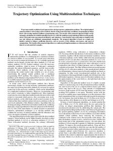
geo-tagged Google Street View images. • 2-D Image/3-D LiDAR Registration: Mastin et al. [15] compare synthetically height color coded 2-D renderings with camera images using Mutual information (MI) [26]. Vasile et al. [25] derive pseudo-intensity images from LiDAR data including shadows to allow for a 2-D/3-D registration with aerial imagery. Feature based approaches [4, 3] mostly rely on the detection and alignment of geometrical features like corners, line segments or planes in the camera image and projections of those from the 3-D data. Figure 1. System overview.
To the best knowledge of the authors there is no literature about multi-modal mapping systems which use large-scale LiDAR data for localization and metric-mapping. In this work we point out important details about incorporating LiDAR data into such a system. We describe our approach for generating LiDAR feature maps. The term feature map refers here to a set of local feature descriptors with attached 3-D coordinates from scanned data. We shed some light on the generation of consistent feature sets by generating normalized synthetic LiDAR intensity images. We further propose to use LiDAR point clouds as a metric multi-modal calibration body for an accurate intrinsic calibration of cameras. The outline of the paper is as follows: first we describe the key components of the system and discuss specific details for using LiDAR scans as an additional information source in monocular mapping systems. We start with details about feature map generation like scan registration, intensity normalization and view generation. Then we describe our method for image based localization, e.g., local correspondence search and camera calibration for multi-modal data. Then we focus on the integration of localized view constraints in a pose graph optimization framework. We evaluate the method with different motion sequences and highly precise terrestrial laserscans of a small city. In the end, we discuss the results and point out further research directions.
2. Method We focus on the representation and integration of LiDAR data in an Image Based Localization and Camera Trajectory Optimization module (red box in Fig.1) since the tracking front-end and state optimization back-end are analog to [22]. The mapping system can be decomposed into the following sub-components: • Tracking Front-End: A local feature approach handles initialization, short term camera tracking and feature track generation. The feature tracks serve as input for the state optimization module.
• State Optimization Back-End: The state optimization back-end is based on a windowed bundle adjustment (BA) framework to simultaneously determine the motion trajectory and mapped 3D-structure. • Multi-Modal Camera Calibration: The calibration module determines the intrinsic camera parameters and distortion coefficients based on LiDAR data. • Loop Detection and Trajectory Optimization: Based on the pose information from the registration framework we use a graph-optimization in combination with a BA framework to correct the mapped structure and camera trajectories. The proposed methodology is as follows: (A) First we pre-process the raw LiDAR point cloud data to generate local feature maps (LiDAR feature DB). This involves the 3-D registration of multiple terrestrial and aerial laser scans. Based on this data a consistent feature map is generated. (B) This feature map then enables an appearance based global localization of single camera images. This is achieved by first selecting feature sub-sets from the map and then registering camera images with a Ransac based 2-D/3-D PnP [11] solver. The registration is then optionally refined by using an intensity based registration. (C) The registered views are used as additional constraints for loop-closures in a pose graph optimization framework to correct the mapped structure and motion of the system.
2.1. Feature-Map Generation (A) Standard terrestrial scanners achieve ranging accuracies of a few millimeters at distances up to 200 hundred meters. Our dataset is based on multiple terrestrial and one aerial LiDAR scan. The whole point cloud consists of approx. 109 data points. In order to handle the visualization and feature generation of the huge datasets we downsample the data using octree datastructures. After the removal of
small scanning artefacts using a statistical outlier filter we generate the feature map using the following procedure:
2.1.1
Scan Preprocessing
To enable a local feature based location recognition system we generate synthetic intensity images from the 3D LiDAR data using a point based rendering. The synthetic views are based on the intensity of backscattered laser pulses. We generate synthetic images around the original laser scanner positions. We only use very small displacements (e.g. 12m) w.r.t. the scanner position to avoid shadowed areas in the synthetic views. However, we densely sample the whole view hemisphere and use a large field of view (e.g., 80 deg) in order to efficiently generate projectively distorted image patches as well. Based on these images we extract features using local image descriptors like Surf [1] or Sift[14]. The 3Dcoordinates of the feature positions are also determined using the GPU-depth buffer information at the feature detector position from the rendered views. All feature descriptors L = {d1 , d2 , ..., dm } around a scanner position are then pooled in a scanner position L feature dataset. Then we compute a KD-Tree and repeat this procedure for all laser scanner positions.
2.1.2
2.1.3
Intensity Normalization
To calculate consistent feature descriptors based on multiple raw LiDAR datasets one must account for varying backscattered laser intensities taken at different positions, angles and distances. Thus we implemented an intensity normalization based on an energy balance and a Lambertian reflection model [8, 5]. In this model the received energy Ir depends on the transmitted energy It , the object surface distance R and the incidence angle θ, which denotes the inclination angle between the surface normal and the laser beam direction. The surface angles are calculated using covariance matrices of local volume cells (comprising of approx. 30 points). The eigenvector of the smallest eigenvalue then served as an approximation for the surface normal (Fig.2). To this end we used the following approximate model equation: 1 (1) Ir = It · Ct · Cr · 2 · e−2αR · cos(θ). R Here, Ct and Cr denote constant terms with respect to the laser transmitter and receiver characteristics. The values were determined on empirical results. The term e−2αR models atmospheric attenuation effects while cos(θ) accounts for the surface orientation. For a more detailed description of LiDAR scan intensity normalization we refer to [5]. Based on the normalized intensity images we calculated the feature descriptors (Fig.2) for the vision based mapping module.
3-D LiDAR Scan Registration
The global localization of a query image with feature maps from multiple raw LiDAR datasets requires a common coordinate system and therefore the registration of the local laserscan coordinate systems. We choose the local coordinate system of a central LiDAR dataset as reference system. We use the extracted local features from the virtual views to automatically find 2-D/2-D appearance based correspondences in rendered views between the scanning positions. After backprojection of the feature locations we finally get 3-D/3-D correspondences for the estimation of a rigid 3D transformation. Based on the correspondences we (RANSAC) estimate the transformation by using Horns method to solve for the least squares approximate solution connecting the local laser scan coordinate systems. For the difficult initial appearance based matching of airborne and terrestrial laserscans we generated Nadir1 views from the terrestrial and aerial datasets. Then we used the recently proposed self-similarity descriptors [21] in combination with a generalized Hough-Transform [2] to find 2D/2-D correspondences based on the intensity information. The initial registration is then further refined using ICP. 1 The knowledge of the Nadir direction w.r.t. the local coordinate systems is assumed to be known for the laserscans.
Figure 2. Local regions: extracted local image regions from the laser scans (top), (bottom) query feature (a) and retrieved point correspondence candidates (b - 1st NN),(c - 2nd NN),(d - 3rd NN). The correct matching feature is (d).
2.2. Appearance Based Global Localization (B) Given the local feature maps in combination with the 3Dinformation from the scanned surfaces we are now able to estimate the 6-DoF pose of given query camera images using an Ransac based PnP solver approach.
2.2.1
Feature Set Selection
An important step in the proposed image based location recognition system is the selection of a sub-set of image features referring to the scanner position L = {d1 , d2 , ..., dm } and the camera query image Q. The images are also modeled as a set of i.i.d. feature descriptors Q = {d1 , d2 , ..., dn }. The selection is achieved by a simple MAP approach with respect to the distribution of image features found in the query and synthetically generated laserscan images around the scanning position L under the assumption of a uniform laserscan prior p(L). ˆ = arg max p(L|Q) = arg max p(Q|L). L L L
(2)
The probabilistic model is based on a generative NaiveBayes approach: P (Q|L) = p(d1 , d2 , ..., dn |L) =
n Y
p(di |L)
(3)
i=1
Using the log probability we arrive at the following decision rule for choosing relevant scanning position feature sub-sets: ˆ = arg max p(L|Q) = arg max 1 L L L n
n X
Intensity Based Pose Refinement
To achieve very high accuracy for registered poses we additionally maximize an intensity based similarity measure between rendered views and the query images. The convergence range of intensity based multi-modal 2D/3D methods is usually very small. The local feature based pose computation usually provides a sufficiently close starting point. An important design choice is the selection of an appropriate distance measure. Mutual Information [26] is considered the gold standard similarity measure for multi-modal matching. It measures the mutual dependence of the underlying image intensity distributions: D(M I) (IR , ITθ ) = H(IR ) + H(ITθ ) − H(IR , ITθ ) (6) where H(IR ) and H(ITθ ) are the marginal entropies and
i=1
m
1 X pˆ(di |L) = K(di − dL j ). m j=1
(5)
with K(·) being a Gaussian kernel, i.e., K(d − dC j ) =
1 L 2 2 exp(− 2σ2 d − dj 2 ) as Parzen kernel function and m the number of features in the synthetic laser-scan images. Due to the Gaussian kernel, descriptors with a high descriptor distance have only a negligible effect. Therefore we approximate the density with the k-nearest (k=2-4) neighbors. However, this leads to small underestimation of the real probability density. Despite its simplicity, the approach is quite efficient and most importantly it allows for a simple update or addition of new feature sets. Since the nearest neighbor relation is not symmetric we adapt the idea of Li and Snavely [12] which establish correspondences from the large database feature set to the small query image feature set. A naive approach, e.g., matching all features from the LiDAR scans with the features of the image, is computationally not feasible (LiDAR feature set size ≥ 107 features). Our approach first searches from the query image feature the k nearest neighbors in the large feature set of the synthetic views and then matches potentially non-negative function which integrates to 1
2.2.2
log p(di |L).
(4) To estimate the descriptor density pˆ(di |L) we use a Parzen likelihood estimation:
2a
corresponding features back to the image feature set. We also considered larger values for k (e.g. 3-6) since many correct correspondences are not the nearest neighbors w.r.t. to the descriptor distance. However, this leads to a challenging match filtering stage.
H(IR , ITθ ) =
X
X
X∈ITθ Y ∈IR
p(X, Y )log(
p(X, Y ) ) (7) p(X)p(Y )
is the joint entropy. p(X, Y ) denotes the joint probability distribution function of the image intensities X, Y in IR and ITθ , and p(X) and p(Y ) are the marginal probability distribution functions. However, MI has usually many local minima near the global optimum. Thus we additionally combined it linearly with a gradient correlation [18] similarity measure for enhancing robustness and accuracy. The intensity based refinement is computationally very expensive (approx. 15-25s per image). To this end we used this step only for the joint determination of extrinsic and intrinsic parameters or distortion coefficients. In this case we jointly registered multiple frames (e.g., 5-10) and optimized the similarity measure w.r.t. all parameters at once assuming constant intrinsic parameters.
2.3. Motion and Structure Optimization (C) Recent progress in SfM methods lead to very powerful algorithms which fully exploit the sparsity structure of the underlying problem [13, 10]. Modern mapping systems like [9, 22] now also use SfM techniques in contrast to state of the art filter based solutions like FASTSlam [23]. These Keyframe BA methods now also work in real-time on modern ’off the shelve’ hardware given reasonable sized keyframe sets (e.g., 20-30 frames).
2.3.1
Keyframe Bundle Adjustment
BA techniques [24] are usually applied to simultaneously determine 3D scene structure and camera motion parameters (SfM) from image data by jointly minimizing the reprojection error of multiple image frames using non-linear least squares techniques. The classical approach is based on a simple measurement model z = f (p, q), e.g., a pinhole projection model with q denoting the structure parameters (e.g., 3D points), ˆ z the image observations ,e.g., the measured projections of the 3D points and p the extrinsic (optionally intrinsic) camera parameters. v(p, q) = f (p, q) − ˆ z denotes the reprojection error. Under the assumption of a known covariance Σzz for image measurements typically a weighted least squares model v(p, q) = vT Σ−1 zz v is minimized. In addition, we used the convex Huber ρ(v(p, q)) cost function [6] which intrinsically handles outliers by a linear penalty only. Since this problem has a rich mathematical structure, there was considerable research to exploit the various occurring sparsity patterns [13, 10]. A typical approach is the marginalization to the usually smaller set of camera parameters using the Schur complement, which is also exploited in our system. 2.3.2
Camera Trajectory Optimization
The camera trajectory optimization is cast as a pose graph optimization problem[17, 22]. This approach encodes the camera trajectory optimization by using relative pose constraints between successive camera positions Ti and Tj : ∆Ti,j = Tj · Ti−1
(8)
As representation for the extrinsic camera parameters we employ the minimal encoding of rigid body transformations SE(3) � � R t T = , with R ∈ SO(n), t ∈ Rn , (9) 0 1 and similarity transforms SIM(3) based on the Lie algebra representation. Here, SO(n) denotes the Lie group of rotation matrices with the matrix multiplication as the group operator. In case of R3 the corresponding Lie algebra se(3) leads to a minimal representation of transformations as 6vectors (ω, ν)T , where ω is the axis angle representation of the rotation R and ν the translation vector with respect to the rotated coordinate system. We also use the framework of [22] and optimize over elements of the Lie group of similarity transforms SIM(3). � � sR t . (10) S= 0 1 In this case the exponential map expSIM (3) and the inverse mapping logSIM (3) are defined similarly to the Lie group
of rigid transformations SE(3) and rotations SO(3). � σ � σ e expSO(3) (ω) W ν expSIM (3) ω = = S. 0 1 ν (11) with W analogous to the well known Rodriguez formula. Given a registered view we add additional constraints which encode the relative position of the registered view and views within the transformation chain. ri,j = logSIM (3) ( c Tj c Ti −1 Ti Tj−1 )
(12)
Here c Tk denote transformations with fixed initial parameters: −1 rn,reg = logSIM (3) ( c Treg c Tn −1 Tn Treg )
(13)
The graph optimization framework now minimizes the sum of quadratic deviations from the original motion constraints including the constraints imposed by registered poses. X E(T1 , T2 , ..., Tn , Treg , ...) = rT (14) i,j ri,j i,j
Intuitively, the optimization procedure corrects camera parameters by spreading the pose constraint residuals over multiple transformations in the transformation chain. After minimization the structure points are mapped back and the similarity transforms are transformed back to rigid transformations by simply changing the translation vector to st. The optimization is carried out using a non-linear least squares optimizer, i.e. Levenberg-Marquardt. However, in practice we can not expect that registered poses Treg are absolutely perfect w.r.t. to the given LiDAR dataset. The registration accuracy and uncertainty depends strongly on the scene/view structure and the number and distribution of feature correspondences. Therefore we use the pose optimized camera trajectories only as a new starting point for a subsequent full BA iteration.
3. Experiments and Results We use ground based (720x576px) and low altitude aerial video streams from an unmanned aerial system. The aerial sequences (1280x720px, 68 deg view angle) were obtained using a MD4-200 Microdrones mini-UAV.
3.1. Evaluation Procedure For evaluation we registered multiple frames of the video sequences to the common laser scan coordinate system and carefully checked the registration results by visual inspection. We also determined the intrinsic parameters of the cameras by using the LiDAR scan as calibration body. In this way we determined the ground truth projection matrices
(extrinsic and intrinsic parameters) for multiple camera images. This allows for an accurate evaluation of local feature correspondences, since we now have knowledge about the underlying scene geometry of the camera images. We used the same evaluation procedure as described in [16] based on ROC curves by varying matching thresholds. The automatic determination of True/False-Positives/Negatives was based on the reprojection error of the 3-D and 2-D local feature coordinates (3.0px inlier threshold). In this way we also determined all possible correct correspondences for the determination of recall values.
3.2. Multi Modal Correspondences We evaluated the performance of multi-modal local feature correspondences with respect to varying system parameters, e.g., the number of synthetic features and feature maps. A small subset of the experimental results is shown in Fig.3a-c. First we measured the multi-modal correspondence performance for query images after feature sub-set selection. Using properly adjusted system parameters we got average recall- and precision values of 23.4% and 20% with an average inlier set size of 50 correct correspondences. This already enables the feature based registration with a reasonable number of Ransac iterations. However, only U-SURF descriptors worked well in case of multimodal image pairs. Rotational invariant feature descriptors (see Fig.3b) showed significantly worse results - which is comprehensible since invariance comes at the price of reduced discriminance.
3.3. Runtime Experiments The implementation (C,C++) is based on various open source software libraries from the computer vision community. However, many parts of our combined software framework are early prototypes and not runtime-optimized so far. Therefore the reported time measurements provide only a rough performance estimate. The test system is equipped with a Core i7-980X CPU with an NVIDIA 580GTX GPU. A typical graph based camera trajectory optimization takes around 64ms for 100 keyframes. A re-optimization BA takes around 7s for 100 keyframes. The windowed BA for 20 keyframes takes around 140ms (min 117ms, max 183ms).
3.4. Trajectory And Structure Optimization To evaluate the accuracy of the trajectory optimization module we measured the distances of reconstructed structure points (BA) compared to densely scanned surfaces. However, the scanned data was acquired at a different time and did not cover the whole visible area of the video data. Thus we only used structure points with distances below a certain threshold ,e.g., ≤ 5m. We calculate the average distances of the SfM structure points w.r.t. nearest neighbors
in the dense point clouds (Fig.5a). We reconstructed the motion and structure of 7 forward motion camera sequences. We initialized the BA optimization framework by registering two frames at the beginning of the motion sequence. The average structure error was 2.56m (max 2.71,min 2.47) for uncorrected sequences and 1.84m (max 1.86, min 1.82) for corrected sequences. The corrected sequences also led to an average increase of 78% for inlying structure points w.r.t the above mentioned distance threshold.
4. Conclusion and Future Work In this work we proposed and implemented a multimodal global localization module for a visual mapping system. While the system also works without prior knowledge - the use of previously acquired metric data greatly improved accuracy. Since the acquired monocular images are registered to a global reference frame we can efficiently compensate for scale drift and prevent error accumulation. This is especially helpful in case of weak camera network structures e.g., long forward motion sequences along the optical axis. The global reference frame also allows multiple, cooperative sensor systems in a straightforward way. We find the approach of using sliding window SFMtechniques [22] in combination with a graph based optimization very intriguing since this methodology efficiently handles the available information and feature constraints. In addition it allows for the straightforward integration of prior scene knowledge. We also assume, that the key advantage of using over-parametrized similarity transformations lies in the appropriate modeling of the occurring drift directions. This helps to effectively explore the search space by the optimization procedure. Nevertheless, the robust and accurate registration of multi-modal image data is still difficult due to fundamental differing object appearances. However, modern mapping systems with a decoupled, real-time tracking front-end and an optimization back-end now allow the integration of such non real-time methods. Future research directions are manifold. Many parameters and properties of the image based location recognition system still remain open. We especially work on the integration of recent findings in metric learning and descriptor optimization in order to scale the system to very large datasets. In addition we will explore a vision based indoor mapping scenario. By registering camera images through windows a stabilization of camera trajectories could be achieved even when there is almost no shared 3D-structure between the mapped area and surrounding 3-D scans.
References [1] H. Bay, A. Ess, T. Tuytelaars, and L. V. Gool. Speeded-up robust features (surf). Computer Vision and Image Understanding, 110:346–359, 2008. 1, 3
(a)
(b)
(c)
Figure 3. ROC curves of LiDAR feature maps/camera images correspondences w.r.t. to varying system parameters. (a) Feature map sizes, e.g. number of simulated images per scan location. (b) Features with and without orientation invariance. (c) Intrinsic parameters (view-angle) of simulated intensity images.
[2] C. Bodensteiner, W. Huebner, K. Juengling, J. Mueller, and M. Arens. Local multi-modal image matching based on selfsimilarity. In Proc. IEEE-ICIP, 2010. 3 [3] M. Ding, K. Lyngbaek, and A. Zakhor. Automatic registration of aerial imagery with untextured 3d lidar models. In CVPR, 2008. 2 [4] C. Frueh, R. Sammon, and A. Zakhor. Automated texture mapping of 3d city models with oblique aerial imagery. In Proc. 2nd Int. Symp. 3D Data Processing, Visualization and Transmission 3DPVT 2004, pages 396–403, 2004. 2 [5] H. Gross, B. Jutzi, and U. Thoennessen. Classification of elevation data based on analytical versus trained feature values to determine object boundaries. In 29. WissenschaftlichTechnische Jahrestagung der DGPF, 2009. 3 [6] R. Hartley and A. Zisserman. Multiple View Geometry in Computer Vision. Cambridge University Press, ISBN: 0521540518, second edition, 2004. 5 [7] A. Irschara, C. Zach, J.-M. Frahm, and H. Bischof. From structure-from-motion point clouds to fast location recognition. In Proc. IEEE Conf. Computer Vision and Pattern Recognition CVPR 2009, pages 2599–2606, 2009. 1 [8] G. Kamerman. Laser Radar, Active Electro-Optical Systems, The Infrared & Electro-Optical Systems Handbook. SPIE Engineering Press, Michigan, 1993. 1, 3 [9] G. Klein and D. Murray. Parallel tracking and mapping for small ar-workspaces. In ISMAR, 2007. 4 [10] K. Konolige. Sparse sparse bundle adjustment. In Proc. BMVC, 2010. 4, 5 [11] V. Lepetit, F. Moreno-Noguer, and P. Fua. Epnp: An accurate o(n) solution to the pnp problem. International Journal of Computer Vision, 81:155–166, 2009. 2 [12] Y. Li, N. Snavely, and D. P. Huttenlocher. Location recognition using prioritized feature matching. In ECCV, 2010. 1, 4 [13] M. Lourakis and A. A. Argyros. Sba: A software package for generic sparse bundle adjustment. ACM Trans. Math. Software, 36:1–30, 2009. 4, 5 [14] D. G. Lowe. Distinctive image features from scale-invariant keypoints. International Journal of Computer Vision, 60(2):91–110, 2004. 1, 3
[15] A. Mastin, J. Kepner, and J. Fisher. Automatic registration of lidar and optical images of urban scenes. In CVPR, 2009. 2 [16] K. Mikolajczyk and C. Schmid. A performance evaluation of local descriptors. IEEE Transactions on Pattern Analysis and Machine Intelligence, 27(10):1615–1630, 2005. 1, 6 [17] E. Olson, J. Leonard, and S. Teller. Fast iterative alignment of pose graphs with poor initial estimates. In Proc. IEEE Int. Conf. Robotics and Automation ICRA 2006, pages 2262– 2269, 2006. 5 [18] G. Penney, J. Weese, J. A. Little, P. Desmedt, D. L. Hill, and D. J. Hawkes. A comparison of similarity measures for use in 2-d-3-d medical image registration. IEEE Transactions on Medical Imaging, 17(4):586–595, 1998. 4 [19] D. Robertson and R. Cipolla. An image based system for urban navigation. In BMVC, 2004. 1 [20] G. Schindler, M. Brown, and R. Szeliski. City-scale location recognition. In Proc. IEEE Conf. Computer Vision and Pattern Recognition CVPR ’07, pages 1–7, 2007. 1 [21] E. Shechtman and M. Irani. Matching local self-similarities across images and videos. In CVPR, 2007. 3 [22] H. Strasdat, J. M. M. Montiel, and A. J. Davison. Scale driftaware large scale monocular slam. In Robotics: Science and Systems, 2010. 1, 2, 4, 5, 6 [23] S. Thrun, W. Burgard, and D. Fox. Probabilistic Robotics. MIT Press, Cambridge, MA, 2005. 1, 4 [24] B. Triggs, P. McLauchlan, R. Hartley, and A. Fitzgibbon. Bundle Adjustment – A Modern Synthesis. Springer-Verlag, 2000. 1, 5 [25] A. Vasile, F. R. Waugh, D. Greisokh, and R. M. Heinrichs. Automatic alignment of color imagery onto 3d laser radar data. In AIPR, 2006. 2 [26] P. Viola and W. Wells. Alignment by maximization of mutual information. International Journal of Computer Vision, 24(2):137–154, 1997. 2, 4 [27] B. Williams, G. Klein, and I. Reid. Real-time slam relocalisation. In ICCV, 2007. 1 [28] A. R. Zamir and M. Shah. Accurate image localization based on google maps street view. In ECCV, 2010. 1
(a)
(b)
(c)
Figure 4. Visualization of the underlying 3D model. Multiple terrestrial scans (a) are jointly registered with an aerial laserscan (b) and serve as the underlying 3D model of the environment. (c) Mixed overlay of a camera image with a synthetic LiDAR intensity image generated with the same intrinsic and extrinsic parameters. The registered images impose constraints on the reconstructed camera trajectory from the mapping system.
(a)
(b)
Figure 5. Visualization of the reconstructed structure (a) and motion (b) of a video sequence superimposed on terrestrial laser scans in a geo-referenced global coordinate system (red cross). The red dots (a) show the reconstructed structure using BA alone (same initialization) while the blue dots show the structure after pose graph optimization. The additional registration constraint lead to a different camera trajectory (red cameras) compared to an approach based on BA alone (blue cameras).
(a)
(b)
Figure 6. Visualization of a registered aerial view from an MD-400 drone camera sequence (a) and the used feature correspondences (b) to compute the registration. The camera image (a) is overlaid with edges extracted from a synthetic view of the laser point-cloud.