2Atmospheric Chemistry Division, National Center for Atmospheric. Research ... St.‐Quentin, CNRS/INSU, Paris, France. Copyright 2011 by ..... Table 1. Total CO Emissions in Tg/yr for Years 2000/2001, 2002, 2003, and 2004a. April 2000 to ...
JOURNAL OF GEOPHYSICAL RESEARCH, VOL. 116, D05304, doi:10.1029/2010JD014416, 2011
Ten years of CO emissions as seen from Measurements of Pollution in the Troposphere (MOPITT) A. Fortems‐Cheiney,1 F. Chevallier,1 I. Pison,1 P. Bousquet,1 S. Szopa,1 M. N. Deeter,2 and C. Clerbaux3 Received 28 April 2010; revised 24 November 2010; accepted 3 January 2011; published 11 March 2011.
[1] The Measurements of Pollution in the Troposphere (MOPITT) retrievals are used as top‐down constraints in an inversion for global CO emissions, for the past 10 years (from March 2000 to December 2009), at 8 day and 3.75° × 2.75° (longitude, latitude) resolution. The method updates a standard prior inventory and yields large increments in terms of annual regional budgets and seasonality. Our validation strategy consists in comparing our posterior‐modeled concentrations with several sets of independent measurements: surface measurements, aircraft, and satellite. The posterior emissions, with a global 10 year average of 1430 TgCO/yr, are 37% higher than the prior ones, built from the EDGAR 3.2 and the GFEDv2 inventories (1038 TgCO/yr on average). In addition, they present some significant seasonal variations in the Northern Hemisphere that are not present in our prior nor in others’ major inventories. Our results also exhibit some large interannual variability due to biomass burning emissions, climate, and socioeconomic factors; CO emissions range from 1504 TgCO (in 2007) to 1318 TgCO (in 2009). Citation: Fortems‐Cheiney, A., F. Chevallier, I. Pison, P. Bousquet, S. Szopa, M. N. Deeter, and C. Clerbaux (2011), Ten years of CO emissions as seen from Measurements of Pollution in the Troposphere (MOPITT), J. Geophys. Res., 116, D05304, doi:10.1029/2010JD014416.
1. Introduction [2] Both as an air pollutant and as a key player in atmospheric chemistry, carbon monoxide (CO) is an active research topic that requires accurate representation of the location and magnitude of CO surface emissions. At northern midlatitudes, CO is mainly emitted by incomplete fossil fuel combustion while biomass burning is its main source in tropics and in the Southern Hemisphere. Given the large spatiotemporal variability of CO emissions, simplifications have to be introduced in order to inventorize them for large regions: the inventories are built using national inventory statistics and emission factors per activity type, and they suffer from large uncertainties [Streets et al., 2006; Klimont and Streets, 2007]. [3] In this context, attempts have been made to deduce CO emissions from CO atmospheric concentrations by statistical inversion methods. The first inversion studies relied on the concentration measurements from the NOAA/ Earth System Research Laboratory (ESRL) surface network [Bergamaschi et al., 2000; Pétron et al., 2002; Kasibhatla et al., 2002]. The operation of the Measure1 Laboratoire des Sciences du Climat et de l’Environnement, CEA‐ CNRS‐UVSQ, Gif‐sur‐Yvette, France. 2 Atmospheric Chemistry Division, National Center for Atmospheric Research, Boulder, Colorado, USA. 3 LATMOS‐IPSL, UPMC Université Paris 06/Université Versailles St.‐Quentin, CNRS/INSU, Paris, France.
Copyright 2011 by the American Geophysical Union. 0148‐0227/11/2010JD014416
ments of Pollution in the Troposphere (MOPITT) instrument on board NASA’s Terra satellite since March 2000 triggered similar studies based on remote sensing data at a global scale [Arellano et al., 2004, 2006; Pétron et al., 2004; Yurganov et al., 2010], at a regional scale [Allen et al., 2004; Heald et al., 2004; Turquety et al., 2008; Tanimoto et al., 2008] or for specific events [Pfister et al., 2005; Turquety et al., 2007]. They were based on the CO retrievals MOPITT Version 3 release and they were restricted to short periods such as 2000–2001 and operated at a subcontinental resolution. The introduction of a variational approach for this kind of study [Stavrakou and Müller, 2006; Henze et al., 2007; Chevallier et al., 2009; Kopacz et al., 2009, 2010] allows more flexibility in the inversion: longer periods can be processed at finer resolution with a larger number of interactive chemical species. [4] The retrieval algorithms that generate the CO profiles from the MOPITT radiance observations have also dramatically improved recently, with enhancements of the general formulation of the retrieval and of its individual components, like the radiative transfer model [Deeter et al., 2010]. The latest version (Version 4) of the retrievals has been released in June 2009. [5] This paper takes advantage of these recent developments and presents the first estimation of the global CO emissions from MOPITT Version 4 data for the decade 2000–2009. It extends the preliminary study of Chevallier et al. [2009] that focused on the African continent for years 2000–2006. Our approach is based on a simplified chemical transport model (CTM), LMDz‐SACS, embedded
D05304
1 of 17
D05304
FORTEMS‐CHEINEY ET AL.: GLOBAL CO EMISSIONS FROM MOPITT
D05304
Figure 1. Schematic of the simplified chemistry mechanism SACS: j1‐3 and k1‐5 are the constants of the reactions or of ensembles of reactions. [OH] and the variables indicated in purple are directly optimized by the data assimilation system. in a variational inversion system. This global CTM explicitly represents the evolution of five interacting chemical tracers in the atmosphere: CO, CH4, HCHO, H2 and methyl chloroform (MCF). OH concentrations link them all together and are constrained by MCF measurements simultaneously. Chemistry of hydrocarbons is also taken into account in this system via a priori computation of the important terms (e.g., secondary CO or HCHO production) using a CTM with more complete chemistry. [6] The components of the inversion system are described in section 2. Section 3 gives the results of the inversion and explores their main features. The inverted emissions are evaluated by comparison of the modeled concentrations with independent measurements at the surface (NOAA/ ESRL, AGAGE, CSIRO, EMPA, SAWS, NIWA and JMA/ MRI), from aircrafts (YAK‐AEROSIB) and from satellite (Infrared Atmospheric Sounding Instrument, IASI). Section 6 focuses on the advantages and limitations of our method.
2. Methodology [7] Our inversion method [Chevallier et al., 2009] aims at adjusting the emissions, jointly called x, in such a way that they become consistent both with the atmospheric observations y and with some prior state xb, given their respective uncertainties represented by their error covariance matrix R and B. The uncertainties are assumed to be Gaussian‐distributed. The solution, which will be called “posterior” in the following, is found by the iterative minimization of a Bayesian cost function J defined as J ðxÞ ¼ ðx � xb ÞT B�1 ðx � xb Þ þ ð H ðxÞ � yÞT R�1 ð H ðxÞ � yÞ: ð1Þ
[8] The vector x contains (1) the global CO, CH4, H2 and methylchloroform MCF emissions at an 8 day and at a
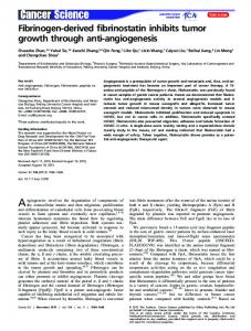
3.75° × 2.75° (longitude, latitude) resolution together with their 3D initial conditions, (2) the factors, at the same resolution, to scale at once the surface emissions and the 3‐D chemical production (by VOCs) of HCHO, and (3) the scaling factors for the 4‐D OH atmospheric concentrations for four latitude bands (90°S–30°S, 30°S–0°, 0°–30°N, 30°N–90°N). The constraints in y are the observations of concentrations of CO and MCF. In this study, CH4, H2 and HCHO are not constrained by dedicated observations. The results of the inversion on these species are very close to the priors. Since CH4, H2 and HCHO are not the species of interest in this study, the results for these species are not shown here. [9] For technical reasons, the 10 year period considered here is processed in consecutive 13 month chunks with a 1 month overlap from one chunk to the next. About 25 iterations are needed to reduce the norm of the gradient of J by 95% with the M1QN3 limited‐memory quasi‐ Newton minimization algorithm that we use [Gilbert and Lemaréchal, 1989]. 2.1. The Chemistry Transport Model [10] The global 3‐D CTM of the atmosphere LMDZ‐ SACS links the variables to the inferred x and the observed variables y. It is derived from the general circulation model LMDZ developed at Laboratoire de Météorologie Dynamique [Hourdin et al., 2006] and of the Simplified Atmospheric Chemistry System (SACS) that has been specifically designed for this inversion system [Pison et al., 2009]. The simplifications of SACS refer to the INCA scheme of Hauglustaine et al. [2004] and Folberth et al. [2006]. As seen in Figure 1, SACS aims to represent the oxidation chain of methane by solving the chemical interaction between a limited set of four species: CO, CH4, HCHO and OH. It is assumed that only the production and the loss of CH4, HCHO, CO and H2 are key for the problematic we
2 of 17
D05304
FORTEMS‐CHEINEY ET AL.: GLOBAL CO EMISSIONS FROM MOPITT
investigate: all other intermediate reactions are considered as instantaneous. [11] The tangent linear and adjoint codes of LMDz‐SACS have been developed by Chevallier et al. [2005] and by Pison et al. [2009]. 2.2. Prior Emissions [12] The prior information xb provided to the inversion system combines two data sets: version 2 of the Global Fire and Emission database GFED‐v2 [Van der Werf et al., 2006] for biomass burning, valid until 2008, and version 3.2 of the Emission Database for Global Atmospheric Research (EDGAR3.2) inventory, valid for 1995, for the anthropogenic emissions (industry, fossil fuel, and industrial biofuel combustion) [Olivier and Berdowski, 2001]. No effort is made here to adapt the 1995 EDGAR3 inventory to the 00’s or the GFED‐v2 data to year 2009 in the prior as the inversion can adjust each pixel of the surface, each week. Emissions and chemistry of other species like the biogenic ones or nonmethane volatile organics compounds (NMVOC) are those described by Folberth et al. [2006] for LMDZ‐INCA; the anthropogenic NMVOC and NOx emissions are estimated as given by the EDGAR v3.2 database, the biogenic NMVOC emissions were taken from the Global Emissions Inventory Activity (GEIA) database [Guenther et al., 1995]. [13] Considering the large uncertainties that still affect such emission inventories, the error standard deviations assigned to the CO prior emissions in the covariance matrix B are arbitrarily set at 100% of the maximum value of the emission time series during the corresponding year for each grid point. This choice of a relatively large value has been made to relax the constraint on the prior emissions. This was found especially important for highly seasonal emissions such as fires [Chevallier et al., 2009]. Errors are set at 100% of the flux for CH4 and H2, and for the HCHO scaling factors. For MCF emissions, the inventory by Montzka et al. [2000] is rescaled according to an update of the study by Bousquet et al. [2005]. As its emissions are supposed to be well known and in order to constrain OH, errors are set at only 1% of the flux for MCF. The errors assigned to the scale factor of OH are set at 10%, which is consistent with the differences between estimates of the OH concentrations of several studies [Prinn et al., 2001; Krol and Lelieveld, 2003; Bousquet et al., 2005]. For the initial conditions, errors are set at 10% for HCHO and MCF and at only 3% for CH4 and 5% for CO. [14] Following Chevallier et al. [2007], spatial correlations are defined by an e‐folding length of 500 km over land (1000 km over sea), without any correlation between land and ocean grid points. Indeed, the recent study by Carouge et al. [2010] shows that the spatial correlations based on more physical properties did not prove to perform better in estimating surface fluxes by inversion than the e‐folding decay approach. We neglect temporal correlations, as the state vector is already aggregated on 8 day basis. 2.3. Methyl Chloroform Observations [15] CO and OH concentrations influence each other to a large extent. The realism of the OH fields is therefore important for the inverse modeling for CO emissions. In the absence of sufficient direct observations of OH, indirect
D05304
information is usually exploited, like that from MCF measurements, since MCF has a simple chemistry with OH and well‐known sources [Prinn et al., 2001; Krol and Lelieveld, 2003; Bousquet et al., 2005]. For the present study, a set of stations that measured MCF nearly continuously for the 2000–2008 period has been selected from the AGAGE and NOAA/ESRL networks available on the World Data Centre for Greenhouse Gases (WDCGG) site at http://gaw.kishou. go.jp/wdcgg/. Note that no MCF data are available at the time of writing for year 2009. In this case, errors of the OH concentrations are set to 0.1%. 2.4. MOPITT V4 Observations [16] The observational constraint on CO emissions comes from Version 4 of the Level 2 product of the MOPITT retrievals (http://www.acd.ucar.edu/mopitt/). The MOPITT instrument has been operated nearly continuously for cloud free spots since March 2000, except during the period from May 2001 until August 2001 when the instrument experienced a cooler failure. The data before and after this failure are different (four channels were lost) with a change in the bias. These two periods have been termed Phase I (from March 2000 to May 2001) and Phase II (August 2001–…). An anomaly also lead to a 2 month lack of data in summer 2009 (from the end of July to October). To date, the MOPITT record is the longest archive of tropospheric CO observations from space. 2.4.1. Data Processing [17] We use the 700 hPa–level CO retrievals that have one of the highest sensitivity to the measured radiances in the troposphere [Deeter et al., 2003] together with their associated averaging kernels (AK). The data selection follows the criteria of the MOPITT data quality statement (http:// www.acd.ucar.edu/mopitt/products.shtml, access: February 2010): data within 25° from the poles have been left out, as the weight of the a priori CO profile in the MOPITT retrievals increases toward the pole. Nighttime data may be biased and are not exploited [Crawford et al., 2004]. We then averaged the retrievals at the 3.75° × 2.5° resolution of LMDz‐SACS at the orbit level, in order to reduce the effect of correlated errors between neighboring observations in the inversion system. As the AK profiles do not vary much within the grid cell, we chose to use the AK profile of the first retrieval when several of them are averaged into a super‐observation. After this screening, about one million “super‐observations” remain in the 13 month inversions. [18] Error correlations between super‐observations can be neglected at the 3.75° × 2.5° resolution used for the inversion [Heald et al., 2004], so that the covariance matrix R of the observation errors is defined as diagonal. Only variances are taken into account. The observation error is the quadratic sum of the measurement error reported in the MOPITT data sets, and of the CTM errors set to 50% of the retrieval values according to Pison et al. [2009]. 2.4.2. Differences Between Version 3 and Version 4 [19] Version 4 has been released in June 2009. As shown by Deeter et al. [2010], it benefits from significant advances in radiative transfer modeling, state vector representation, and a priori statistics compared to Version 3 (V3). The retrieval state vector is represented as the logarithm of the volume mixing ratios. In contrast to the V3 products and their seven standard pressure levels, V4 represents the CO
3 of 17
D05304
FORTEMS‐CHEINEY ET AL.: GLOBAL CO EMISSIONS FROM MOPITT
D05304
bias in Version 4 [Deeter et al., 2010], as in Version 3 [Yurganov et al., 2008; Emmons et al., 2009; Drummond et al., 2009]. This positive bias drifts by about 0.5 ppbv/yr on average at 700 hPa, in Version 4 [Deeter et al., 2010]. It
Figure 2. Mean CO concentrations at 700 hPa, in parts per million, for June 2000 with (a) MOPITT Version 3 and (b) MOPITT Version 4.
profile on a 10‐pressure‐level grid: a floating surface plus nine uniformly spaced levels from 900 to 100 hPa for a better representation of the vertical structure of both the CO a priori profiles and the MOPITT weighting functions. The a priori profile varies for each retrieval, which was not the case for V3. [20] The observed MOPITT V3 (Figure 2a) and MOPITT V4 (Figure 2b) CO concentrations at 700 hPa are displayed in Figure 2 for June 2000. Similar features are seen between the both versions with plumes over Africa and East Asia. However, we can see that the MOPITT V4 concentrations are often smaller than the MOPITT V3 ones. MOPITT V4 has been validated using in situ CO profiles, similarly to previous MOPITT V3 validation studies [Emmons et al., 2004, 2007, 2009]. The retrieval performance has been improved particularly in regions of very high and very low CO concentrations, like over the oceans, where a significant negative bias in clean environments such as the South Pacific Ocean [Emmons et al., 2004] affected the MOPITT V3 retrievals in phase II. As a consequence, the mean bias between our prior modeled concentrations and the MOPITT V4 observations is reduced by about 80% compared to V3. However, the MOPITT retrievals suffer from a time‐varying
Figure 3. Mean CO concentrations, in parts per million, for June 2000 in (a) the MOPITT retrievals for the 700 hPa pressure level, (b) the prior concentrations, and (c) the posterior concentrations. The simulations all take the individual MOPITT averaging kernels corresponding to Figure 3a into account. Abscissa and ordinate report the longitudes and latitudes.
4 of 17
D05304
FORTEMS‐CHEINEY ET AL.: GLOBAL CO EMISSIONS FROM MOPITT
D05304
Figure 4. Partition of the continents into 14 regions.
should be noted that the positive bias drift is not taken into account in our observation error and may bias the inversion estimate. However, as shown later in section 5.3, the consistency of the MOPITT‐based inverted fluxes with the IASI‐based ones shows that the impact of the drift remains small.
3. Concentrations 3.1. Spatial Distribution [21] The month of June 2000 is used as an illustration of the inversion system behavior. The MOPITT retrievals at 700 hPa (Figure 3a), the prior concentrations (Figure 3b) and the posterior CO concentrations (Figure 3c) are displayed in Figure 3. As expected, large discrepancies can be seen between the MOPITT measurements and the prior simulation. In general, the prior underestimates the concentrations. The prior concentrations agree with the MOPITT data rather well in the Southern Hemisphere. In the Northern Hemisphere, an underestimation by about 50% is seen over Canada, South East Asia and over the North Pacific temperate ocean. On the contrary, slight overestimations are observed over the central Africa and South American Temperate regions (60%). Overall, the optimization significantly improves the fit of the simulations to the observations by increasing the emissions. 3.2. Seasonal Cycle [22] As the scale of interest is regional, prior and posterior monthly averaged CO mixing ratios are compared to the MOPITT measurements, for the 14 continental regions shown in Figure 4, in Figure 5. In the Northern Hemisphere, largest concentrations are seen around March and April whereas the peak of the concentrations occurs in September and October in the southern one. CO posterior concentrations for the 10 year period present consistent seasonal cycles in all regions compared to the corresponding prior, even if the amplitude of these cycles can be different. For example, the prior modeled concentrations are lower than
the posterior ones by around 15 ppb over Europe and USA and over the boreal regions in 2008 and 2009. By construction, the optimization brings the model values much closer to the MOPITT measurements. However, as illustrated in Figure 5j with the Indonesian emission peaks in 2002, 2004 and 2006, the model does not exactly fit the observations since the posterior is pulled both toward the observations and toward the prior.
4. Emissions 4.1. Annual and Regional Budget of CO Emissions [23] This section focuses on the results in terms of inverted emissions from March 2000 to December 2009. The results are summarized per year and per region in Table 1, in Table 2, and in Figure 6. [24] As expected [Carmichael et al., 2003; Palmer et al., 2003; Pétron et al., 2004; Arellano et al., 2004; Allen et al., 2004; Heald et al., 2004; Wang et al., 2004; Streets et al., 2006], the inversion highlights the importance of South East Asia as a CO source with an average of 280 TgCO/yr, followed by South American Temperate (154 Tg/yr), Northern Africa (143 Tg/yr), Southern Africa (140 Tg/yr), USA (136 Tg/yr) and Europe (130 Tg/yr). [25] Most of the MOPITT‐based inversions published so far have focused on Phase I. Our inverted total CO surface emissions estimates for this period are presented in Table 1. Our posterior budget of 1386 TgCO/yr is 3% higher than the optimized magnitudes obtained by Arellano et al. [2006] with 1342 TgCO/yr (from April 2000 to April 2001). We also compare our estimate with that of Kopacz et al. [2009], who obtained a global budget of 1148 TgCO, which is 16% higher than our estimate. However, our posterior budget of 1276 TgCO/yr (from May 2000 to April 2001) is lower than estimated by Stavrakou and Müller [2006] with 1333 TgCO/yr. [26] For the months April 2000 to March 2001, our posterior total emissions (1271 TgCO/yr) are also higher than the 1091 TgCO/yr (+16%) of Pétron et al. [2004]. Their
5 of 17
D05304
FORTEMS‐CHEINEY ET AL.: GLOBAL CO EMISSIONS FROM MOPITT
Figure 5. Times series of CO concentrations observed by MOPITT (green) and simulated by the prior (blue) and the posterior (red) concentrations from March 2000 to December 2009. Units are ppm. 6 of 17
D05304
D05304
D05304
FORTEMS‐CHEINEY ET AL.: GLOBAL CO EMISSIONS FROM MOPITT
Table 1. Total CO Emissions in Tg/yr for Years 2000/2001, 2002, 2003, and 2004a April 2000 to March 2001
North Am Boreal USA South Am Trop South Am Temp Northern Africa Southern Africa Western Europe Eastern Europe Eurasian Boreal Middle East South Asia South East Asia Indonesia Australia Globe
2002
2003
2004
Prior
Posterior
Prior
Posterior
Prior
Posterior
Prior
Posterior
5 118 50 51 172 100 72 41 37 24 80 166 39 32 1007
18 116 49 122 155 132 63 39 93 43 47 260 42 74 1271
13 118 36 70 156 99 70 45 55 24 81 165 90 32 1074
45 151 18 150 153 134 77 50 108 101 49 268 62 88 1475
15 116 60 63 141 101 70 38 79 24 80 163 52 32 1053
69 137 44 137 137 132 86 47 144 77 59 249 22 82 1443
21 116 35 116 148 98 69 39 18 24 80 185 71 25 1063
70 129 14 170 149 134 89 48 80 87 60 279 37 80 1441
a
Prior denotes before inversion, and Posterior denotes after inversion. The total estimates include the oceanic CO source amounting to 20 TgCO/yr. All budgets correspond to a 12 month period.
optimized value of 207 TgCO/yr for South East Asia is lower than our estimate of 260 TgCO/yr. There are large discrepancies for regions such as Eurasian Boreal, where we found higher emissions (+348% with 93 TgCO), or Australia, where we found lower emissions (−22% with 74 TgCO). For the south Asian region, Pétron et al. [2004] obtain a 121 TgCO annual total, an increase of 21% relative to their prior emissions. In contrast, Heald et al. [2004] estimate the Indian emissions (corresponding to our South Asian region) to be 46 TgCO/yr, that is 50% lower than their prior of 90 TgCO/yr and equivalent to our posterior estimate of 47 TgCO. [27] Kopacz et al. [2010] recently inverted CO emissions from May 2004 to April 2005, combining CO column measurements from the MOPITT, from the Atmospheric Infrared Sounder (AIRS) and from the SCanning Imaging Absorption SpectroMeter for Atmospheric CartograpHY (SCIAMACHY) satellite. Their total surface emissions constitute 1350 TgCO, 9% lower than our estimate of 1474 TgCO for the same period. Kopacz et al. [2010] estimated the annual emissions in Alaska and Canada to be about 24 TgCO, 20% lower than the summer emissions
estimate (from June to August) of Pfister et al. [2005] and Turquety et al. [2007] and 70% lower than our posterior value of 41 TgCO. The main difference between our two studies is seen for the USA; our value of 127 TgCO disagrees with their posterior emissions of 46.5 TgCO (−164%) and with the study of Hudman et al. [2008]. Hudman et al. [2008] estimated CO emissions over USA to be about 40 Tg and also mentioned that U.S. road emissions are overestimated in the anthropogenic emission inventory from the U.S. Environmental Protection Agency (EPA). The cause of the large difference is unclear. On the one hand, many uncertainties remain in the inventories (e.g., vehicle cold starts [Parrish, 2006]). On the other hand, the transport of the high CO concentrations from the South American Tropical region over USA, may contribute to a misattribution of emissions to the USA in our inversion. [28] One should note that significant differences are observed in any comparison between different global and regional MOPITT‐based inverted results, due to the diversity of the inversion systems (such as the space‐time resolution of the state vector x, the CTM used, whether or not the OH fields are prescribed in the model, the processing of
Table 2. Total CO Emissions in Tg/yr for Years 2005, 2006, 2007, 2008, and 2009 2005
North Am Boreal USA South Am Trop South Am Temp Northern Africa Southern Africa Western Europe Eastern Europe Eurasian Boreal Middle East South Asia South East Asia Indonesia Australia Globe
2006
2007
2008
2009
Prior
Posterior
Prior
Posterior
Prior
Posterior
Prior
Posterior
Prior
Posterior
11 116 36 116 154 107 70 40 18 24 80 168 87 18 1066
63 131 23 184 145 149 82 54 79 75 58 279 49 77 1467
9 117 34 66 141 92 70 41 30 24 80 168 129 29 1047
55 134 19 138 135 133 80 54 89 71 52 286 96 99 1461
7 119 38 121 161 96 70 39 20 24 80 201 44 25 1065
41 124 33 198 166 144 79 44 74 58 57 353 20 92 1504
7 117 36 60 144 104 69 40 41 24 80 164 45 18 969
37 143 27 128 134 146 72 46 99 53 57 250 21 81 1328
7 117 36 60 144 104 69 40 41 24 80 164 45 18 969
26 140 23 131 130 146 79 52 84 48 57 272 28 81 1318
7 of 17
D05304
FORTEMS‐CHEINEY ET AL.: GLOBAL CO EMISSIONS FROM MOPITT
D05304
Figure 6. Total posterior (inverted from MOPITT) CO emissions per year for the 14 regions, in TgCO/yr. the MOPITT V3 or V4 observations). As an example of the CTM diversity, an intercomparison of 26 CTMs showed a wide range of simulated CO distribution, even though the models all used the same emissions for fuel combustion, industry, and biomass burning [Shindell et al., 2006]. 4.2. Error Estimates [29] In principle, the uncertainty of the posterior emissions can be estimated theoretically using the Monte Carlo approach of Chevallier et al. [2007]. However, a simpler estimation method was preferred here because of the large computational expense of the Monte Carlo approach, in particular when the target period for the CO budget extends to a whole year. As a trade off between computing resources and exhaustivity, we simply estimate the inversions one‐ sigma uncertainty from the spread of the regional emissions in five sensitivity tests (cases A to E). [30] 1. In case A, the OH field is replaced by OH‐v2 field, different within 5% from the OH reference. It comes from a simulation of the full chemistry model LMDz‐INCA, using another realistic emission scenario (the combination of anthropogenic emissions from IIASA, QUANTIFY for ship and GFEDv2 for biomass burning). [31] 2. In case B, OH prior concentrations errors set at 35%. [32] 3. In case C, HCHO prior sources increased by 50%. [33] 4. In case D, CO prior emissions error set at 400%. [34] 5. In case E, error correlations length set at 1000 km. [35] The total CO annual emissions for the whole year 2004, found from each test, are given for the 14 regions in Figure 7. These posterior regional results are compared with the reference inversion described in section 2. If the differences between the posterior regional emissions budget as
Figure 7. Annual total posterior CO emissions per region obtained by five sensitivity tests for year 2004 compared to the posterior reference. Case A: OH‐v2 field; Case B: error on the OH concentrations set to 35%; Case C: the HCHO prior sources increased by 50%; Case D: error on the prior CO emissions set to 400%; Case E: error correlations length set to 1000 km. The prior information combines two data sets: EDGAR 3.2 for anthropogenic emissions and GFEDv2 for biomass burning.
8 of 17
D05304
FORTEMS‐CHEINEY ET AL.: GLOBAL CO EMISSIONS FROM MOPITT
Table 3. Regional and Global Error Estimates, as Estimated From Sensitivity Tests for 2004, in Tg/yr Region
Error Estimates
North Am Boreal USA South Am Trop South Am Temp Northern Africa Southern Africa Western Europe Eastern Europe Eurasian Boreal Middle East South Asia South East Asia Indonesia Australia Globe
26 26 6 20 20 8 20 13 22 3 5 33 7 21 166
estimated from this sensitivity study are weak, we assumed that the uncertainty associated with these emissions is small, and conversely. [36] In case A, we investigate the impact of the prior OH field on the inversion; the inversion experiment is carried out with the OH‐v2 field of OH. The impact is small, with differences in yearly emitted masses of a few percent only. In case B, when the OH prior uncertainties were set to 35%, some changes in the estimated regional budgets are observed, in particular over Australia (−20%) and in the Northern Hemisphere (−30% for North American Boreal, −22% for Eurasian Boreal, −20% for Europe and −17% for USA). By relaxing constraints on OH, the MCF observations are able to reduce OH concentrations in the 30°N–90° N latitudinal band, which is counterbalanced with a reduction of the CO emissions in order to keep the fit to the MOPITT retrievals. In case C, the impact of the prior HCHO field is tested by increasing the prior atmospheric source of CO by 50%. The posterior emissions are smaller than in the reference inversion for all regions (−8% for USA, −11% for South American Temperate). When the error on the prior CO emissions is increased to 400% (case D), the posterior yearly emissions are only slightly increased (e.g., for regions South East Asia (+3%) and USA (+2%)). In case E, the impact on the emissions is small (e.g., +2% in USA and −2% in Western Europe). [37] The difference between the regional inverted emissions in cases D and E relative to the reference inversion is small, indicating that the inversion is largely insensitive to the prior errors statistics. The difference is the largest for case C; the HCHO prior field has a strong influence on the posterior CO emissions, even though its impact is limited to less than 15% in the regions that emit more than 100 TgCO/yr. [38] As shown in Table 3, the lowest posterior relative uncertainties are found for the regions: Southern Africa, Middle East, South Asia and South East Asia with uncertainties of 6%, 6%, 9% and 10%, respectively. The uncertainty in regions North American Boreal and South American Tropical reaches 40% and 37.5%, respectively. 4.3. Variations Between Prior and Posterior Emissions [39] Explained by economic developments since 1995 (target year of EDGAR 3.2 inventory), global posterior
D05304
emissions are higher compared to the prior, by about 13% for Phase I and 37% for Phase II (Tables 1 and 2). All regions contribute to this increase of emissions except three of them (South American Tropical, Indonesia and South Asia). The yearly mean emissions are significantly increased by the inversion over Australia (e.g., by up to 175% (+56 TgCO) in 2002 or 220% (+55 TgCO) in 2004), as also seen by Jones et al. [2009], and over boreal regions. [40] Figure 8 shows the time series of the prior and posterior monthly CO emissions in each region. The seasonal variation of the posterior source estimates is close to the prior one in most regions, keeping the same interannual variability, even though the amplitude differs. This is the case for regions Indonesia, South East Asia, Middle East, North American Boreal, Eurasian Boreal, South American Temperate, South American Tropical and Northern Africa. [41] There are, however, some interesting differences in seasonality between prior and posterior cycles. As described by Chevallier et al. [2009] and in agreement with Arellano et al. [2004], Bremer et al. [2004] and Stavrakou and Müller [2006], one of these differences is seen in Southern Africa: instead of peaking in July–August like the prior, the posterior estimates peak 2 months later, in September–October. [42] As in findings by Kopacz et al. [2010], our results present a larger‐than‐expected seasonal variation in CO emissions at northern midlatitudes (for regions South Asia, Middle East and USA). Over USA, the posterior emissions peak late in spring rather than in winter. These maximums present higher amplitude than the prior ones (+7 TgCO in average). This could be explained by the fact that CO emissions from domestic wood burning and from vehicle cold starts are not well treated in the a priori emissions inventories [Miller et al., 2008; Parrish, 2006; Kopacz et al., 2010]. As seen in Figure 8h, the south Asian prior sources are about 7 TgCO per month throughout the years, but the posterior sources range from 2 TgCO/month in summer to 10 TgCO/month in winter. However, it should be reminded that the EDGAR v3.2 data inventory was designed for the year 1995 and has been applied here for years 2000–2009. Since then, Asia has benefitted from an important economic growth and emissions have changed, particularly the contribution of the industry, transport and domestic sectors [Streets et al., 2006; Ohara et al., 2007] and its seasonal cycle may be more similar to that of industrial regions. 4.4. Interannual Variability [43] The 10 year inversion for CO emissions allows for investigating interannual variability (IAV). A slight decrease in the annual Western European emissions is observed since 2003 whereas the emissions of USA and Eastern Europe seem to be constant. However, global CO emissions show significant interannual variability, in particular in tropical and subtropical regions where the interannual variation is mostly influenced by biomass burning [Szopa et al., 2007], and partly by precipitation rates [Van der Werf et al., 2008]. [44] Boreal regions (North American Boreal and Eurasian Boreal) and Indonesia display a notable IAV. For Indonesia, the annual budgets (Tables 1 and 2) show that the 2006 CO emissions are higher than in other years (96 TgCO/yr, compared with 21 to 49 TgCO/yr for 2005 and 2008–2009). This may be linked to the 2006 El Niño–Southern Oscillation
9 of 17
D05304
FORTEMS‐CHEINEY ET AL.: GLOBAL CO EMISSIONS FROM MOPITT
Figure 8. Times series of prior (blue) and posterior (red) CO emissions from March 2000 to December 2009. IASI posterior is in green, from July 2008 to December 2009. Unit is TgCO/month. 10 of 17
D05304
D05304
FORTEMS‐CHEINEY ET AL.: GLOBAL CO EMISSIONS FROM MOPITT
Table 4. Annual and Global Mean of Prior and Posterior OH Concentrations, in 105 mol cm−3
2000–2001 2002 2003 2004 2005 2006 2007 2008 2009
Prior
Posterior
8.93 8.79 8.78 8.32 8.59 8.52 8.98 8.78 8.97
8.57 8.21 8.07 8.79 8.88 8.99 8.36 8.75 8.97
(ENSO) event, which was associated with drought and the greatest rise in wildfire activity in Indonesia since the record‐ breaking 1997–1998 El Niño [Logan et al., 2008; Chandra et al., 2009]. [45] Global CO emissions range from 1504 TgCO, in 2007, to 1318 TgCO in 2009 (Table 2). Indeed, global CO emissions decreased significantly in 2008 and 2009. These low emissions are considered anomalous by Yurganov et al. [2010], who hypothesized that economic recession could have impacted the CO emissions. From Table 2, it can be seen that only two regions are responsible of this diminution: South East Asia and South American Temperate (−103 TgCO and −70 TgCO, respectively, between 2007 and 2008). For South East Asia, it should be noted that the 2007 biomass burning emissions (particularly the peak in March) were extremely high compared to the other years (e.g., 153, 150, 189, 152 TgCO in GFEDv2 for 2005, 2006, 2007 and 2008), whereas the biomass burning emissions in 2008 could be considered as normal. [46] Significant IAV in CO emissions was observed in the South American Temperate region since 2000 (137, 170, 184, 138, 198, 128, and 131 TgCO/yr for 2003, 2004, 2005, 2006, 2007, 2008 and 2009). This IAV is well correlated (correlation coefficient of 0.90, using 60 monthly values) with the fire counts of Torres et al. [2010] derived from Aqua‐MODIS observations [Giglio et al., 2006], but not with the deforestation rates provided by the Brazilian government remote sensing agency INPE (Instituto Nacional de Pesquisas Espaciais, http://www. obt.inpe.br/prodes/prodes_1988_2009.htm, access: August 2010) (correlation coefficient of 0.44, based on 9 annual values). This apparent inconsistency can be explained by the fact that in this region, biomass burning is the result of the cropland expansion, (and consequently to deforestation [Morton et al., 2006]), but also to other practices, such as the disposal of agricultural waste. [47] After low value in 2006 related to unfavorable climate conditions [Gloudemans et al., 2009; Schroeder et al., 2009], there was a peak in CO emissions in 2007, correlated with the largest number of fires detected from space over the last 10 years [Torres et al., 2010]. In 2008, the decrease in South American emissions cannot be explained by climate conditions [Torres et al., 2010], but may be related to socioeconomic factors connected to the economic recession (with unfavorable market conditions for agricultural exports), such as the soybean price collapse in summer 2008.
D05304
[48] Although the emissions of the two regions South East Asia and South American Temperate slightly increased from 2008 to 2009 (from 250 to 272 Tg and from 128 to 131 Tg, respectively), global CO emissions still decreased in 2009. Except over Europe, all the Northern Hemisphere regions have lower emissions in 2009 than in 2008. This could be due to lower fossil fuel emissions owing to the economic recession. More extensive work is needed to resolve this issue. 4.5. CO Atmospheric Production and Loss [49] Although surface emissions are dominant, CO chemical production and loss can play a role in long‐term changes in the tropospheric chemical composition and they are optimized in the system. The chemical loss of CO corresponds to CO2 production according to the reaction with hydroxyl radical OH: CO + OH → CO2 + H. As mentioned in section 2, OH is constrained by the MCF measurements and optimized in the inversion. The yearly averages of the prior and posterior tropospheric OH concentrations are given in Table 4. For the past 10 years, the global OH posterior concentrations value is 8.62 × 10⁵ mol cm−3 on average, 17% lower than the 10.5 × 10⁵ mol cm−3 value of Prinn et al. [2005]. The posterior total masses of OH vary between −8% (2003) and 6% (2006) of the prior. These variations are within the expected range of OH interannual variability obtained by other inversion studies [Bousquet et al., 2005; Prinn et al., 2005]. [50] Figure 9 shows five examples of the temporal variations of the chemical production and of the chemical loss of CO over the sea (tropical Pacific Ocean and Indian tropical ocean) and over the continent (Northern Africa, USA, Europe). Prior and posterior CO productions are nearly similar, due to the weak impact of the inversion on HCHO concentrations (not shown). Note that the HCHO prior concentrations used here are smaller than the SCIAMACHY retrievals shown by De Smedt et al. [2008, Figures 13 and 14] and present less variability. The production of CO2 is large over tropical regions and particularly over tropical oceans which represent about 30% of the global tropospheric CO2 production. The global CO2 production from 2000 to 2009 ranges from 1120 TgC/yr to 1072 TgC/yr, with a global average of 1118 TgC/yr, 2% smaller than the Folberth et al. [2005] value of 1137 TgC/yr.
5. Evaluation With Independent Measurements [51] Our evaluation strategy consists of comparing our posterior‐modeled concentrations with several sets of independent measurements at the surface, from aircraft, from other inventories and by satellite. 5.1. Comparison With Surface and Aircraft Measurements [52] The posterior emissions are evaluated by comparison of the prior and of the posterior modeled CO concentrations with independent and fixed surface measurements from various networks (NOAA/ESRL, AGAGE, CSIRO, EMPA, SAWS, NIWA and JMA/MRI) available on the WDCGG Web site. We have restricted our analysis to 56 sites that present uninterrupted measurements for the 2000–2008
11 of 17
D05304
FORTEMS‐CHEINEY ET AL.: GLOBAL CO EMISSIONS FROM MOPITT
D05304
Figure 9. Prior and posterior production and loss of CO from March 2000 to December 2009. The loss of CO corresponds to the production of CO2. Note that the scale is different between continental regions (USA, Europe, and Northern Africa) and oceanic regions.
period and, at least, one measure per month. The site locations and results are shown in Figure 10. Stations highlighted in green, for which the ratio of the posterior to the prior bias or root mean square (RMS) is lower than 1, indicate an improvement of the corresponding statistical indicator after optimization. Two different periods are studied here: MOPITT Phase I (March 2000 to May 2001) and Phase II (August 2001–…). [53] During Phase I, the absolute biases are reduced by 2% to 154% at 38 stations. The inversion leads to a dramatic improvement relative to the prior simulation for all the high‐ latitude sites of the Southern Hemisphere (TDF, CRZ, PSA, HBA, SYO, MAA, MQA, CYA, ARH) and for 76% of the stations in the Northern Hemisphere. This percentage then
reaches 84% for Phase II (average ratio for the bias of 0.78), with best results at European stations (PAY, HUN, BSC). [54] However, in Phase II, the inversion degrades the fit for the NOAA POC boats in the South Pacific Ocean. As shown in Figures 10b and 10d, the ratios of bias and RMS of this station are higher than 1 below the equator. The fit is also degraded at the high‐latitude Southern Hemisphere sites, with an average ratio for the bias of 5.22. This feature was already pointed by Arellano et al. [2004] and by Stavrakou and Müller [2006]. [55] We use the airborne campaigns YAK‐AEROSIB carried out in April 2006, August 2007 and July 2008 across Siberia by Paris et al. [2008, 2009, 2010] as an additional independent set of measurements for this region not covered
12 of 17
D05304
FORTEMS‐CHEINEY ET AL.: GLOBAL CO EMISSIONS FROM MOPITT
D05304
Figure 10. (a, b) Ratio of the posterior to the prior values of bias (in absolute value) between simulated and observed concentrations at the 56 surface CO stations for MOPITT Phase I and MOPITT Phase II. (c, d) Same as Figures 10a and 10b but for root mean square (RMS). NOAA/ESRL POC course in the South Pacific Ocean from year 2002 to 2007 and YAK course in Siberia from year 2006 to 2008 are represented by triangles in Figures 10b and 10d. The inversion improved the simulation when the ratio of the absolute bias or RMS is less than 1 (in green). The statistics refer to the differences between the simulated and the observed concentrations of CO.
by the various networks. The inversion improves the fit at the highest latitudes in Siberia with a reduction by 23% of the absolute bias but degrades it about latitude 50°N (Figures 10b and 10d). As for the fixed station UTA, along the western coast of USA, note that there is little or no MOPITT data in this region (as seen in Figure 2), so that it is only constrained indirectly by data over neighboring regions. 5.2. Comparison With Other Inventories [56] Large discrepancies exist between different inventories in terms of budgets [Butler et al., 2008] and in terms of seasonal variability, explained by the respective methodologies used in the inventory construction and by the emission factors applied. We compare our posterior western European, American and Asian emissions with several global and regional inventories that correspond to year 2000: (1) the one proposed for the IPCC fifth assessment report AR5 [Lamarque et al., 2010]; (2) the REanalysis of
the TROpospheric chemical composition (RETRO) inventory [Pulles et al., 2007], developed by The Netherlands Organisation for Applied Research (TNO) (3) the Cooperative Programme for Monitoring and Evaluation of the Long‐range Transmission of Air Pollutants (EMEP) inventory for Europe; (4) the U.S. Environmental Protection Agency (EPA) inventory for USA; and (5) the inventory of Streets et al. [2006] for Asia. [57] As seen in Figure 11a, these inventories show very similar seasonal cycles for Western Europe and our posterior is in good agreement with IPCC AR5 and EMEP. However, as described in the section 4.3, our posterior cycle shows a strong seasonal variation with large intensities in April for USA and the region South East Asia, which is not seen in the others inventories. [58] We have seen that south Asian emissions are still misunderstood and several studies contradict each other about total budgets. It is also the case for the seasonal cycle (Figure 11c). Our posterior emissions for this region show
13 of 17
D05304
FORTEMS‐CHEINEY ET AL.: GLOBAL CO EMISSIONS FROM MOPITT
D05304
Figure 11. Seasonal cycles of different inventories. The anthropogenic emissions are given by the inventories EDGAR 3.2, RETRO, IPCC AR5, EMEP for Europe, EPA for the USA and Streets et al. [2006] for Asia for year 2000. Biomass burning from GFEDv2 has been added to all inventories for comparison with the inverted emissions. Our posterior emissions begin in March 2000. Note that the scale is different for South East Asia. stronger seasonality whereas the IPCC AR5, EDGAR 3.2 and Streets et al. [2006] inventories do not have any seasonality, the emissions are constant among the year but with different levels: 8 TgCO, 6 TgCO and 5 TgCO, respectively. RETRO presents a strongly different cycle with maximum in winter and minimum in July. For South East Asia, all the inventories are similar, except in spring: our posterior and RETRO peak in April instead of March for the others inventories. 5.3. Comparison With a IASI‐Based Inversion [59] The IASI instrument has been flying as part of the METOP‐A platform since October 2006. It provides CO partial columns information [Clerbaux et al., 2009]. Products have been made available by the Laboratoire Atmosphères, Milieux, Observations Spatiales (LATMOS) through the Ether database (http://ether.ipsl.jussieu.fr), for the period starting in June 2008. The retrieval code based on the Optimal Estimation was developed at the Université Libre de Bruxelles [Turquety et al., 2009] and CO data were evaluated against other satellite observations [George et al., 2009]. [60] In a previous study [Fortems‐Cheiney et al., 2009], we have obtained similar global CO emissions budgets from IASI and from MOPITT V3, 643 TgCO and 649 TgCO,
respectively, from July to November 2008. Consistent with this results, the mass budgets for a 1 year period (from July 2008 to June 2009) are also in good agreement. The global IASI posterior emissions of 1450 TgCO are 10% higher than the MOPITT ones (1304 TgCO). It is mostly due to a 331% (+63 TgCO) and 53% (+80 TgCO) increase of the annual fluxes over regions Indonesia and Northern Africa, respectively, with the IASI inversion, which posterior values of 82 TgCO and 230 TgCO are substantially higher than the MOPITT‐based estimate. On the contrary, we notice that the IASI‐based emissions in the Southern Hemisphere are lower than the MOPITT ones, in particular in Australia (−43%). For others regions like Western Europe, USA and South East Asia, both the IASI and MOPITT inversions lead to a similar budget (with 70 and 68 TgCO, 110 and 96 TgCO, and 285 and 292 TgCO, respectively). [61] We compare the impact of the satellite observations on seasonal and regional cycles from July 2008 to December 2009 in Figure 8. The IASI‐based posterior emissions also show a strong seasonality in the Northern Hemisphere. Differences are in some cases noticeable like over Western Europe, Middle East and Australia. The IASI posterior emissions also present higher amplitudes over South Asia (Figure 8h) and Indonesia (Figure 8j) than the MOPITT
14 of 17
D05304
FORTEMS‐CHEINEY ET AL.: GLOBAL CO EMISSIONS FROM MOPITT
ones. However, for the others regions, the MOPITT and IASI posteriors present similar cycles (Northern Africa, North American Boreal, South American Tropical, Eastern Europe, South American Temperate, Southern Africa, Eurasian Boreal and South East Asia). This result is all the more encouraging given the known drift of the MOPITT retrievals discussed by Deeter et al. [2010].
6. Conclusions [62] The inverse modeling approach offers an attractive solution to the problem of estimating the gaseous emissions, that allows one to correct the prior inventories. For the first time, this study aims at estimating the CO emissions for the past 10 years, using a multispecies inversion system and the MOPITT Version 4 retrievals. The “COLSCE‐V1” global gridded CO fluxes, at an 8 day and 3.75° × 2.75° resolution, will be available from the CarboScope Web site: http:// www.carboscope.eu. Our study indicates that the absolute accuracy of the inverted CO emissions at yearly subcontinental scale should be better than 15% in regions that emit more than 100 TgCO/yr. [63] Significant modifications of the prior emissions are seen in our study. First, our posterior emissions differ from the prior ones in terms of budget. The global estimate is higher by about 13% compared to the prior for Phase I (March 2000 to May 2001) of the MOPITT acquisition. For Phase II (August 2001–…), this increase reaches about 37%, explained by the fact that the magnitude of the anthropogenic CO emissions have changed since 1995, target year of EDGAR v3.2, which is our prior. [64] Second, the CO emissions also have some significant interannual variability due to biomass burning emissions, climate, and socioeconomic factors, which requires to be considered for CO modeling. The highest annual budget of the last decade is seen for year 2007 with 1504 TgCO/yr, because of fires over South East Asia and South American Temperate. Then, the CO emissions show a dramatic decrease (1318 TgCO/yr in 2009), that could be connected to the economic recession. [65] The uncertainty on these emissions ranges from 6% (over regions Southern Africa and Middle East) to 40% over the region North American Boreal. In the case of high latitudes, the inverted emissions improve the fit to the northern sites (i.e., BRW, ALT and CBA with absolute bias reduced by 69%, 69% and 54%, respectively) in spite of their relatively large uncertainties. Indeed, a comparison of our posterior‐modeled concentrations to the independent surface measurements shows improved agreement in the Southern Hemisphere and for 76% of the stations in the Northern Hemisphere for Phase I. This percentage then reaches 84% for Phase II. However, in Phase II, the inversion fails to improve both the fit to the YAK‐AEROSIB measurements about latitude 50°N in Siberia, and the fit to the stations located in the high latitudes of the Southern Hemisphere (with an average ratio for the bias of 2.61) and in Australia (stations CFA, CGO). [66] Third, as found by Kopacz et al. [2010], some significant seasonal variations of the emissions in the midlatitudes of the Northern Hemisphere are found with both the MOPITT‐based and the IASI‐based inversions, whereas most anthropogenic inventories do not include any one.
D05304
[67] The consistency of the MOPITT‐based inverted fluxes with the IASI‐based ones shows that the impact of the drift in the MOPITT retrievals does not exclude the possibility of a multidecadal CO monitoring (with the METOP series: METOP‐B in 2012, METOP‐C in 2016). Nevertheless, an alternative to MCF as a constraint for the OH fields has to be found in the near future, as MCF concentrations are declining rapidly (current values are of only a few parts per trillion) to the extent that MCF soon cannot be used to inform about OH anymore. An alternative to MCF could be the use of 14CO [Krol et al., 2008]. Moreover, together with OH, formaldehyde controls the atmospheric production of CO. Ideally, its concentrations should also be constrained in the inversion. Further, our sensitivity tests highlight HCHO prior fields as the less reliable component in our inversion system. Some improvement is therefore expected by integrating HCHO retrievals from SCIAMACHY or from the Ozone Monitoring Instrument (OMI) [Levelt et al., 2006] in the system. [68] Acknowledgments. We acknowledge the NCAR MOPITT and NOAA CMDL Carbon Cycle groups for providing CO measurements. The IASI L1 data are received through the EUMETCast near real time data distribution service. We also acknowledge the ULB IASI group in Brussels (D. Hurtmans and P. Coheur) for developing the FORLI IASI‐ CO retrieval code, the LATMOS IASI team for providing the expertise on how to use the data, and the Ether French atmospheric database (http://ether.ipsl.jussieu.fr) for distributing the IASI data. The French scientists are grateful to CNES for scientific collaboration and financial support. J. D. Paris (LSCE) and P. Nédélec (Laboratoire d’Aérologie) made the YAK‐AEROSIB data available to us. We thank R. Martin and A. van Donkelaar (Dalhousie University) for providing the EMEP and EPA data and D. Streets (Argonne National Laboratory) for his Asian inventory. We contacted all data PIs and in particular thank E. Brunke (SAWS), B. Buchmann (EMPA), D. Cunnold (AGAGE), J. W. Elkins (NOAA), A. Gomez (NIWA), P. Krummel (CSIRO), R. Langenfeld (CSIRO), K. Masarie (NOAA), S. A. Montzka (NOAA), P. C. Novelli (NOAA), T. Seitz (EMPA), P. Steel (CSIRO), and K. Tsuboi (JMA). The authors are grateful to R. L. Thompson (LSCE), to V. Bellassen (CDC Climat), and to three anonymous reviewers for their comments that greatly improved this paper. Finally, we wish to thank F. Marabelle (LSCE) and his team for computer support.
References Allen, D., K. Pickering, and M. Fox‐Rabinovitz (2004), Evaluation of pollutant outflow and CO sources during TRACE‐P using model‐calculated, aircraft‐based, and Measurements of Pollution in the Troposphere (MOPITT)‐derived CO concentrations, J. Geophys. Res., 109, D15S03, doi:10.1029/2003JD004250. Arellano, A., P. Kasibhatla, L. Giglio, G. Van der Werf, and J. Randerson (2004), Top‐down estimates of global CO using MOPITT measurements, Geophys. Res. Lett., 31, L01104, doi:10.1029/2003GL018609. Arellano, A., P. Kasibhalta, L. Giglio, G. Van der Werf, J. Randerson, and G. Collatz (2006), Time‐dependent inversion estimates of global biomass burning CO emissions using Measurement of Pollution in the Troposphere (MOPITT) measurements, J. Geophys. Res., 111, D09303, doi:10.1029/2005JD006613. Bergamaschi, P., R. Hein, C. Brenninkmeijer, and P. Crutzen (2000), Inverse modeling of the global CO cycle: 1. Inversion of CO mixing ratios, J. Geophys. Res., 105, 1909–1927. Bousquet, P., D. Hauglustaine, P. Peylin, C. Carouge, and P. Ciais (2005), Two decades of OH variability as inferred by an inversion of atmospheric transport and chemistry of methyl chloroform, Atmos. Chem. Phys., 5, 2635–2656. Bremer, H., J. Kar, J. Drummond, F. Nichitu, and J. Warner (2004), Spatial and temporal variation of MOPITT CO in Africa and South America: A comparison with SHADOZ ozone and MODIS aerosol, J. Geophys. Res., 109, D12304, doi:10.1029/2003JD004234. Butler, T., M. Lawrence, B. Gurjar, J. van Aardenne, M. Schultz, and J. Lelieveld (2008), The representation of emissions from megacities in global emission inventories, Atmos. Environ., 42, 703–719.
15 of 17
D05304
FORTEMS‐CHEINEY ET AL.: GLOBAL CO EMISSIONS FROM MOPITT
Carmichael, G., Y. Tang, G. Kurata, I. Uno, and D. Streets (2003), Evaluating regional emissions estimates using the TRACE‐P observations, J. Geophys. Res., 108(D21), 8810, doi:10.1029/2002JD003116. Carouge, C., P. Bousquet, P. Peylin, P. J. Rayner, and P. Ciais (2010), What can we learn from European continuous atmospheric CO2 measurements to quantify regional fluxes: Part 1. Potential of the 2001 network, Atmos. Chem. Phys., 10, 3107–3117. Chandra, S., J. R. Ziemkel, B. N. Duncan, T. L. Dielh, N. J. Livesey, and L. Froidevaux (2009), Effects of the 2006 El Niño on tropospheric ozone and carbon monoxide: Implications for dynamics and biomass burning, Atmos. Chem. Phys., 9, 4239–4249. Chevallier, F., M. Fisher, P. Peylin, S. Serrar, P. Bousquet, F.‐M. Breon, A. Chedin, and P. Ciais (2005), Inferring CO2 sources and sinks from satellite observations: Method and application to TOVS data, J. Geophys. Res., 110, D24309, doi:10.1029/2005JD006390. Chevallier, F., F.‐M. Breon, and P. Rayner (2007), The contribution of the Orbiting Carbon Observatory to the estimation of CO2 sources and sinks: Theoretical study in a variational data assimilation framework, J. Geophys. Res., 112, D09307, doi:10.1029/2006JD007375. Chevallier, F., A. Fortems, P. Bousquet, I. Pison, S. Szopa, M. Devaux, and D. Hauglustaine (2009), African CO emissions between years 2000 to 2006 as estimated from MOPITT observations, Biogeosciences, 6, 103–111. Clerbaux, C., et al. (2009), Monitoring of atmospheric composition using the thermal infrared IASI/METOP sounder, Atmos. Chem. Phys., 9, 6041–6054. Crawford, J., et al. (2004), Relationship between measurements of MOPITT and in situ observations of CO based on a large‐scale feature sampled during TRACE‐P, J. Geophys. Res., 109, D15S04, doi:10.1029/ 2003JD004308. Deeter, M., et al. (2003), Operational carbon monoxide retrieval algorithm and selected results from the MOPITT instrument, J. Geophys. Res., 108(D14), 4399, doi:10.1029/2002JD003186. Deeter, M., et al. (2010), The MOPITT version 4 CO product: Algorithm enhancements, validation, and long‐term stability, J. Geophys. Res., 115, D07306, doi:10.1029/2009JD013005. De Smedt, I., J.‐F. Müller, T. Stavrakou, R. van der A, H. Eskes, and M. Van Roozendael (2008), Twelve years of global observation of formaldehyde in the troposphere using GOME and SCIAMACHY sensors, Atmos. Chem. Phys., 8, 4947–4963. Drummond, J., J. Zou, F. Nichitiu, J. Kar, R. Deschambaut, and J. Hackett (2009), A review of 9‐year performance and operation of the MOPITT instrument, Adv. Space Res., 45, 760–774, doi:10.1016/j.asr.2009.11.019. Emmons, L. K., et al. (2004), Validation of measurements of Measurements of Pollution in the Troposphere (MOPITT) CO retrievals with aircraft in situ profiles, J. Geophys. Res., 109, D03309, doi:10.1029/ 2003JD004101. Emmons, L., G. Pfister, D. Edwards, J. Gille, G. Sachse, D. Blake, S. Wofsy, C. Gerbig, D. Matross, and P. Nédélec (2007), MOPITT validation exercises during summer 2004 field campaigns over North America, J. Geophys. Res., 112, D12S02, doi:10.1029/2006JD007833. Emmons, L., D. Edwards, M. Deeter, J. Gille, T. Campos, P. Nédélec, P. Novelli, and G. Sachse (2009), Measurements of Pollution In The Troposphere (MOPITT) validation through 2006, Atmos. Chem. Phys., 9, 1795–1803. Folberth, G., D. Hauglustaine, P. Ciais, and J. Lathière (2005), On the role of atmospheric chemistry in the global CO2 budget, Geophys. Res. Lett., 32, L08801, doi:10.1029/2004GL021812. Folberth, G. A., D. A. Hauglustaine, J. Lathière, and F. Brocheton (2006), Interactive chemistry in the Laboratoire de Meteorologie Dynamique general circulation model: Model description and impact analysis of biogenic hydrocarbons on tropospheric chemistry, Atmos. Chem. Phys., 6, 2273–2319. Fortems‐Cheiney, A., F. Chevallier, I. Pison, P. Bousquet, C. Carouge, C. Clerbaux, P.‐F. Coheur, M. George, D. Hurtmans, and S. Szopa (2009), On the capability of IASI measurements to inform about CO surface emission, Atmos. Chem. Phys., 9, 8735–8743. George, M., C. Clerbaux, P.‐F. Coheur, J. Hadji‐Lazaro, D. Edwards, H. Worden, M. Luo, C. Rinsland, and C. Barnet (2009), Carbon monoxide distributions from the IASI/METOP mission: Evaluation with other spaceborne remote sensors, Atmos. Chem. Phys., 9, 8317–8330. Giglio, L., I. Csiszar, and C. O. Justice (2006), Global distribution and seasonality of active fires as observed with the Terra and Aqua Moderate Resolution Imaging Spectroradiometer (MODIS) sensors, J. Geophys. Res., 111, G02016, doi:10.1029/2005JG000142. Gilbert, J., and C. Lemaréchal (1989), Some numerical experiments with variable‐storage quasi‐Newton algorithms, Math. Program., 45, 407–435. Gloudemans, A. M. S., A. T. J. de Laat, H. Schrijver, I. Aben, J. F. Meirink, and G. R. van der Werf (2009), SCIAMACHY CO over land
D05304
and oceans: 2003–2007 interannual variability, Atmos. Chem. Phys., 9, 3799–3813. Guenther, A., et al. (1995), A global model of natural volatile organic compound emissions, J. Geophys. Res., 100, 8873–8892. Hauglustaine, D. A., F. Hourdin, L. Jourdain, M.‐A. Filiberti, S. Walters, J.‐F. Lamarque, and E. Holland (2004), Interactive chemistry in the Laboratoire de Météorologie Dynamique general circulation model: Description and background tropospheric chemistry evaluation, J. Geophys. Res., 109, D04314, doi:10.1029/2003JD003957. Heald, C., D. Jacob, D. Jones, P. Palmer, J. Logan, D. Streets, G. Sachse, J. Gille, R. Hoffman, and T. Nehrkorn (2004), Comparative inverse analysis of satellite (MOPITT) and aircraft (TRACE‐P) observations to estimates Asian sources of carbon monoxide, J. Geophys. Res., 109, D23306, doi:10.1029/2004JD005185. Henze, D. K., A. Kakami, and J. H. Seinfeld (2007), Development of the adjoint of GEOS‐Chem, Atmos. Chem. Phys., 7, 2413–2433. Hourdin, F., I. Musat, S. Bony, P. Braconnot, and F. Codron (2006), The LMDZ4 general circulation model: Climate performance and sensitivity to parametrized physics with empahsis on tropical convection, Clim. Dyn., 27, 787–813, doi:10.1007/s00382-006-0158-0. Hudman, R. C., L. T. Murray, D. J. Jacob, D. B. Millet, S. Turquety, S. Wu, D. R. Blake, A. H. Goldstein, J. Holloway, and G. W. Sachse (2008), Biogenic versus anthropogenic sources of CO in the United States, Geophys. Res. Lett., 35, L04801, doi:10.1029/2007GL032393. Jones, D., K. Bowman, J. Logan, C. Heald, J. Liu, M. Luo, J. Worden, and J. Drummond (2009), The zonal structure of tropical O3 and CO as observed by the Tropospheric Emission Spectrometer in November 2004 ‐ Part 1: Inverse modeling of CO emissions, Atmos. Chem. Phys., 9, 3547–3562. Kasibhatla, P., J. Logan, P. Palmer, and P. Novelli (2002), Top‐down estimate of a large sources of atmopsheric carbon monoxide associated with fuel combustion in Asia, Geophys. Res. Lett., 29(19), 1900, doi:10.1029/ 2002GL015581. Klimont, Z., and D. Streets (2007), Emissions inventories and projections for assessing hemispheric or intercontinental transport, in Hemispheric Transport of Air Pollution 2007, Atmos. Pollut. Stud., vol. 16, edited by T. Keatin and A. Zuber, U. N., Geneva, Switzerland. Kopacz, M., D. J. Jacob, D. K. Henze, C. L. Heald, D. G. Streets, and Q. Zhang (2009), Comparison of adjoint and analytical Bayesian inversion methods for constraining Asian sources of carbon monoxide using satellite (MOPITT) measurements of CO columns, J. Geophys. Res., 114, D04305, doi:10.1029/2007JD009264. Kopacz, M., et al. (2010), Global estimates of CO sources with high resolution by adjoint inversion of multiple satellite datasets (MOPITT, AIRS, SCIMACHY, TES), Atmos. Chem. Phys., 10, 855–876. Krol, M., and J. Lelieveld (2003), Can the variability in tropospheric OH be deduced from measurements of 1,1,1‐trichloroethane (methyl chloroform)?, J. Geophys. Res., 108(D3), 4125, doi:10.1029/2002JD002423. Krol, M., J. Meirink, P. Bergamashi, J. Mak, D. Lowe, P. Jockel, S. Houweling, and T. Rockmann (2008), What can 14CO measurements tell us about OH?, Atmos. Chem. Phys., 8, 5033–5044. Lamarque, J.‐F., et al. (2010), Historical (1850–2000) gridded anthropogenic and biomass burning emissions of reactive gases and aerosols: Metholody and application, Atmos. Chem. Phys., 10, 7017–7039. Levelt, P., E. Hilsenrath, G. Leppelmeier, G. van den Oord, P. Bhartia, J. Tamminen, J. de Haan, and J. Veefkinf (2006), Science objectives of the Ozone Monitoring Instrument, IEEE Trans. Geosci. Remote Sens., 44, 1199–1208. Logan, J. A., I. Megretskaia, and R. Nassar (2008), Effects of the 2006 El Nińo on tropospheric composition as revealed by data from the Tropospheric Emission Spectrometer (TES), Geophys. Res. Lett., 35, L03816, doi:10.1029/2007GL031698. Miller, S., et al. (2008), Sources of carbon monoxide and formaldehyde in North America determined from high‐resolution atmospheric data, Atmos. Chem. Phys., 8, 7673–7696. Montzka, S., C. Spivakosky, J. Butler, J. Elkins, L. Lock, and D. Mondeel (2000), New observational constraints for atmospheric hydroxyl on global and hemispheric scales, Science, 288, 500–503. Morton, D. C., R. S. DeFries, Y. E. Shimabukuro, L. O. Anderson, E. Arai, F. D. Esperito‐Santo, R. Freitas, and J. Morisette (2006), Cropland expansion changes of deforestation dynamics in the southern Brazilian Amazon, Proc. Natl. Acad. Sci. U. S. A., 103(39), 14,637–14,641, doi:10.10703/pnas.0606377103. Ohara, T., H. Akimoto, J. Kurokawa, N. Horii, K. Yamaji, X. Yan, and T. Hayasaka (2007), An Asian emission inventory of anthropogenic emission sources for the period 1980–2020, Atmos. Chem. Phys., 7, 4419–4444. Olivier, J., and J. Berdowski (2001), Global emissions sources and sinks, in The Climate System, pp. 33–78, A. A. Balkema, Brookfield, Vt.
16 of 17
D05304
FORTEMS‐CHEINEY ET AL.: GLOBAL CO EMISSIONS FROM MOPITT
Palmer, P., D. Jacob, D. Jones, C. Heald, R. Yantosca, J. Logan, G. Sachse, and D. Streets (2003), Inverting for emissions of carbon monoxide from Asia using aircraft observations over the Western Pacific, J. Geophys. Res., 108(D21), 8828, doi:10.1029/2003JD003397. Paris, J.‐D., et al. (2008), The YAK‐AEROSIB transcontinental aircraft campaigns: New insights on the transport of CO2, CO and O3 across Siberia, Tellus, Ser. B, 60, 551–568. Paris, J.‐D., A. Stohl, P. Nédélec, M. Arshinov, M. Panchenko, V. Shmargunov, K. Law, B. Belan, and P. Ciais (2009), Wildfire smoke in the Siberian Arctic in summer: Source characterization and plume evolution from airborne measurements, Atmos. Chem. Phys., 9, 9315–9327. Paris, J.‐D., A. Stohl, P. Ciais, P. Nédélec, B. Belan, M. Y. Arshinov, and M. Ramonet (2010), Source‐receptor relationships for airborne measurements of CO2, CO and O3 above Siberia: A cluster‐based approach, Atmos. Chem. Phys., 10, 1671–1687. Parrish, D. D. (2006), Critical evaluation of US on‐road vehicle emission inventories, Atmos. Environ., 40, 2288–2300. Pétron, G., C. Granier, B. Khattatov, V. Yudin, J.‐F. Lamarque, J.‐F. Müller, and J. Gille (2002), Inverse modeling of carbon monoxide surface emissions using CMDL network observations, J. Geophys. Res., 107(D24), 4761, doi:10.1029/2001JD001305. Pétron, G., C. Granier, B. Khattatov, V. Yudin, J.‐F. Lamarque, L. Emmons, J. Gille, and D. Edwards (2004), Monthly CO surface sources inventory based on the 2000–2001 MOPITT satellite data, Geophys. Res. Lett., 31, L21107, doi:10.1029/2004GL020560. Pfister, G., P. Hess, L. Emmons, J.‐F. Lamarque, C. Wiedinmyer, D. Edwards, G. Petron, J. Gille, and G. Sachse (2005), Quantifying CO emissions from the 2004 Alaskan wildfires using MOPITT CO data, Geophys. Res. Lett., 32, L11809, doi:10.1029/2005GL022995. Pison, I., P. Bousquet, F. Chevallier, S. Szopa, and D. Hauglustaine (2009), Multi‐species inversion of CH4, CO and H2 emissions from surface measurements, Atmos. Chem. Phys., 9, 5281–5297. Prinn, R. G., et al. (2001), Evidence for substantial variations of atmospheric hydroxyl radicals in the past two decades, Science, 292, 1882–1888. Prinn, R. G., et al. (2005), Evidence for variability hydroxyl radicals overt the past quarter century, Geophys. Res. Lett., 32, L07809, doi:10.1029/ 2004GL022228. Pulles, T., M. van het Bolscher, R. Brand, and A. Visschedijk (2007), Assessment of global emissions from fuel combustion in the final decades of the 20th century. Application of the emissions inventory model TEAM, Tech. Rep. A‐R0132B, Neth. Org. for Appl. Res., Apeldoorn, Netherlands. Schroeder, W., L. Giglio, and J. A. Aravequia (2009), Comment on “Reversal of trend of biomass burning in the Amazon” by Ilan Koren, Lorraine A. Remer, and Karla Longo, Geophys. Res. Lett., 36, L03806, doi:10.1029/2008GL035659. Shindell, D., et al. (2006), Multimodel simulations of carbon monoxide: Comparison with observations and projected near‐future changes, J. Geophys. Res., 111, D19306, doi:10.1029/2006JD007100. Stavrakou, T., and J.‐F. Müller (2006), Grid‐based versus big region approach for inverting CO emissions using MOPITT data, J. Geophys. Res., 111, D15304, doi:10.1029/2005JD006896. Streets, D., Q. Zhang, L. Wang, K. He, and J. Hao (2006), Revisiting China’s CO emissions after the Transport and Chemical Evolution over
D05304
the Pacific (TRACE‐P) mission: Synthesis of inventories, atmopsheric modeling, and observations, J. Geophys. Res., 111, D14306, doi:10.1029/2006JD007118. Szopa, S., D. Hauglustaine, and P. Ciais (2007), Relative contributions of biomass burning emissions and atmospheric transport to carbon monoxide interannual variability, Geophys. Res. Lett., 34, L18810, doi:10.1029/ 2007GL030231. Tanimoto, H., et al. (2008), Diagnosing recent CO emissions and ozone evolution in East Asia using coordinated surface observations, adjoint inverse modeling, and MOPITT satellite data, Atmos. Chem. Phys., 8, 3867–3880. Torres, O., Z. Chen, H. Jethva, C. Ahn, S. R. Freitas, and P. K. Bhartia (2010), OMI and MODIS observations of the anomalous 2008–2009 Southern Hemisphere biomass burning seasons, Atmos. Chem. Phys., 10, 3505–3513. Turquety, S., J. Logan, D. Jacob, R. Hudman, F. Leung, C. Heald, R. Yantosca, and S. Wu (2007), Inventory of boreal fire emissions for North America in 2004: Importance of peat burning and pyroconvective injection, J. Geophys. Res., 112, D12S03, doi:10.1029/2006JD007281. Turquety, S., et al. (2008), CO emission and export from Asia: An analysis combining complementary satellite measurements (MOPITT, SCIAMACHY and ACE‐FTS) with global modeling, Atmos. Chem. Phys., 8, 5187–5204. Turquety, S., D. Hurtmans, J. Hadji‐Lazaro, P.‐F. Coheur, C. Clerbaux, D. Josset, and C. Tsamalis (2009), Tracking the emission and transport of pollution from wildfires using the IASI CO retrievals: Analysis of the summer 2007 Greek fires, Atmos. Chem. Phys., 9, 4897–4913. Van der Werf, G. R., J. Randerson, L. Giglio, G. Collatz, P. Kasibhatla, and A. Arellano Jr. (2006), Interannual variability of global biomass burning emissions from 1997 to 2004, Atmos. Chem. Phys., 6, 3423–3441. Van der Werf, G. R., J. Randerson, L. Giglio, N. Gobron, and A. J. Dolman (2008), Climate controls on the variability of fires in the tropics and subtropics, Global Biogeochem. Cycles, 22, GB3028, doi:10.1029/ 2007GB003122. Wang, Y., M. McElroy, T. Wang, and P. Palmer (2004), Asian emissions of CO and NOx: Constraints from aircraft and Chinese station data, J. Geophys. Res., 109, D24304, doi:10.1029/2004JD005250. Yurganov, L., W. McMillan, A. Dzhola, E. Grechko, N. Jones, and G. van der Werf (2008), Global AIRS and MOPITT CO Measurements: Validation, comparison, and links to biomass burning variations and carbon cycle, J. Geophys. Res., 113, D09301, doi:10.1029/2007JD009229. Yurganov, L., W. McMillan, E. Grechko, and A. Dzhola (2010), Analysis of global and regional CO burdens measured from space between 2000 and 2009 and validated by ground‐based solar tracking spectrometers, Atmos. Chem. Phys., 10, 3479–3494. P. Bousquet, F. Chevallier, A. Fortems‐Cheiney, I. Pison, and S. Szopa, Laboratoire des Sciences du Climat et de l’Environnement, CEA‐CNRS‐UVSQ, F‐91191 Gif‐sur‐Yvette, France. (audrey.fortems@ lsce.ipsl.fr) C. Clerbaux, LATMOS‐IPSL, UPMC Université Paris 06, CNRS/INSU, F‐75005 Paris, France. M. N. Deeter, Atmospheric Chemistry Division, National Center for Atmospheric Research, Boulder, CO 80307, USA.
17 of 17