The International Archives of the Photogrammetry, Remote Sensing and Spatial Information Sciences, Volume XL-1/W5, 2015 International Conference on Sensors & Models in Remote Sensing & Photogrammetry, 23–25 Nov 2015, Kish Island, Iran
MOVING OBJECTS TRAJECTOTY PREDICTION BASED ON ARTIFICIAL NEURAL NETWORK APPROXIMATOR BY CONSIDERING INSTANTANEOUS REACTION TIME, CASE STUDY: CAR FOLLOWING M. Poor Arab Moghadam a, P. Pahlavani b* a
b
MSc. Student in GIS Division, School of Surveying and Geospatial Eng., College of Eng., University of Tehran, Tehran, Iran Assistant Professor, Center of Excellence in Geomatics Eng. in Disaster Management, School of Surveying and Geospatial Eng., College of Eng., University of Tehran, Tehran, Iran-
[email protected] *Corresponding author: Parham Pahlavani Tel.: +98 21 61114524; fax: +98 21 88008837. E-mail addresses:
[email protected] Commission
KEY WORDS: Moving Object Trajectory, Artificial Neural Network, Reaction Time, Mean Square Error, Index of Agreement, Microscopic Simulation
ABSTRACT: Car following models as well-known moving objects trajectory problems have been used for more than half a century in all traffic simulation software for describing driving behaviour in traffic flows. However, previous empirical studies and modeling about car following behavior had some important limitations. One of the main and clear defects of the introduced models was the very large number of parameters that made their calibration very time-consuming and costly. Also, any change in these parameters, even slight ones, severely disrupted the output. In this study, an artificial neural network approximator was used to introduce a trajectory model for vehicle movements. In this regard, the Levenberg-Marquardt back propagation function and the hyperbolic tangent sigmoid function were employed as the training and the transfer functions, respectively. One of the important aspects in identifying driver behavior is the reaction time. This parameter shows the period between the time the driver recognizes a stimulus and the time a suitable response is shown to that stimulus. In this paper, the actual data on car following from the NGSIM project was used to determine the performance of the proposed model. This dataset was used for the purpose of expanding behavioral algorithm in micro simulation. Sixty percent of the data was entered into the designed artificial neural network approximator as the training data, twenty percent as the testing data, and twenty percent as the evaluation data. A statistical and a micro simulation method were employed to show the accuracy of the proposed model. Moreover, the two popular Gipps and Helly models were implemented. Finally, it was shown that the accuracy of the proposed model was much higher - and its computational costs were lower - than those of other models when calibration operations were not performed on these models. Therefore, the proposed model can be used for displaying and predicting trajectories of moving objects being followed.
1. INTRODUCTION
route and it is considered as back bone of driver behavior (HsunJung Cho and Yuh-Ting Wu, 2008). Following vehicle driver
Swift social and economic development caused very significant traffic congestion, accidents, and environmental pollution. In this regard, Intelligent transportation systems (ITS) have been used for improving of the motion and the roads system dynamic, enhancing in the traffic immune, as well as increasing in the traffic management exploitation (Wu, et al., 2009). One of the most important issues in ITS is microscopic traffic simulation which indicates the real traffic situation by describing each driver-vehicle-unit (DVU)’s state, including speed, acceleration, position, and route choice decision (Xiaoliang Ma and Ingmar Andréasson, 2007). Micro traffic simulation systems provide an efficient platform to assess the impacts of the different traffic controls and management strategy under virtual road network. These systems can revert drawbacks of conventional traffic analysis approaches and represent solution for it. The core of a micro traffic simulation is driver behavior. Hence, the quality of the driver behavior directly influences in accuracy and reliability of simulation results. Car following models relate to vehicles’ space-time modeling and discrete interaction among them in a single lane
perceives acceleration/deceleration, distance, and velocity of lead vehicle and after short delay in reaction, (s) he implements changing in acceleration. Car following modeling has been studied more than a half century (Saifuzzaman and Zheng, 2014). At the first time, this model was proposed by Reuschel (Reuschel, A, 1950) and Pipes (Pipes, Louis A, 1953) and had been extensively refined by Herman et al. (Herman and Potts, 1900; Herman et al. 1959; Herman and Rothery, 1965, Herman and Rothery, 1967). Among the most prominent models widely used in many simulation software, several models can be mentioned, including GHR (Gazis, 1959), Collision Avoidance (CA) (Kometani and Sasaki, 1959), Gipps (Gipps, 1981), Helly (Helly, 1961), Fuzzy logic (Chakroborty and Kikuchi, 1999), and neural network (Panwai and Dia, 2007) models. Due to the multi-disciplinary study scope, all of the above mentioned have many parameters to calibrate. This process is time-consuming and costly, and any change in these parameters even slight creates disturbances in output of these models. The paper is composed of four sections. More applicable conventional
* Corresponding author
This contribution has been peer-reviewed. doi:10.5194/isprsarchives-XL-1-W5-577-2015
577
The International Archives of the Photogrammetry, Remote Sensing and Spatial Information Sciences, Volume XL-1/W5, 2015 International Conference on Sensors & Models in Remote Sensing & Photogrammetry, 23–25 Nov 2015, Kish Island, Iran
models is briefly introduced in the subsequent section, followed by the description of the proposed methodology based on artificial neural network. In Section 3, the proposed methodology is thoroughly validated. The last section is devoted to the conclusions.
where Dn(t) is the desired following distance at time t and C1 , C2 , , , are the constant coefficients to be determined.
2. LITERATURE REVIEW
Fuzzy logic-based modeling has played a prominent role in the car-following field. Fuzzy logic was first used in car-following in 1992. The first attempt to use fuzzy rules in GHR was conducted (Chakroborty and Kikuchi, 1999). In 2007, Hussein Dia and Panwai (Panwai and Dia, 2007) introduced carfollowing model, based on ANNs and showed that ANN models outperformed Gipps model.
In this section, the most notable car-following models would be reviewed. 2.1 Gazis-Herman-Rothery model (GHR) The GHR model is one of the most famous car motion models proposed in the late 1950s and early 1960s by Gazis and colleagues (Gazis, 1959). The basic equation of the model is as follows: a (t T )
V (t )
(1)
X (t )
where a(t+T) is the Acceleration or deceleration at time (t), ∝ is the sensitivity coefficient, ΔV(t) is the speed difference of vehicle at time t, T is the driver’s reaction time, and ΔX(t) is the distance headway at time t.
X (t T ) Vn 1 (t T ) 1Vn (t ) Vn (t ) b0 2
(2) Where α, β1, β, b0 are the constant coefficients to be determined. 2.3 Gipps model One of the most significant developments done on the CA model was in 1981 by Gipps (Brackstone and McDonald, 1999). He considered several drivers’ behavior factors neglected in the previous model. High computational cost for calibration of parameters is the main disadvantage for this model. Eq. (3) demonstrates the Gipps model used in this paper: Vn max(Vn ) 2
,{ B f T B f {2( X S ) TVn
Vn 1 ^
)(0.025
Vn max(Vn )
0.5
) }
(3)
}}
Bl
Where Af 1.7, B f 3, Bl 3.5, S 6.5 and ∆X is the space length between the follower and the leader vehicles. Also S is the safety distance that is based on the maximum velocity of vehicles. So, ∆X < S corresponds to an incident, which may involve the vehicle crashing. This parameters are selected according to (Wilson, 2001). 2.4 Helly model The Helly linear model was defined in 1959 and includes additional parameters to adjust and tune the acceleration of the car while facing the brake of the leading car and the two front cars (Helly, 1961). The equation of this model is as follows (Brackstone and McDonald, 1999): (4) an (t ) C1V (t T ) C2 (X (t T ) Dn (t )) Dn (t ) Vn (t T ) an (t T )
The car-following models are generated mathematically by examining the behavior of the driver following the leading car in traffic flow. When there is a leading car, the driver tries to control his/her own driving behavior by considering the speed of the leading car and the speed difference with the leading car, as well as the distance to the leading car through accelerating or braking. Therefore, the car-following model can be expressed as follows (Rahman, 2013): dt
The CA model, which is known as the safe distance model was introduced in 1959 by Kometani and Sasaki (Kometani and Sasaki, 1959). The equation of this model is as follows:
Vn (t T ) min({Vn 2.5 A f T (1
3. PROPOSED METHODOLOGY
dV
2.2 Collision Avoidance model (CA)
2
2.5 Fuzzy-logic-based & Artificial Neural Network (ANN) model
(5)
f (Vn 1 , X , V )
(6)
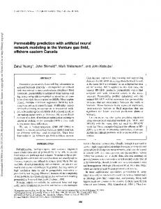
Given the numerous parameters of the conventional models and the complexity of the parameters calibration process, a very effective, efficient method was proposed in this paper based on an artificial neural network, which not only has a higher accuracy, but also eliminates the parameters calibration process. In this section, at first, a definition of this feed-forward neural network method is presented, then the dataset used in this study will be introduced. 3.1 Neural networks algorithm Since 1990s, there has been a gained interest concerning artificial neural networks in variety of disciplines (Dougherty, 1995; Kalogirou, 2000; Kalyoncuoglu and Tigdemir, 2004; Karlaftis and Vlahogianni, 2011). Typically, two merits contribute to the popularity of neural networks. One virtue is that neural networks are capable to handle noisy data and estimate any degree of complexity in non-linear systems (Kalogirou, 2000). The other virtue is that, they do not require any simplifying hypothesis or prior knowledge of problem solving, in comparison with statistical models (Kalyoncuoglu and Tigdemir, 2004; Karlaftis and Vlahogianni, 2011). In terms of the topic discussed in this study, driver–vehicle reaction delay and car following are two complicated concepts. Although there are some findings in previous studies, it is not clear what factors impact the reaction delay and car-following behavior, as well as what their underlying relationships are. Therefore, by virtue of the above mentioned features, we believe that neural networks are more flexible than statistical approaches. In fact, validation results in Section 4 also confirm our judgment. A neural network is a massively parallel distributed processor that has a natural propensity for storing experiential knowledge and making it available for use (Haykin 1999). It stimulates the human brain in two respects: the knowledge is acquired by the network through a learning process, and inter-neuron connection strengths, known as synaptic weights, are used to store the knowledge. A schematic diagram of a typical multilayer neural network is displayed in Figure.1.
This contribution has been peer-reviewed. doi:10.5194/isprsarchives-XL-1-W5-577-2015
578
The International Archives of the Photogrammetry, Remote Sensing and Spatial Information Sciences, Volume XL-1/W5, 2015 International Conference on Sensors & Models in Remote Sensing & Photogrammetry, 23–25 Nov 2015, Kish Island, Iran
should last for at least 30 seconds (Kim et al., 2003; Kim and Taehyung, 2005). After the preliminary study of the noise in the acceleration data taken from the dataset (Punzo et al., 2011) it was found that the use of the moving average method reduced this noise as much as possible. Sixty percent of the data was entered into the designed neural network as training data, 20 percent as testing data, and 20 percent as evaluation data. 3.3 Experimental result
Figure 1.The schematic diagram of a two-layer neural network In this study the network is composed of inputs and two layers. The last layer of a neural network is also called the output layer. The input vector consists of R elements q1, q2… qR. Each input element qi is multiplied by a weight wj, i 1 to form wj, i 1, one of the terms that is sent to the adder. The other input, the constant 1, is multiplied by a bias bj1 and then passed to the adder. The adder output is: R
n j w j , i qi b j , 1
1
1
(7)
i 1
Often recourse to as the net input, goes into the transfer function f 1, which produces the neuron output aj1 in the layer one. The bias bj1 has the effect of increasing or decreasing the net input of the transfer function, depending on whether it is positive or negative, respectively. L1 shows the number of neurons adopted in layer one. If we relate the artificial neural network to a biological neuron, the strength of a synapse is shown by the weights and bias wj, i 1, bj1. A cell body is represented by the adder and transfer function, and the neuron output aj1 represents the signal on an axon. In the same way, handling the outputs of layer one as the inputs of layer two, the signals from layer one are passed through second layer. The transfer function in layer two f 2 can be totally vary from that in
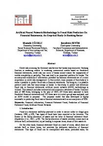
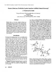
In this paper, in order to determine a trajectory model for vehicle movements, a multilayer neural network approximator was used with 10 neurons in one hidden layer, one neuron in output layer, and Levenberg-Marquardt (Vogl et al., 1988) backpropagation training algorithm. The hyperbolic tangent sigmoid function (Vogl et al., 1988) and purelin function (Vogl et al., 1988) were employed as the transfer functions of the neurons of hidden layer and the output layer, respectively. One of the important aspects in identifying driver behavior is reaction time. This parameter shows the period between the time the driver recognizes a stimulus and the time a suitable response is shown to that stimulus. One of the very popular models that are used for calculating reaction time is the Ozaki model that calculates this parameter separately for the two states of acceleration and deceleration (Ozaki, 1993). In this research, the inputs for determining the trajectory model are the distance between the two cars being followed at any instant, the speed of the leading car, and the difference between the speeds of the two cars. In addition, the reaction time of the driver was calculated using the Ozaki model and was considered as the new input. As will later be shown, the effects of this parameter are very important in modeling trajectories of car movements using the proposed artificial neural network approximator. Figure.2 and Figure.3 demonstrate the fitting curve between the real data and prediction of the proposed model by neglecting the reaction time and by considering it, respectively.
the first layer. The outputs of second layer ak2 k [1, 2,..., L2 ] , are also the outputs of the discussed neural network. L2 shows the number of neurons used in layer two. The neuron network is written in the following matrix form: a f ( w q b ), a f ( w a b ), 1
1
1
1
2
2
2 1
2
(8)
where w1, w2 are the weight matrixes and q, b1, b2, a1, a2 denote the input, bias and output vectors in layers one and two. 3.2 Dataset The actual data on car following from the NGSIM project was used to determine the performance of the proposed model. This dataset was used for the purpose of expanding behavioral algorithm in micro simulation. One part of this dataset is related to the Emeryville Highway and includes routes of about 1500 cars including about 1.5 million information records for the first 15 minutes between 5:00 p.m. and 5:15 p.m. on April 13, 2005. Every record contains 18 information fields taken by the sensors embedded for this purpose at 0.1-second intervals, and the most important fields include accurate spatial position, speed, acceleration, and distance to the car in front. From among all the data, a suitable sample was considered that included three important conditions: both cars should be of the same type, none of them should change lanes during car following, and no other car should come between them. Finally, the car following
Figure 2. Artificial Neural Network prediction without considering the reaction time
This contribution has been peer-reviewed. doi:10.5194/isprsarchives-XL-1-W5-577-2015
579
The International Archives of the Photogrammetry, Remote Sensing and Spatial Information Sciences, Volume XL-1/W5, 2015 International Conference on Sensors & Models in Remote Sensing & Photogrammetry, 23–25 Nov 2015, Kish Island, Iran
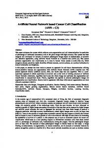
Figure 3. Artificial Neural Network prediction by considering the instantaneous reaction Time Figure.4 demonstrates histogram error of training, testing, and validation data. The proposed ANN model was stopped after 23 epoch. Figure.5 shows the epoch gained the best accuracy. The reason of training stopping was based on achieving the best accuracy goal. Furthermore, if there is not any better accuracy after 310 epochs, training process of the proposed ANN will be finished.
Figure 6. Difference between the real data and two conventional model (Helly and Gipps) 4. VALIDATION OF METHODOLOGY Three measures were employed to validate the proposed methodology. The first measure is the mean square error, Eq. (9). The second measure is the Index of agreement, Eq. (10). Moreover, micro simulation validation was carried out as the last measure. 4.1 Statistical validation To demonstrate the accuracy of the proposed model, the following criteria were used: The Mean Square Error (MSE) method was used to determine the accuracy of the model. The following Equation shows the calculations of the measure of accuracy: i 1 y (ti y (ti ') n
MSE
2
(9)
,
n
Figure 4. Error Histogram for the ANN outputs (Lane 1)
Index of agreement, i.e., d, indicates the extent that the predicted values are error-free. The closer the value of this parameter becomes to 1, the better our model of prediction will be. The following Equation shows this index formula (Papanastasiou et al., 2007):
d 1
' 2 n i 1( yi yi ) ' 2 n i 1( yi y yi y )
(10)
where y ti ' is the value predicted by the model, y ti is the real value or the test data value and y is the mean values of real data. The following table summarizes the statistical results of the model for various states.
Figure 5. The best validation performance (Lane 1) The outputs of the conventional models were then compared to the outputs of the proposed method in Figure.6.
Mean Square Error(MSE) Lane 1 Lane 2 Lane 3 ANN without Reaction 0.347 0.223 0.150 Time ANN with Reaction Time 1.0E-08 7.0E-08 1.0E-08 Helly 2.242 0.988 1.500 Gipps 0.423 0.581 0.295 Table 1. The mean squared error (MSE) between the real data and the output of models with reaction time and without it
This contribution has been peer-reviewed. doi:10.5194/isprsarchives-XL-1-W5-577-2015
580
The International Archives of the Photogrammetry, Remote Sensing and Spatial Information Sciences, Volume XL-1/W5, 2015 International Conference on Sensors & Models in Remote Sensing & Photogrammetry, 23–25 Nov 2015, Kish Island, Iran
Index of Agreement Lane1
Lane 2
Lane 3
0.55%
0.89%
0.85%
0.99%
0.99%
0.99%
Helly
0.17%
0.41%
0.37%
Gipps
0.38%
0.34%
0.34%
ANN without Reaction Time ANN with Reaction Time
Simulation was performed with 0.1-second steps and it was found that the proposed model has a good validity according to the proximity to the real situation of car-following in its simulation. Figure .18 depicts simulation results in three lane.
Table 2. Statistical summary for each observed and simulated vehicle (d is index of agreement) Based on the above table and by considering the instantaneous reaction, the proposed model yields the best statistical parameters for all lines of the route. This model can be used for the car guidance systems in the non-collision state. 4.2 Microscopic validation In this section, we show the validity of the proposed model using the micro-simulation technique. After determining the model accuracy using the error test with the least squares error method and the use of index of agreement parameter as the determinant of prediction accuracy in the previous section, we firstly considered Highway Emeryville and three lines, where data was collected. The following figure shows the study area for simulation:
Figure 8. Simulation prototype 5. CONCLUSION Car-following models are among the most important topics in the field of traffic simulation at the micro level. All famous models that are used today include a set of parameters that require careful calibration, and any changes, even trivial, will severely affect the output. To solve this problem, this paper uses an artificial neural network to propose a car-following model. The model predicts the desired output, i.e. acceleration changes, by allocating four parameters, including the speed of the front car, the relative distance to the front car, the relative speed between the front car, and the follower car with different reaction times. To demonstrate the validity of this model, two methods were used: theory of errors and micro simulation. In the theory of errors, the output data of the models were compared with reality and it was found that the proposed model has a good accuracy in the car-following modeling, considering the instantaneous reaction time as an input parameter. In the simulation, it was shown that the results from the moving vehicles in the actual route follow the actual conditions of the car-following flow, based on the understanding of the follower car's driver about the performance of the front car, including the car speed and distance with it in every 0.1 seconds. This model can also be used in driver support tools, maintaining the safe distance, guiding unmanned vehicles and other applications of intelligent transportation systems. REFERENCES Brackstone, M. and M. McDonald. 1999. "Car-following: a historical review." Transportation Research Part F: Traffic Psychology and Behaviour 2(4): 181-196.
Figure 7. Study area During the simulation, two cars were assumed for each line: one as the front car and the other as the follower car. The front car started moving with the speed available at the collected data and the follower car instantaneously calculated acceleration based on the proposed model by understanding the speed of the front car, their distance, and relative speed. Based on this acceleration, displacement was calculated for the next moment.
Chakroborty, P. and S. Kikuchi., 1999. "Evaluation of the General Motors based car-following models and a proposed fuzzy inference model." Transportation Research Part C: Emerging Technologies 7(4): 209-235. Cho, H.-J, and Y.-T. Wu., 2008. "Microscopic analysis of desired-speed car-following stability." Applied Mathematics and Computation 196(2): 638-645.
This contribution has been peer-reviewed. doi:10.5194/isprsarchives-XL-1-W5-577-2015
581
The International Archives of the Photogrammetry, Remote Sensing and Spatial Information Sciences, Volume XL-1/W5, 2015 International Conference on Sensors & Models in Remote Sensing & Photogrammetry, 23–25 Nov 2015, Kish Island, Iran
Dougherty, M., 1995. "A review of neural networks applied to transport." Transportation Research Part C: Emerging Technologies 3(4): 247-260.
Panwai, S. and H. Dia., 2007. "Neural agent car-following models." Intelligent Transportation Systems, IEEE Transactions on 8(1): 60-70.
Gazis, D. C., R. Herman and R. B. Potts., 1959. "Car-following theory of steady-state traffic flow." Operations research 7(4): 499-505.
Papanastasiou, D., D. Melas and I. Kioutsioukis., 2007. "Development and assessment of neural network and multiple regression models in order to predict PM10 levels in a mediumsized Mediterranean city." Water, air, and soil pollution 182(14): 325-334.
Gipps, P. G., 1981. "A behavioural car-following model for computer simulation." Transportation Research Part B: Methodological 15(2): 105-111. Helly, W., 1961. Simulation of bottlenecks in single-lane traffic flow. Herman, R., E. W. Montroll, R. B. Potts and R. W. Rothery., 1959. "Traffic dynamics: analysis of stability in car following." Operations research 7(1): 86-106. Herman, R. and R. B. Potts., 1900. "Single lane traffic theory and experiment." Herman, R. and R. Rothery., 1967. PROPAGATION OF DISTURBANCES IN VEHICULAR PLATOONS. IN VEHICULAR TRAFFIC SCIENCE. Proceedings of the Third International Symposium on the Theory of Traffic Flow. Herman, R. and R. W. Rothery., 1965. Car following and steady-state flow. Proceedings of the 2nd International Symposium on the Theory of Traffic Flow. Ed J. Almond, OECD, Paris. Haykin, S., 1999. "Neural Networks–A Comprehensive Foundation." New Jersey: Printice-Hall Inc. Kalogirou, S. A., 2000. "Applications of artificial neuralnetworks for energy systems." Applied Energy 67(1): 17-35. Kalyoncuoglu, S. F. and M. Tigdemir., 2004. "An alternative approach for modelling and simulation of traffic data: artificial neural networks." Simulation Modelling Practice and Theory 12(5): 351-362.
Pipes, L. A., 1953. "An operational analysis of traffic dynamics." Journal of applied physics 24(3): 274-281. Punzo, V., M. T. Borzacchiello and B. Ciuffo., 2011. "On the assessment of vehicle trajectory data accuracy and application to the Next Generation SIMulation (NGSIM) program data." Transportation Research Part C: Emerging Technologies 19(6): 1243-1262. Rahman, M. 2013. "Application of parameter estimation and calibration method for car-following models". Master of Science Thesis, Clemson University. Reuschel, A., 1950. "Vehicle movements in a platoon." Oesterreichisches Ingenieur-Archir 4: 193-215. Saifuzzaman, M. and Z. Zheng., 2014. "Incorporating humanfactors in car-following models: a review of recent developments and research needs." Transportation research part C: emerging technologies 48: 379-403. Vogl, T. P., J. Mangis, A. Rigler, W. Zink and D. Alkon., 1988. "Accelerating the convergence of the back-propagation method." Biological cybernetics 59(4-5): 257-263. Wilson, R. E. 2001. "An analysis of Gipps's car‐following model of highway traffic". IMA journal of applied mathematics, 66, 509-537. Wu, J., Y. Sui and T. Wang., 2009. "Intelligent transport systems in China." Proceedings of the ICE-Municipal Engineer 162(1): 25-32.
Karlaftis, M. and E. Vlahogianni., 2011. "Statistical methods versus neural networks in transportation research: Differences, similarities and some insights." Transportation Research Part C: Emerging Technologies 19(3): 387-399. Kim, T., 2005. "Analysis of Variability in Car-Following Behavior over Long-Term Driving Maneuvers." Kim, T., D. J. Lovell and Y. Park., 2003. Limitations of previous models on car-following behavior and research needs. 82nd Annual Meeting of the Transportation Research Board, Washington, DC. Kometani, E. and T. Sasaki., 1959. "A safety index for traffic with linear spacing." Operations Research 7(6): 704-720. Ma, X. and I. Andreasson., 2007. "Behavior measurement, analysis, and regime classification in car following." Intelligent Transportation Systems, IEEE Transactions on 8(1): 144-156. Ozaki, H., 1993. "REACTION AND ANTICIPATION IN THE CAR-FOLLOWING BEHAVIOR." Transportation and traffic theory.
This contribution has been peer-reviewed. doi:10.5194/isprsarchives-XL-1-W5-577-2015
582