Multi-mode bosonic Gaussian channels

Multi-mode bosonic Gaussian channels arXiv:0804.0511v3 [quant-ph] 6 Aug 2008

F. Caruso1, J. Eisert2 , V. Giovannetti1 , and A.S. Holevo3 1

NEST CNR-INFM & Scuola Normale Superiore, Piazza dei Cavalieri 7, I-56126 Pisa, Italy 2

Institute for Mathematical Sciences, Imperial College London, London SW7 2PE, UK 3 Steklov

Mathematical Institute, Gubkina 8, 119991 Moscow, Russia

August 6, 2008 Abstract A complete analysis of multi-mode bosonic Gaussian channels is proposed. We clarify the structure of unitary dilations of general Gaussian channels involving any number of bosonic modes and present a normal form. The maximum number of auxiliary modes that is needed is identified, including all rank deficient cases, and the specific role of additive classical noise is highlighted. By using this analysis, we derive a canonical matrix form of the noisy evolution of n-mode bosonic Gaussian channels and of their weak complementary counterparts, based on a recent generalization of the normal mode decomposition for non-symmetric or locality constrained situations. It allows us to simplify the weak-degradability classification. Moreover, we investigate the structure of some singular multi-mode channels, like the additive classical noise channel that can be used to decompose a noisy channel in terms of a less noisy one in order to find new sets of maps with zero quantum capacity. Finally, the two-mode case is analyzed in detail. By exploiting the composition rules of two-mode maps and the fact that anti-degradable channels cannot be used to transfer quantum information, we identify sets of two-mode bosonic channels with zero capacity.

Contents 1 Multi-mode bosonic Gaussian channels 1.1 Notation and preliminaries . . . . . . . . . . . . . . . . . . . . . . 1.2 Bosonic Gaussian channels . . . . . . . . . . . . . . . . . . . . . . 2 Unitary dilation theorem 2.1 General dilations . . . . . . . . . . . . . . . 2.2 Reducing the number of environmental modes 2.3 Minimal noise channels . . . . . . . . . . . . 2.4 Additive classical noise channel . . . . . . . 2.5 Canonical form for generic channels . . . . . 1

. . . . .

. . . . .

. . . . .

. . . . .

. . . . .

. . . . .

. . . . .

. . . . .

. . . . .

. . . . .

. . . . .

. . . . .

3 3 5 7 7 14 16 18 18

3 Weak degradability 3.1 A criterion for weak degradability . . . . . . . . . . . . . . . . . .

20 21

4 Two-mode bosonic Gaussian channels 4.1 Weak-degradability properties . . . . . . . . . . . . . . . . . . . . 4.2 Channels with zero quantum capacity . . . . . . . . . . . . . . . .

23 25 27

5 Conclusions

28

6 Acknowledgements

29

A Proof of Lemma 1

29

B Derivation of Eq. (35)

30

C Properties of the environmental states C.1 Solution for ℓpure = 2n − r ′ /2 environmental modes . . . . . . . . . C.2 Solution for ℓ = 2n − r/2 not necessarily pure environmental modes

31 31 33

D Equivalent unitary dilations

33

E The ideal-like quantum channel

35

Bosonic Gaussian channels are ubiquitous in physics. They arise whenever a harmonic system interacts linearly with a number of bosonic modes which are inaccessible in principle or in practice [1, 2, 3, 4, 5, 6, 7]. They provide realistic noise models for a variety of quantum optical and solid state systems when treated as open quantum systems, including models for wave guides and quantum condensates. They play a fundamental role in characterizing the efficiency of a variety of tasks in continuousvariables quantum information processing [8], including quantum communication [9] and cryptography [10]. Most importantly, communication channels such as optical fibers can to a good approximation be described by Gaussian quantum channels. Not very surprisingly in the light of the central status of such quantum channels, a lot of effort has been recently devoted to studying their properties (see Ref. [4] for a review), based on a long tradition of work on Gaussian channels [6, 2, 3]. Specifically, from a quantum information perspective, a key question is whether or not a channels allows for the reliable transmission of classical or quantum information [3, 4, 11, 12, 13, 14, 15, 16, 17, 18]. Significant progress has been made in this respect in recent years, although for some important cases, like the thermal noise channel modelling a realistic fiber with offset noise, the quantum capacity is still not yet known. In this context, the degradability properties represent a powerful tool to simplify the quantum capacity issue of such Gaussian channels. Indeed, in Refs. [16, 17] it has been shown that with some (important) exceptions, Gaussian channels which operate on a single bosonic mode (i.e., one-mode Gaussian channels) can be classified as weakly degradable or anti-degradable. This paved the way for the solution of 2

the quantum capacity [19] for a large class of these maps [15]. Here, first we propose a general construction of unitary dilations of multi-mode quantum channels, including all rank-deficient cases. We characterize the minimal noise maps involving only true quantum noise. Then, by using a generalized normal mode decomposition recently introduced in Ref. [20], we generalize the results of Refs. [16, 17] concerning Gaussian weak complementary channels to the multimode case giving a simple weak-degradability/anti-degradability condition for such channels. The paper ends with a detailed analysis of the two-mode case. This is important since any n-mode channel can always be reduced to single-mode and twomode components [20]. We detalize the degradability analysis and investigate a useful decomposition of a channel with the additive classical noise map that allows us to find new sets of channels with zero quantum capacity.

1 Multi-mode bosonic Gaussian channels Gaussian channels arise from linear dynamics of open bosonic system interacting with a Gaussian environment via quadratic Hamiltonians. Loosely speaking, they can be characterized as CPT maps that transform Gaussian states into Gaussian states [21, 22].

1.1 Notation and preliminaries Consider a system composed by n bosonic modes having canonical coordinates ˆ 1 , Pˆ1 , · · · , Q ˆ n , Pˆn . The canonical commutation relations of the canonical coordiQ ˆ := (Q ˆ1, · · · , Q ˆ n ; Pˆ1 , · · · , Pˆn ), are grasped by ˆj , R ˆ j ′ ] = i(σ2n )j,j ′ , where R nates, [R the 2n × 2n commutation matrix   0 11n , (1) σ2n = −11n 0 when this order of canonical coordinates is chosen, (here 11n is the n × n identity ˆ will not matrix) [3, 4, 21]. Even though different reordering of the elements of R affect the definitions that follow, we find it useful to assume a specific form for σ2n . One defines the group of real symplectic matrices Sp(2n, ) as the set of 2n × 2n real matrices S which satisfy the condition

R

Sσ2n S T = σ2n .

(2)

−1 Since Det[σ2n ] = 1, and σ2n = −σ2n , any symplectic matrix S has Det[S] = 1 −1 and it is invertible with S ∈ Sp(2n, ). Similarly, one has S T ∈ Sp(2n, ). Symplectic matrices play a key role in the characterization of bosonic systems. Inˆ deed, define the Weyl (displacement) operators as Vˆ (z) = Vˆ † (−z) := exp[iRz] with z := (x1 , x2 , · · · , xn , y1 , y2 , · · · , yn )T being a column vector of 2n . Then it is possible to show [1] that for any S ∈ Sp(2n, ) there exists a canonical unitary transformation Uˆ which maps the canonical observables of the system into a linear ˆ j , satisfying the condition combination of the operators R

R

R

R

Uˆ † Vˆ (z) Uˆ = Vˆ (Sz) , 3

R

(3)

for all z. This is often referred to as metaplectic representation. Conversely, one can ˆ which transforms Vˆ (z) as in Eq. (3) must correspond to an show that any unitary U S ∈ Sp(2n, ). Weyl operators allow one to rewrite the canonical commutation relations as

R

Vˆ (z)Vˆ (z ′ ) = exp[− 2i z T σ2n z ′ ]Vˆ (z + z ′ ) ,

(4)

and permit a complete descriptions of the system in terms of (characteristic) comˆ (in particular, any density plex functions. Specifically, any trace-class operator Θ operator) can be expressed as Z 2n d z ˆ ˆ z) Vˆ (−z) , Θ= φ(Θ; (5) (2π)n ˆ z) is the characteristic function assowhere d2n z := dx1 · · · dxn dy1 · · · dyn and φ(Θ; ˆ defined by ciated with the operator Θ ˆ z) := Tr[ Θ ˆ Vˆ (z) ] . φ(Θ;

(6)

Within this framework a density operator ρˆ of the n modes is said to represent a Gaussian state if its characteristic function φ(ˆ ρ; z) has a Gaussian form, i.e., φ(ˆ ρ; z) = exp[− 41 z T γz + imT z] ,

(7)

ˆ j ], and the 2n × 2n real with m being a real vector of mean values mj := Tr[ ρˆ R symmetric matrix γ being the covariance matrix [1, 4, 7] of ρˆ. For generic density operators ρˆ (not only the Gaussian ones) the latter is defined as the variance of the ˆ i.e., canonical coordinates R, h  i (8) γj,j ′ := Tr ρ (Rj − mj ), (Rj ′ − mj ′ ) , with {·, ·} being the anti-commutator, and it is bound to satisfy the uncertainty relations γ > iσ2n ,

(9)

with σ2n being the commutation matrix (1). Up to an arbitrary vector m, the uncertainty inequality presented above uniquely characterizes the set of Gaussian states, i.e. any γ satisfying (9) defines a Gaussian state. Let us first notice that if γ satisfies (9) then it must be (strictly) positive definite γ > 0, and have Det[γ] > 1. From Williamson theorem [23] it follows that there exists a symplectic S ∈ Sp(2n, ) such that   D 0 ST , (10) γ=S 0 D

R

where D := diag(d1 , · · · , dn ) is a diagonal matrix formed by the symplectic eigenvalues dj > 1 of γ. For S = 112n Eq. (10) gives the covariance matrix associated with 4

thermal bosonic states. This also shows that any covariance matrix γ satisfying (9) can be written as γ = SS T + ∆ ,

(11)

with ∆ > 01 . The extremal solutions of Eq. (11), i.e., γ = SS T , are minimal uncertainty solutions and correspond to the pure Gaussian states of n modes (e.g., multi-mode squeezed vacuum states). They are uniquely determined by the condition Det[γ] = 1 and satisfy the condition [18] γ = −σ2n (γ −1 )σ2n .

(13)

1.2 Bosonic Gaussian channels In the Schr¨odinger picture evolution is described by applying the transformation to the states (i.e., the density operators), ρˆ 7→ Φ(ˆ ρ). In the Heisenberg picture the transformation is applied to the observables of the system, while leaving the ˆ 7→ ΦH (Θ). ˆ The two pictures are related through the identity states unchanged, Θ ˆ = Tr[ˆ ˆ which holds for all ρˆ and Θ. ˆ The map ΦH is called the Tr[Φ(ˆ ρ)Θ] ρΦH (Θ)], dual of Φ. Due to the representation (5) and (6) any completely positive, trace preserving (CPT) transformation on the n-modes can be characterized by its action on the Weyl operators of the system in the Heisenberg picture (e.g., see Ref. [17]). In particular, a bosonic Gaussian channel (BGC) is defined as a map which, for all z, operates on V (z) according to [3] Vˆ (z) 7−→ ΦH (Vˆ (z)) := Vˆ (Xz) exp[− 14 z T Y z + iv T z] ,

R

(14)

R

with v being some fixed real vector of 2n , and with Y, X ∈ 2n×2n being some fixed real 2n × 2n matrices satisfying the complete positivity condition Y > iΣ

with Σ := σ2n − X T σ2n X .

(15)

In the context of BGCs the above inequality is the quantum channel counterpart of the uncertainty relation (9). Indeed up to a vector v, Eq. (15) uniquely determines the set of BGCs and bounds Y to be positive-semidefinite, Y > 0. However, differently from (9) in this case strict positivity is not a necessary prerequisite for Y . A completely positive map defined by Eqs. (14) and (15) will be referred to as bosonic Gaussian channel (BGC). As mentioned before, such a map is a model for a wide class of physical situations, ranging from communication channels such as optical fibers, to open quantum systems, and to dynamics in harmonic lattice systems. Whenever one has only partial access to the dynamics of a system that can be well-described 1

This is indeed the matrix ∆ := S



D − 11n 0

0 D − 11n

with D as in Eq. (10) which is positive since D > 11n .

5



ST

(12)

by a time evolution governed by a Hamiltonian that is a quadratic polynomial in the canonical coordinates, one will arrive at a model described by Eqs. (14) and (15)2 . An important subset of the BGCs is given by set of Gaussian unitary transformations which have Y = 0, X ∈ Sp(2n, ), and v arbitrary. They include the canonical transformations of Eq. (3) (characterized by v = 0), and the displacement transformations (characterized by having X = 112n and v arbitrary). The latter simply adds a phase to the Weyl operators and correspond to unitary transformations of the form ΦH (Vˆ (z)) := Vˆ (−v)Vˆ (z)Vˆ (v) = Vˆ (z) exp[iv T z]. In the Schr¨odinger picture the BGC transformation (14) induces a mapping of the characteristic functions of the form

R

φ(ˆ ρ; z) 7−→ φ(Φ(ˆ ρ); z) := φ(ˆ ρ; Xz) exp[− 41 z T Y z + iv T z] ,

(16)

which in turn yields the following transformation of the mean and the covariance matrix m − 7 → XT m + v , γ − 7 → X T γX + Y .

(17)

Clearly, BGCs always map Gaussian input states into Gaussian output states. For purposes of assessing quantum or classical information capacities, output entropies, or studying degradability or anti-degradability of a channel [16, 17, 14, 15], the full knowledge of the channel is not required: Transforming the input or the output with any unitary operation (say, Gaussian unitaries) will not alter any of these quantities. It is then convenient to take advantage of this freedom to simplify the description of the BGCs. To do so we first notice that the set of Gaussian maps is closed under composition. Consider then Φ′ and Φ′′ two BGCs described respectively by the elements X ′ , Y ′ , v ′ and X ′′ , Y ′′ , v ′′ . The composition Φ′′ ◦ Φ′ where, in Schr¨odinger representation, we first operate with Φ′ and then with Φ′′ , is still a BGC and it is characterized by the parameters v = (X ′′ )T v ′ + v ′′ , X = X ′ X ′′ , Y = (X ′′ )T Y ′ X ′′ + Y ′′ .

(18)

Exploiting these composition rules it is then easy to verify that the vector v can always be compensated by properly displacing either the input state or the output state (or both) of the channel. For instance by taking X ′′ = 112n , Y ′′ = 0 and v ′′ = −v ′ , Eq. (18) shows that Φ′ is unitarily equivalent to the Gaussian channel Φ which has v = 0 and X = X ′ , Y = Y ′ . Therefore, without loss of generality, in the following we will focus on BGCs having v = 0. More generally consider the case where we cascade a generic BGC Φ′ described by matrices X ′ , Y ′ as in Eq. (15) with a couple of canonical unitary transformation Uˆ1 and Uˆ2 described by the symplectic matrices S1 and S2 respectively. The resulting 2

This set does not contain ideal Gaussian measurements, like optical homodyning [31].

6

BGC Φ is then described by the matrices X = S1 (X ′ )S2 , Y = S2T (Y ′ )S2 .

(19)

For single mode (n = 1) this procedure induces a simplified canonical form [13, 17, 14] which, up to a Gaussian unitarily equivalence, allows one to focus only on transformations characterized by X and Y which, apart from some special cases, are proportional to the identity. In this paper we will generalize some of these results to an arbitrary number of modes n. To achieve this goal, in the following section we first present an explicit dilation representation in which the mapping (14) is described as a (canonical) unitary coupling between the n modes of the system and some extra environmental modes which are initially prepared into a Gaussian state. Then we will introduce the notion of minimal noise channel, showing a useful decomposition rule.

2 Unitary dilation theorem In this section we introduce a general construction of unitary dilations of multi-mode quantum channels. Specifically we show that a CPT channel acting on n modes is a BGC if and only if it can be realized by invoking ℓ 6 2n additional (environmental) modes E through the expression ˆ ρ ⊗ ρˆE )Uˆ † ] , Φ(ˆ ρ) = TrE [U(ˆ

(20)

where ρˆ is the input n-mode state of the system, ρˆE is a Gaussian state of an environment, Uˆ is a canonical unitary transformation which couples the system with the environment, and TrE denotes the partial trace over E. In case in which ρˆE is pure, Eq. (20) corresponds to a Stinespring dilation [24] of the channel Φ, otherwise it is a physical representation analogous to those employed in Refs. [16, 17] for the single mode case.

2.1 General dilations In this subsection, we will construct Gaussian dilations, including a discussion of all rank-deficient cases, and will later focus on dilations involving the minimal number of modes. To proceed, we will first establish some conventions and notation. To start with, we write the commutation matrix of our n + ℓ modes in the block structure   σ2n 0 } 2n E (21) σ := σ2n ⊕ σ2ℓ = E 0 σ2ℓ } 2ℓ , E where σ2n and σ2ℓ are 2n × 2n and 2ℓ × 2ℓ commutation matrices associated with the system and environmental modes, respectively. For σ2n we assume the structure E as defined in Eq. (1). For σ2ℓ , in contrast, we do not make any assumption at this

7

point, leaving open the possibility of defining it later on3 . Accordingly, the canonical unitary transformation Uˆ of Eq. (20) will be uniquely determined by a 2(n + ℓ) × 2(n + ℓ) real matrix S ∈ Sp(2(n + ℓ), ) of block form   s1 s2 , (22) S := s3 s4

R

which satisfies the condition

SσS T = σ ,

⇐⇒

 E T s1 σ2n sT1 + s2 σ2ℓ s2 = σ2n ,      E T s4 = 0 , s1 σ2n sT3 + s2 σ2ℓ      E T E s3 σ2n sT3 + s4 σ2ℓ s4 = σ2ℓ .

(23)

In the above expressions, s1 and s4 are 2n × 2n and 2ℓ × 2ℓ real square matrices, while s2 and sT3 are 2n×2ℓ real rectangular matrices. Introducing then the covariance E matrices γ > iσ2n and γE > iσ2ℓ of the states ρˆ and ρˆE , the identity (20) can be written as   γ 0 (24) S S T = s1 γ sT1 + s2 γE sT2 = X T γX + Y, 0 γE 2n where |2n denotes the upper principle submatrix of degree 2n, and where X, Y ∈

R2n×2n satisfying the condition (15) are the matrices associated with the channel Φ.

In writing Eq. (24) we use the fact that due to the definition (21) the covariance matrix of the composite state ρˆ ⊗ ρˆE can be expressed as γ ⊕ γE . With these definitions, the first part of the unitary dilation property (20) can be written as follows:

Proposition 1 (Unitary dilations of Gaussian channels) Let γE be the covariance matrix of a Gaussian state of ℓ modes and let S ∈ Sp(2(n + ℓ), ) be a symplectic transformation. Then there exists a symmetric 2n × 2n-matrix Y > 0 and a 2n × 2nmatrix X satisfying the condition (15), such that Eq. (24) holds for all γ.

R

Proof: The proof is straightforward: We write S in the block form (22) and take X = sT1 and Y = s2 γE sT2 . Since γE is a covariance matrix of ℓ modes, γE − iσ2ℓ > 0 and therefore s2 (γE − iσℓ )sT2 > 0. This leads to Eq. (15) through the identity the symplectic condition s1 σ2n sT1 + s2 σ2ℓ sT2 = σ2n which follows by comparing the upper principle submatrices of degree n of both terms of Eq. (23).  This proves that any CPT map obtained by coupling the n modes with a Gaussian state of ℓ environmental bosonic modes through a Gaussian unitary Uˆ is a BGC. The converse property is more demanding. In order to present it we find it useful to state first the following ˆj , R ˆ j ′ ] = iσj,j ′ With this choice the canonical commutation relations of the n + ℓ mode read as [R ˆ ˆ ˆ ˆ ˆ ˆ ˆ where R := (Q1 , · · · , Qn ; P1 , · · · , Pn ; rˆ1 , · · · , rˆ2ℓ ) with Qj , Pj being the canonical coordinates of the j-th system mode and with and rˆ1 , · · · , rˆ2ℓ being some ordering of the canonical coordinates E ˆE ˆE ˆE ˆE Q 1 , P1 ; · · · ; Qℓ , Pℓ of the environmental modes. For instance, taking σ2ℓ = σ2ℓ corresponds to E E E E ˆ := (Q ˆ 1, · · · , Q ˆ n ; Pˆ1 , · · · , Pˆn ; Q ˆ ,··· ,Q ˆ ; Pˆ , · · · , Pˆ ). have R 1 1 ℓ ℓ 3

8

E Lemma 1 (Extensions of symplectic forms) Let, for some skew symmetric σ2ℓ , s1 and s2 be 2n × 2n and 2n × 2ℓ real matrices forming a symplectic system, i.e., E T s1 σ2n sT1 + s2 σ2ℓ s2 = σ2n . Then we can always find real matrices s3 and s4 such that S of Eq. (22) is symplectic with respect to the commutation matrix (21).

Proof: Since the rows of S form a symplectic basis, given s1 and s2 (an incomplete symplectic basis), it is always possible to find s3 and s4 as above. The proof easily follows from a skew-symmetric version of the Gram-Schmidt process to construct a symplectic basis [25]. For a special subset of BGCs, in Sec. 2.5 we will present an explicit expression for S based on a simplified (canonical) representation of the X matrix that defines Φ. See also Appendix A.  Due to the above result, the possibility of realizing unitary dilation Eq. (20) for a generic BGC described by the matrices X and Y > iΣ = i(σ2n − X T σ2n X), can be proven by simply taking s1 = X T and finding some 2n × 2ℓ real matrix s2 and an E ℓ-mode covariance matrix γE > iσ2ℓ that solve the equations E T s2 σ2ℓ s2 = σ2n − s1 σ2n sT1 = Σ , s2 γE sT2 = Y .

(25) (26)

With this choice in fact Eq. (24) is trivially satisfied for all γ, while s1 and s2 can be completed to a symplectic matrix S ∈ Sp(2(n + ℓ), ). The unitary dilation property (20) can hence be restated as follows:

R

Theorem 1 (Unitary dilations of Gaussian channels: Converse implication) For any real 2n×2n-matrices X and Y satisfying the condition (15), there exist ℓ smaller than or equal to 2n, S ∈ Sp(2(n + ℓ), ), and a covariance matrix γE of ℓ modes, such that Eq. (24) is satisfied.

R

Proof: As already noticed the whole problem can be solved by assuming s1 = X T and finding s2 and γE that satisfy Eqs. (25) and (26). We start by observing that the 2n × 2n matrix Σ defined in Eq. (15) is skew-symmetric, i.e., Σ = −ΣT . Moreover according to Eq. (15) its support must be contained in the support of Y , i.e., Supp[Σ] ⊆ Supp[Y ]. Consequently given k := rank[Y ] and r := rank[Σ] as the ranks of Y and Σ, respectively, one has that k > r. We can hence identify three different regimes: (i) k = 2n, r = 2n, i.e., both Y and Σ are full rank and hence invertible. Loosely speaking, this means that all the noise components in the channel are basically quantum (although may involve classical noise as well). (ii) k = 2n and r < 2n, i.e., Y is full rank and hence invertible, while Σ is singular. This means that the some of the noise components can be purely classical, but still nondegenerate. (iii) 2n > k > r, i.e., both Y and Σ are singular. There are noise components with zero variance. 9

Even though (i) and (ii) admit similar solutions, it is instructive to analyze them separately. In the former case in fact there is a simple direct way of constructing a physical dilation of the channel with ℓ = n environmental modes. (i) Since Σ is skew-symmetric and invertible there exists an O ∈ O(2n, ) orthogonal such that   0 µ T OΣO = , (27) −µ 0

R

where µ = diag(µ1 , · · · , µn ) and µi > 0 for all i = 1, · · · , n (see page 107 in Ref. [26]). Hence K := M −1/2 O with M := µ ⊕ µ satisfies KΣK T = σ2n .

(28)

s2 σ2n sT2 = K −1 σ2n K −T = Σ ,

(29)

Taking then s2 := K −1 we get4

which corresponds to Eq. (25) for ℓ = n. Since s1 = X T , Lemma 1 guarantees that this is sufficient to prove the existence of S. The condition (24) finally follows by taking γE = KY K T which is strictly positive (indeed K is invertible and Y > 0 because it has full rank) and which satisfies the uncertainty relation (9), i.e., Y > iΣ

=⇒

γE = KY K T > iKΣK T = iσ2n .

(30)

This shows that the channel admits a unitary dilation of the form as specified in E Eq. (20) with ℓ = n environmental modes with commutation matrix, σ2n = σ2n – see discussion after Eq. (21). Such a solution, however, will involve a pure state ρˆE only if Det[γE ] = 1, i.e., Det[Y ]Det[K]2 = 1

⇐⇒

Det[Y ] = Det[Σ] .

(31)

When Det[γE ] > 1, i.e., Det[Y ] > Det[Σ], we can still construct a pure dilation by simply adding further n modes which purify the state associated with the covariance ˆ associated with S as the identity matrix γE and by extending the unitary operator U operator on them. For details see the discussion of case (ii) given below. This corresponds to constructing a unitary dilation (20) with the pure state ρˆE being defined on ℓ = 2n modes. (ii) In this case Y is still invertible, while Σ is not. Differently from the approach we adopted in solving case (i), we here derive directly a Stinespring unitary dilation, i.e., we construct a solution with a pure γE that involves ℓ = 2n environmental modes. In the next section, however, we will show that, dropping the purity requirement, one can construct unitary dilation that involves ρˆE with only ℓ = 2n − r/2 modes. 4

From now on, the symbol A−T will be used to indicate the transpose of the inverse of the matrix A, i.e., A−T := (A−1 )T = (AT )−1 .

10

To find s2 and γE which solve Eqs. (25) and (26), it is useful to first transform Y into a simpler form by a congruent transformation, i.e., CY C T = 112n ,

(32)

R

with C ∈ Gl(2n, ) being not singular, e.g., C := Y −1/2 . From Eq. (15) it then follows that 112n > iΣ′ , (33) with Σ′ := Y −1/2 Σ Y −1/2 being skew-symmetric (i.e., Σ′ = −(Σ′ )T ) and singular with rank[Σ′ ] = rank[Σ] = r [26]. We then observe that introducing s2 = Y 1/2 s′2 ,

(34)

the conditions (25) and (26) can be written as E s′2 σ2ℓ (s′2 )T = Σ′ , s′2 γE (s′2 )T = 112n .

(35) (36)

Finding s′2 and γE which satisfy these expressions will provide us also a solution of Eqs. (25) and (26). As in the case of Eq. (27), there exists an orthogonal matrix O ∈ O(2n, ) which transforms the skew-symmetric matrix Σ′ in a simplified block form. In this case however, since Σ′ is singular, we find [26]   µ 0 } r/2 0   0 0  } n − r/2 OΣ′ O T =  (37)  −µ  } r/2 0 0 } n − r/2, 0 0

R

where now µ = diag(µ1 , · · · , µr/2 ) is the r/2 × r/2 diagonal matrix formed by the strictly positive eigenvalues of |Σ′ | which satisfy the conditions 1 > µj > 0, this being equivalent with 11r/2 > µ, (38) as a consequence of inequality (33). Define then K := M −1/2 O with   0 µ } r/2 0   0 11n−r/2  } n − r/2 M =   } r/2 µ 0 0 } n − r/2. 0 11n−r/2

(39)

It satisfies the identity

KΣ′ K T



0   =  −11r/2 0

0 0

11r/2

0 0 0

0

11



} r/2  } n − r/2   } r/2 } n − r/2.

(40)

E To show that Eqs. (35) and (36) admit a solution we take ℓ = 2n and write σ4n = σ2n ⊕σ2n = σ4n with σ2n as in Eq. (1). With these definitions the 2n×4n rectangular matrix s′2 can be chosen to have the block structure   −1 OT A , K (41) s′2 =

with A being the following 2n × 2n symmetric matrix  0 0 0  0 11n−r/2 A = AT =   0 0 0 0 11n−r/2



} r/2  } n − r/2   } r/2 } n − r/2.

(42)

By direct substitution one can easily verify that Eq. (35) is indeed satisfied, see Appendix B for details. Inserting Eq. (41) into Eq. (36) yields now the following equation α + A δ T + δ AT + A β AT = M −1 ,

(43)

for the 4n × 4n covariance matrix γE =



α δ δT β



,

see Appendix C for details. A solution can be easily derived by taking   µ−1 0 } r/2 0   0 ξ 1 1 n−r/2  } n − r/2 α=β=   } r/2 µ−1 0 0 } n − r/2, 0 ξ 11n−r/2

with ξ = 5/4 and   δ= 

f (µ−1 ) 0

0

f (µ−1 ) 0

0 f (ξ 11n−r/2 )

 0 } r/2  f (ξ 11n−r/2 )  } n − r/2  } r/2 0 } n − r/2,

(44)

(45)

(46)

with f (θ) := −(θ2 − 11)1/2 . For all diagonal matrices µ compatible with the constraint (38) the resulting γE satisfies the uncertainty relation γE > iσ4n . Moreover since it has Det[γE ] = 1, this is also a minimal uncertainty state, i.e., a pure Gaussian state of 2n modes. It is worth stressing that for r = 2n, i.e., when also the rank of Σ is maximum, the above solution provides an alternative derivation of the unitary dilation discussed in the part (i) of the theorem. In this case the covariance matrix γE has block elements     −1 }n 0 f (µ−1) }n µ 0 , (47) , δ= α=β= −1 −1 }n f (µ ) 0 }n 0 µ 12

where µ is now a strictly positive n × n matrix, while Eqs. (34) and (41) yield   1/2 0 0 0 µ }n 1/2 T (48) s2 := Y O 1/2 } n. 0 0 0 µ (iii) Here both Y and Σ are singular. This case is very similar to case (ii). Here, the dilation can be constructed by introducing a strictly positive matrix Y¯ > 0 which satisfies the condition Π Y¯ Π = Y ,

(49)

with Π being the projector onto the support of Y . Such a Y¯ always exists (Y¯ = Y + (11 − Π)). By construction, it satisfies the inequality Y¯ > Y > iΣ. According to Sec. 1.2, Y¯ and X define thus a BGC. Moreover, since Y¯ is strictly positive, it has full rank. Therefore, we can use part (ii) of the proof to find a 2n × 2ℓ matrix s¯2 and γ¯E > iσ2ℓ which satisfy the conditions (25) and (26), i.e. E T s¯2 σ2ℓ s¯2 = Σ , s¯2 γ¯E s¯T2 = Y¯ .

(50) (51)

A unitary dilation for the channel Y, X is then obtained by choosing γE = γ¯E and s2 = Π¯ s2 . In fact from Eq. (51) we get s2 γE sT2 = Π s¯2 γ¯E s¯T2 Π = Π Y¯ Π = Y ,

(52)

while from Eq. (50) E T E T s¯2 Π = Π Σ Π = Σ , s2 = Π s¯2 σ2ℓ s2 σ2ℓ

(53)

where we have used the fact that Supp[Σ] ⊆ Supp[Y ].  In proving the second part of the unitary dilations theorem we provided explicit expressions for the environmental state ρˆE of Eq. (20). Specifically such a state is given by the pure 2n mode Gaussian state ρˆE characterized by the covariance matrix γE of elements (45) and (46). A trivial observation is that this can always be replaced (0) by the 2n modes vacuum state |ØihØ| having the covariance matrix γE = 112n . This is a consequence of the obvious property that according to Eq. (11) all pure Gaussian states are equivalent to |ØihØ| up to a Gaussian unitary transformation. On the level of covariance matrices, Gaussian unitaries correspond to symplectic transformations. For a remark on unitarily equivalent dilations, see also Appendix D. Hence, by means of a congruence with an appropriate symplectic transformation, we immediately arrive at the following corollary: Corollary 1 (Gaussian channels with pure Gaussian dilations) Any n-mode Gaussian channel Φ admits a Gaussian unitary dilation (20) with ρˆE = |ØihØ| being the vacuum state on 2n modes. 13

2.2 Reducing the number of environmental modes An interesting question is the characterization of the minimal number of environmental modes ℓ that need to be involved in the unitary dilation (20). From Theorem 1 we know that such number is certainly smaller than or equal to twice the number n of modes on which the BGC is operating: We have in fact explicitly constructed one of such representations that involves ℓ = 2n modes in a minimal uncertainty, i.e., pure Gaussian state. We also know, however, that there are situations5 in which ℓ can be reduced to just n: This happens for instance for BGCs Φ with rank[Y ] = rank[Σ] = 2n, i.e., case (i) of Theorem 1. In this case one can represent the channel Φ in terms of a Gaussian unitary coupling with ℓ = n environmental modes which are prepared into a Gaussian state with covariance matrix γE = KY K T ,

(54)

– see Eq. (30). In general, this will not be of Stinespring form (not be a pure unitary dilation) since γE is not a minimal uncertainty covariance matrix. In fact, for n = 1 this corresponds to the physical representation of Φ of Refs. [17]. However if Y and X satisfy the condition (31), our analysis provides a unitary dilation involving merely ℓ = n modes in a pure Gaussian state. We can then formulate a necessary and sufficient condition for the channels Φ of class (i) which can be described in terms of n environmental modes prepared into a pure state. It is given by Y = Σ Y −1 ΣT , (55) which follows by imposing the minimal uncertainty condition (13) to the n-mode covariance matrix (54) and by using (28). Similarly one can verify that given a pure n-modes Gaussian state ρˆE and an S ∈ Sp(4n, ) (22) with an invertible subblock s2 , then the corresponding BGC satisfies condition (55). The above result can be strengthened by looking at the solutions for channels of class (ii) of which the channel of class (i) are a proper subset. E To achieve this goal, let us first note that with the choice we made on σ2ℓ = σ4n , the two matrices α and β of Eq. (45) are 2n × 2n covariance matrices for two sets of independent n bosonic modes satisfying the uncertainty relations (9) with respect to the form σ2n . In turn, the matrices δ and δ T of Eq. (46) represent cross-correlation terms among such sets. After all, the entire covariance matrix γE corresponds to a pure Gaussian state. They key point is now the observation that in Eq. (43), the matrix A couples only with those rows and columns of the matrices δ and β which contain elements ξ 11n−r/2 or f (ξ 11n−r/2 ): As far as A is concerned, one could indeed replace the element µ−1 and f (µ−1) of such matrices with zeros. The only reason we keep these elements, in the way they are in Eqs. (45) and (46), is to render γE the covariance matrix of a minimal uncertainty state. In other words, the elements of δ and β proportional to µ−1 or f (µ−1 ) are only introduced to purify the corresponding elements of the submatrix α, which is in itself hence a covariance matrix of a mixed Gaussian state.

R

5

Not mentioning the trivial case of Gaussian unitary transformation which does not require any environmental mode to construct a unitary dilation.

14

Suppose then that µ of Eq. (38) has (say) the first r ′ /2 eigenvalues equal to 1, i.e., µ1 = µ2 = · · · = µr′ /2 = 1 while for j ∈ {r ′/2 + 1, · · · , r/2} we have that µj ∈ (0, 1). In this case the corresponding sub-matrix of α associated with those elements represent a pure Gaussian state, specifically the vacuum state. Accordingly, there is no need to add further modes to purify them. Taking this into account, one can hence reduce the number of environmental modes ℓpure that allows one to represent Φ as in Eq. (20) in term of a pure state ρˆE from 2n to ℓpure = n + (n − r ′ /2) = 2n − r ′ /2 ,

(56)

i.e. we need the n modes of α plus n − r ′/2 additional modes of β to purify those of α which are not in a pure state already. An easy way to characterize the parameter r ′ is to observe that, according to Eq. (37), it corresponds to the number of eigenvalues having modulus 1 of the matrix of OΣ′ O T , i.e., r ′ = 2n − rank[112n − OΣ′ (Σ′ )T O T ] = 2n − rank[112n − Σ′ (Σ′ )T ] = 2n − rank[Y − Σ Y −1 ΣT ] .

(57)

The explicit expressions for corresponding values of γE and s2 are given in Appendix C.1. Here we notice that for r ′ = r = 2n we get ℓpure = n. This should correspond to the channels (55) of class (i) for which one can construct a unitary dilation with pure input states. Indeed, according to Eq. (57), when r ′ = 2n the matrix Y − Σ Y −1 ΣT must be zero, leading to the identity (55). Taking into account that r ′ 6 r = rank[Σ], a further reduction in the number of modes ℓ can be obtained by dropping the requirement of γE being a minimal uncertainty covariance matrix. Indeed, an alternative unitary representation (20) of Φ can be constructed with only ℓ = n + (n − r/2) = 2n − r/2 ,

(58)

environmental modes (see Appendix C.2 for the explicit solution). The whole analysis can be finally generalized to the BGCs of class (iii), corresponding to channels that have non invertible matrices Y . We have seen in fact that, in this case, the state ρˆE which provides us the unitary dilation of Theorem 1 is constructed by replacing Y with the strictly positive operator Y¯ of Eq. (49). Therefore for these channels ℓpure of Eq. (56) is defined by Eq. (57) with Y replaced by Y¯ , i.e. r ′ = 2n − rank[Y¯ − Σ Y¯ −1 ΣT ] .

(59)

Taking Y¯ := Y + (112n − Π) with Π being the projector on Supp[Y ] this gives, r ′ = 2n − rank[Y¯ − Σ Y ⊖1 ΣT ] = 2n − rank[Y − Σ Y ⊖1 ΣT ] − rank[112n − Π] = k − rank[Y − Σ Y ⊖1 ΣT ] , (60) where k = rank[Y ] = rank[Π], where Y ⊖1 := ΠY¯ −1 Π denotes the Moore-Penrose inverse [26] of Y , and where we have used the fact that Supp[Σ] ⊆ Supp[Y ]. Remembering then that for channels of class (ii) k = 2n and Y ⊖1 = Y −1 these results can be summarized as follows: 15

Theorem 2 (Dilations of BGCs involving fewer additional modes) Given Φ a BGC described by matrices X and Y satisfying the conditions (15) and characterized by the quantities r = rank[Σ] ,

r ′ = rank[Y ] − rank[Y − ΣY ⊖1 ΣT ] .

(61)

Then it is possible to construct a unitary dilation (20) of Stinespring form (i.e., involving a pure Gaussian state ρˆE ) with at most ℓpure = 2n − r ′ /2 environmental modes. It is also always possible to construct a unitary dilation (20) using ℓ = 2n − r/2 environmental modes which are prepared in a Gaussian, but not necessarily pure state. It is worth stressing that, for channel of class (ii) and (iii), the Theorem 2 only provides upper bounds for the minimal values of ℓ and ℓpure . Only in the generic case (i) these bounds coincide with the real minima.

2.3 Minimal noise channels In a very analogous fashion to the extremal covariance matrices corresponding to pure Gaussian states, one can introduce the concept of a minimal noise channel. In this section we review the concept of such minimal noise channels [18] and provide criteria to characterize them. Given X, Y ∈ 2n×2n satisfying the inequality (15), any other Y ′ = Y + ∆Y with ∆Y > 0 will also satisfy such condition, i.e.,

R

Y ′ > Y > i(σ2n − X T σ2n X) .

(62)

Furthermore, due to the compositions rules (18), the BGC Φ′ associated with the matrices X, Y ′ can be described as the composition Φ′ = Ψ ◦ Φ ,

(63)

between the channel Φ associated with the matrices X, Y , and the channel Ψ described by the matrices X = 11n and Y = ∆Y . The latter belongs to a special case of BGC that includes the so called additive classical noise channels [17, 3, 4] – see Sec. 2.4 for details. For any X ∈ 2n×2n , one can then ask how much noise Y it is necessary to add in order to obtain a map satisfying the condition (15). This gives rise to the notion of minimal noise [18], as the extremal solutions Y of Eq. (15) for a given X. The corresponding minimal noise channels are the natural analogue of the Gaussian pure state and allows one to represent any other BGC as in Eq. (63) with a proper choice of the additive classical noise map Ψ. Let us start considering the case of a generic channel Φ′ of class (i) described by matrices X and Y ′ . According to Theorem 1 it admits unitary dilation with ℓ = n modes described by some covariance matrix γE′ satisfying the condition

R

Y ′ = s2 γE′ sT2 ,

(64)

for some proper 2n × 2n real matrix s2 . According to Eq. (11) γE can be written as γE′ = γE + ∆ , 16

(65)

with ∆ > 0 and γE minimal uncertainty state. Therefore writing Y = s2 γE sT2 and ∆Y = s2 ∆sT2 we can express Φ′ as in (63), where now Φ is the BGC associated with the minimal noise environmental state γE . Most importantly since the decomposition (65) is optimal for γE′ , the channel Φ is an extremal solution of Eq. (15). We stress that by construction Φ is still a channel of class (i): in fact it has the same Σ as Φ′ , while Y is still strictly positive since γE > 0 and s2 is invertible – see Eq. (64). We can then use the results of Sec. 2.2 to claim that Φ must satisfy the equality (55). This leads us to establish three equivalent necessary and sufficient conditions for minimal noise channels of class (i): Y = ΣY −1 ΣT , Det[Y ] = Det[Σ] , r = r′ ,

(m1 ) (m2 ) (m3 )

(66) (67) (68)

with r and r ′ as in Eq. (61). Since for class (i) we have that r = 2n, the minimal noise condition m3 simply requires the eigenvalues of the matrix µ of Eq. (37) to be equal to unity. Similarly, minimal noise channels in case (ii) and (iii) can be characterized. Theorem 3 (Minimal noise condition) A Gaussian bosonic channel characterized by the matrices Y and X ∈ 2n×2n is a minimal noise channel if and only if

R

Y = ΣY ⊖1 ΣT ,

(69)

where, as throughout this work, Σ = σ2n − X T σ2n X. Proof: The complete positivity condition (15) of a generic BGC is a positive semidefinite constraint for the symplectic form Σ, corresponding to the constraint γ − iσ2n > 0 in case of covariance matrices of states of n modes. In general, r = rank[Σ] is not maximal, i.e., not equal to 2n. When identifying the minimal solutions of the inequality (15), without loss of generality we can look for the minimal solutions of Y ′ − iΣ′ > 0,

(70)

where here 

0 ′  −µ Σ =

µ 0 0



,

(71)

with µ > 0 being diagonal of rank r/2 ( here Y ′ = OY O T and Σ′ = OΣO T with O ∈ O(2n, ) orthogonal). The minimal solutions of inequality (70) are then given by Y ′ = SS T ⊕ 0, where S is a r × r matrix satisfying     0 µ 0 µ T S S = , (72) −µ 0 −µ 0

R

so a symplectic matrix with respect to the modified symplectic form, so an element of {M ∈ Gl(r, ) : M = (µ1/2 ⊕ µ1/2 )S(µ−1/2 ⊕ µ−1/2 ), S ∈ Sp(r, )}. From this, it follows that the minimal solutions of (70) are exactly given by the solutions of Y ′ = Σ′ (Y ′ )⊖1 (Σ′ )T , from which the statement of the theorem follows. 

R

R

17

2.4 Additive classical noise channel In this subsection we focus on the maps Ψ which enter in the decomposition (63). They are characterized by having X = 112n and Y > 0. Note that with this choice the condition (15) is trivially satisfied. This is the classical noise channel that has frequently been considered in the literature (for a review, e.g., see Ref. [4]). For completeness of the presentation, we briefly discuss this class of multi-mode BGCs. If the matrix Y is strictly positive, the channel Ψ is the multi-mode generalization of the single mode additive classical noise channel [17, 3, 4]. In the language of Ref. [17], these are the maps which have a canonical form B2 . Indeed, one can show that these maps are the (Gaussian) unitary equivalent to a collection of n single mode additive classical noise maps. To see this, let us apply symplectic transformations (S1 and S2 ) before and after the channel Ψ. Following Eq. (19) this leads to {11n , Y } 7→ {S1 S2 , S2T Y S2 }. Now, since Y > 0, according to Williamson’s theorem [23], we can find a S2 ∈ Sp(2n, ) such that S2T Y S2 is diagonal diag(λ1 , · · · , λn , λ1 , · · · , λn ) with λi > 0. We can then take S1 = S2−1 to have S1 S2 = 112n . For Y > 0 but not Y > 0, the maps Ψ that enter the decomposition Eq. (63) however include also channels which are not unitarily equivalent to a collection of B2 maps. An explicit example of this situation is constructed in Appendix E.

R

2.5 Canonical form for generic channels Analogously to Refs. [17, 13, 14], any BGC Φ described by the transformation Eq. (17) can be simplified through unitarily equivalence by applying unitary canonical transformations before and after the action of the channel which induces transformations of the form (19). Specifically, given a n-mode Gaussian channel Φ described by matrix X and Y we can transform it into a new n-mode Gaussian channel Φc described by the matrices Xc = S1 XS2 ,

R

Yc = S2T Y S2 ,

(73)

with S1,2 ∈ Sp(2n, ). As already discussed in the introductory sections, from an information theoretical perspective Φ and Φc are equivalent in the sense that, for instance, their unconstrained quantum capacities coincide. We can then simplify the analysis of the n-mode Gaussian channels by properly choosing S1 and S2 to induce a parametrization of the interaction part (i.e., X) of the evolution. The resulting canonical form follows from the generalization of the Williamson theorem [23] presented in Ref. [20]. According to this result, for every non-singular matrix X ∈ Gl(2n, ), there exist matrices S1,2 ∈ Sp(2n, ) such that   11n 0 , (74) Xc = S1 XS2 = 0 JT

R

R

where J T is a n × n block-diagonal matrix in the real Jordan form [26]. This can be developed a little further by constructing a canonical decomposition for the symplectic matrix S associated with the unitary dilation (20) of the channel. For the sake of simplicity in the following we will focus on the case of generic quantum channels Φ which have non-singular X ∈ Gl(2n, ) and belong to the class

R

18

(i) of Theorem 1 (i.e., which have r = rank[Σ] = 2n). Under these conditions X must admit a canonical decomposition of the form (74) in which all the eigenvalues of J are different from 1. In fact one has   Σ = σ2n − X T σ2n X = S2−T σ2n − XcT σ2n Xc S2−1 = S2−T Σc S2−1 , (75)

with Σc being the skew-symmetric matrix associated with the channel Φc , i.e.,   0 11n − J . (76) Σc := J T − 11n 0

Since rank[Σc ] = rank[Σ] = 2n, it follows that J cannot have eigenvalues equal to 1. Similarly, it is not difficult to see that if X has a canonical form (74) with all the eigenvalues of J being different from 1, then Φ and Φc are of class (i). However, a special case in which X = 112n is investigated in details in Appendix E. Consider then a unitary dilation (20) of the channel Φc constructed with a not necessarily pure Gaussian state ρˆE of ℓ = n environmental modes. According to the above considerations, such a dilation always exists. Let S ∈ Sp(4n, ) be the 4n×4n real symplectic transformation (22) associated with the corresponding unitary Uˆ . Assuming s1 = XcT , an explicit expression for this dilation can be obtained by writing     Fj 0 11n 0 , sj = , (77) s4 = 0 Gj 0 J′

R

where, for j = 2, 3, Fj , Gj are n × n real matrices. Imposing Eqs. (23), one obtains the following relations J T + F2 GT2 = 11n , GT3 + F2 J ′T = 0 ,

J ′T + F3 GT3 = 11n , GT2 + F3 J T = 0 ,

(78)

R

whose solution gives an S ∈ Sp(4n, ) of the form  11n 0 (11n − J T )G−T 0  0 J 0 G S=  −GT J −T 0 11n 0 −1 −1 0 G J(J − 11n ) 0 G JG

R



 , 

(79)

with G being an arbitrary matrix G ∈ Gl(n, ). As a consequence of this fact, and because the eigenvalues of J are assumed to be different from 1, s2 , s3 and s4 are also non-singular. This is important because it shows that in choosing S as in the canonical form (79) we are not restricting generality: The value of s2 can always be absorbed into the definition of the covariance matrix γE of ρˆE by writing −T γE = s−1 2 Y c s2 ,

(80)

(see also Appendix D). Taking this into account, we can conclude that Eq. (79) provides an explicit demonstration of Lemma 1 for channels of class (i) with nonsingular X. 19

Since Φc is fully determined by Xc and Yc , the above expressions show that the action of Φc on the input state does not depend on the choice of G. As a matter of fact, the latter can be seen as a Gaussian unitary operation UˆG characterized by the n-modes symplectic transformation Sp(2n, ),   T 0 G , (81) ∆G = 0 G−1

R

applied to final state of the environment after the interaction with the input, i.e., ˜ G = UˆG Φ ˜ Uˆ T , where Φ ˜ is the weak complementary map for G = 11n , and Φ ˜ G is the Φ G weak complementary map in presence of G 6= 11n – see the next section for details. Since the relevant properties of a channel (e.g., weak degradability [16, 17]) do not depend on local unitary transformations to the input/output states, without loss of generality, we can consider G = −J and the canonical form for S ∈ Sp(4n, ) assumes the following simple expression   11n 0 11n − J −T 0  0 J 0 −J  . S= (82)  11n 0 11n 0  0 11n − J 0 J

R

The possibility of constructing different, but unitarily equivalent, canonical forms for S is discussed in Appendix D.

3 Weak degradability Among other properties, the unitary dilations introduced in Section 2 are useful to define complementary or weak complementary channels of a given BGC Φ. These ˜ which describes the evolution of the environment under are defined as the CPT map Φ the influence of the physical operation describing the channel [16, 17], i.e., ˜ ρ) := TrS [Uˆ (ˆ ˆ †] , Φ(ˆ ρ ⊗ ρˆE )U

(83)

where ρˆ, ρˆE and Uˆ are defined as in Eq. (20), but the partial trace is now taken over the system modes. Specifically, if the state ρˆE we employed in constructing the unitary dilation of ˜ is said to be the complementary of Φ and, up to Eq. (20) is pure, then the map Φ partial isometry, it is unique [27, 28, 29, 30]. Otherwise it is called weak complementary [16, 17]. Since in Eq. (20) the state ρˆE is Gaussian and Uˆ is a unitary Gaussian ˜ is also BGC6 . Expressing the Gaussian unitary transformation, one can verify that Φ ˆ ˜ is transformation U in terms of its symplectic matrix S of Eq. (22) the action of Φ fully characterized by the following mapping of the covariance matrices γ of ρˆ, i.e., ˜ : γ 7−→ s3 γsT3 + s4 γE sT4 , Φ 6

(84)

In general however, it will not map the n input modes into n output modes. Instead it will transform them into ℓ modes, with ℓ being the number of modes assumed in the unitary dilation (20).

20

which is counterpart of the transformations (16) and (24) that characterize Φ. The ˜ is then described by the matrices X ˜ = sT and Y˜ = s4 γE sT which, acchannel Φ 3 4 cording to the symplectic properties (23), satisfy the condition ˜ Y˜ > iΣ

˜ := σ E − X ˜ T σ2n X ˜. with Σ 2ℓ

(85)

˜ contain useful informaThe relations between Φ and its weak complementary Φ tion about the channel Φ itself. In particular we say that the channel Φ is weakly ˜ is anti-degradable (AD), if there exists a CPT map T degradable (WD) while Φ ˜ ρ) by acting on the output state Φ(ˆ which, for all inputs ρˆ, allows one to recover Φ(ˆ ρ), i.e. ˜. T ◦Φ=Φ

(86)

˜ is WD if there exists a CPT map T¯ such that Similarly, one says that Φ is AD and Φ ˜ = Φ. T¯ ◦ Φ

(87)

Weak degradability [16, 17] is a property of quantum channels Φ generalizing the degradability property introduced in Ref. [27]. The relevance of weak-degradability analysis stems from the fact that it allows one to simplify the quantum capacity scenario. Indeed, it is known that AD channels have zero quantum capacity [16, 17], while WD channels with ρˆE pure are degradable and thus admits a single letter expression for this quantity [27]. A complete weak-degradability analysis of single mode bosonic Gaussian channels has been provided in Ref. [16, 17]. Here we generalize some of these results to n > 1.

3.1 A criterion for weak degradability In this section we review a general criterion for degradability of BGCs which was introduced in Ref. [15], adapting it to include also weak degradability. Before entering the details of our derivation, however, it is worth noticing that generic multimode Gaussian channels are neither WD nor AD. Consider in fact a WD single-mode Gaussian channel Φ having no zero quantum capacity Q > 0 (e.g., a beam-splitter ˜ with channel with transmissivity > 1/2). Define then the two mode channel Φ ⊗ Φ ˜ being its weak complementary defined in [16, 17]. This is Gaussian since both Φ Φ ˜ are Gaussian. The claim is that Φ ⊗ Φ ˜ is neither WD nor AD. Indeed, its weak and Φ ˜ ⊗ Φ. Consequently, since Φ ⊗ Φ ˜ complementary can be identified with the map Φ ˜ and Φ ⊗ Φ differ by a permutation, they must have the same quantum capacity Q′ . Therefore if one of the two is WD than both of them must also be AD. In this case Q′ should be zero which is clearly not possible given that Q′ > Q. In fact, one can use ˜ to reliably transfer quantum information by encoding it into the inputs of Φ. Φ⊗Φ In this respect the possibility of classifying (almost) all single-mode Gaussian maps in terms of weak degradability property turns to be rather a remarkable property. We now turn to investigating the weak degradability properties of multi-mode bosonic Gaussian channels deriving a criterion that will be applied in Sec. 4.1 for studying in details the two-mode channel case. 21

Consider a n-mode bosonic Gaussian channel Φ characterized by the unitary di˜ (83). Let {X, Y }, {X, ˜ Y˜ } be the matrices lation (20) and its weak complementary Φ ˜ to which define such channels. For the sake of simplicity we will assume X and X ˜ ∈ Gl(2n, ). Examples of such maps are for instance be non-singular, with X, X the channels of class (i) with X non-singular described in Sec. 2.5. Adopting in fact the canonical form (82) for S we have that     11n 0 11n 0 ˜ (88) , X= X= 0 11n − J T 0 JT

R

with all the eigenvalues of J being different from 1. Suppose now that Φ is weakly degradable with T being the connecting CPT map which satisfies the weak degradability condition (86). As in Refs. [16, 17] we will focus on the case in which T is BGC and described by matrices {XT , YT }. Under these hypothesis the identity (86) can be simplified by using the composition rules for BGCs given in Eq. (18). Accordingly, one must have XT YT

˜, = X −1 X = Y˜ − XTT Y XT .

(89)

These definitions must be compatible with the requirement that T should be a CPT map which transforms the n system modes into the ℓ environmental modes, i.e.,
E YT > i σ2ℓ − XTT σ2n XT . (90) Combining the expressions above, one finds the following weak-degradability condition for n-mode bosonic Gaussian channels [15], i.e. ˜ T X −T (Y + iσ2n )X −1 X ˜ + iσ E > 0 . Y˜ − X 2ℓ

(91)

In order to obtain the anti-degradability condition (87), it is sufficient to swap {X, Y } ˜ Y˜ } and the system commutation matrix σ2n with σ E , in Eq. (91), i.e., with {X, 2ℓ ˜ −T (Y˜ + iσ E )X ˜ −1 X + iσ2n > 0 . Y − XT X 2ℓ

(92)

Equations (91) and (92) are strictly related. Indeed since E ˜ −1 ˜ −T (Y˜ + iσ2ℓ Y − XT X )X X + iσ2n (93)   ˜ T X −T (Y + iσ2n )X −1 X ˜ + iσ E X ˜ −1 X , ˜ −T Y˜ − X = −X T X 2ℓ

equation (92) corresponds to reverse the sign of the inequality (91), i.e. ˜ T X −T (Y + iσ2n )X −1 X ˜ + iσ E 6 0 . Y˜ − X 2ℓ

(94)

Hence to determine if Φ is a weakly degradable or anti-degradable channel, it is then sufficient to study the positivity of the Hermitian matrix ˜ T X −T (Y + iσ2n )X −1 X ˜ + iσ E . W := Y˜ − X 2ℓ 22

(95)

In the case in which ℓ = n this can be simplified by reminding that an Hermitian 2n × 2n matrix W partitioned as   W1 W2 W = (96) W2† W3 with Wi being n × n matrices is semi-positive definite if and only if W1 > 0 and W3 − W2† W1−1 W2 > 0 ,

(97)

the right hand side being the Schur complement of W (see, e.g., page 472 in Ref. [26]). Using this result and the canonical form (82), Eq. (91) can be written as in Eq. (97) with W1 = (11n − J −T )−1 Y1 (11n − J −1 )−1 − Y1 W2 = i(J −T − 211n ) − Y2 (J −T − 11n ) − (11n − J −T )−1 Y2 W3 = Y3 − (J −1 − 11n )Y3 (J −T − 11n ) , and Y =



Y1 Y2 Y2T Y3



.

(98)

(99)

For the anti-degradability condition (92) simply replace [>] with [6] in Eq. (97).

4 Two-mode bosonic Gaussian channels Here we consider a particular case of n-mode bosonic Gaussian channel analysis above, namely, the case of n = 2. This is by no means such a special case as one might at first be tempted to think since any n-mode channel can always be reduced to single-mode and two-mode parts [20]. For two-mode channels the interaction part and the noise term of a generic two-mode bosonic Gaussian channel, X and Y , respectively, are 4 × 4 real matrices. Particularly, we will focus on two-mode channels Φ which have non-singular X and belong to the class (i) of Theorem 1 (i.e., which have r = rank[Σ] = 4), like in Sec. 2.5. These maps can be grasped in terms of a unitary dilation of the form (82) coupling the two system bosonic modes with two additional (environmental) modes, where J is a 2 × 2 real Jordan block. In order to characterize this large class of two-mode BGCs, one has to examine only three possible forms of J: • Class A: This corresponds to taking a diagonalizable Jordan block, that is,   a 0 . (100) J := J0 = 0 b where a and b are real nonzero numbers. It represents the trivial case of a twomode bosonic Gaussian channel, whose interaction term does not couple the two modes. Actually, we call it of class A1 if a 6= b and of class A2 otherwise. 23

• Class B: This is to take J as a non-diagonalizable matrix with a nonzero real eigenvalue a with double algebraic multiplicity (but with geometric multiplicity equal to one), i.e.   a 1 J := J1 = . (101) 0 a In this case the Jordan block is called defective [26]. Here, a noisy interaction between the bosonic system and the environment, coupling the two system modes, is switched on. • Class C: Here the real Jordan block J has complex eigenvalues, i.e.   a b , J := J2 = −b a

(102)

with b 6= 0; the eigenvalues of J are a ± ib. Again, the two system modes are coupled by the noisy interaction with the environment through the presence of the element b. In order to explicit the form of Y = s2 γE sT2 , with s2 being defined as in Eq. (82), we consider a generic two-mode covariance matrix in the so-called standard form [32] for the environmental initial covariance matrix γE , i.e.   Γ1 0 , (103) γE = 0 Γ2 where Γ1,2 :=



x z−,+

z−,+ y



,

(104)

2 and x, y, z+,− are real number satisfying x + y > 0, xy − z− > 1 and x2 y 2 − y 2 − 2 2 ) > 0 because of the uncertainty principle. More + z+ x2 + (z− z+ − 1)2 − xy(z− generally, one can apply a generic two-mode (symplectic) squeezing operator V (ǫ) to the environmental input state, i.e.,

γE′ = V (ǫ)γE V (ǫ)T where V (ǫ) =



R−T 0 0 R



, R=



c + hs −qs −qs c − hs

(105) 

,

(106)

and c = cosh(2r), s = sinh(2r), h = cos(2φ), q = sin(2φ) and ǫ = re2iφ being the squeezing parameter [32]. Finally, it is interesting to study how the canonical forms of two-mode BGCs compose under the product. A simple calculation shows that the following rules apply A B C ◦ A A A1 /B A1 /B/C . B A1 /B A2 /B A1 /B/C C A1 /B/C A1 /B/C A/C 24

In this table, for instance, the element on row 1 and column 1 represents the class (i.e., A) associated to the composition of two channels of the same class A. Note that the canonical form of the products with a “coupled” channel (i.e., with B or C) is often not uniquely defined. For instance, composing two class B channels characterized by the matrices   ai 1 (107) (J1 )i = 0 ai

with i = 1, 2, will give us either a class A2 channel (if a1 + a2 = 0) or a class B channel (if a1 + a2 6= 0). Composition rules analogous to those reported above have been analyzed in details for the one-mode case in Ref. [17]. In the following we will study the weak-degradability properties of these three classes of two-mode Gaussian channels.

4.1 Weak-degradability properties The weak-degradability conditions in Eqs. (97) become Γ1 − (112 − J −T )Γ1 (112 − J −1 ) > 0

(108)

and JΓ2 J T − (112 − J)Γ2 (112 − J T ) (109)   −1 −T −1 −1 −T −(J − 2112 ) Γ1 − (112 − J )Γ1 (112 − J ) (J − 2112 ) > 0 .

In the same way, the anti-degradability is obtained when both these quantities are non-positive. As concerns the environmental initial state of the unitary dilation, one can consider a generic two-mode state as in Eq. (105). On one hand, we find that, if [J, R] = 0, this two-mode squeezing transformation V (ǫ) can be simply “absorbed” in local symplectic operations to the output states and then it does not affect the weak-degradability properties. On the other hand, if [J, R] 6= 0, we find numerically that the introduction of correlations between the two environmental modes contrasts with the presence of (anti-) weak-degradability features. Therefore, one can consider the particular case in which the environment is initially in a state with a symmetric covariance matrix γE as in Eq. (103) with x = y = 2N + 1 and z− = z+ = 0 where N > 0. In this case γE = (2N + 1)112 corresponds to a thermal state of two uncoupled environmental modes with the same photon average number N and it is possible to see the results above easily through analytical details. In fact, we study analytically the positivity condition in Eq. (91) in the three possible forms of the real Jordan block Ji . In the uncoupled case J0 as in Eq. (100), substituting in Eq. (91), we find that these two-mode bosonic Gaussian channels are WD if a, b > 1/2 and AD for a, b ≤ 1/2 (any N > 0). In other words, in the case of two uncoupled modes, the weakdegradability properties can be derived from the results for one-mode bosonic Gaussian channels: tensoring two WD (AD) one-mode Gaussian channels with WD (AD) one-mode Gaussian channels yield two-mode Gaussian channels which are WD (AD). 25

In the case of defective J, i.e., J1 as in Eq. (101), corresponding to noisy interaction coupling the two system modes, substituting in Eq. (91), we find that, on one hand, these two-mode bosonic Gaussian channels are WD if a > 1 and " # 1 |2a − 1| 1 −1 + p N > N1 := . (110) 2 2 a(a − 1)

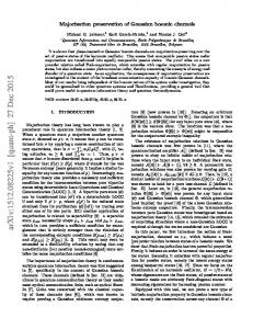
On the other hand, it is AD if a < 0 and N > N1 (see Fig. 2). Note that the defective Jordan blocks are not usually stable with respect to perturbations [20]. Indeed, we find numerically that, applying proper two-mode squeezing transformations to the environmental input, these weak-degradability conditions reduce to the decoupled case ones. In Fig. 1 we consider, for simplicity, a symmetric environmental initial state γE′ as in Eq. (105) with x = y, z− = 0 and ǫ = r, and we plot the relation between x, z+ and the minimum value of r such that J := J1 reduces to J := J0 corresponding to the decoupled case. One realizes that a squeezing parameter r close to 1 is enough to decouple the two modes representing the system, carrying quantum information. Moreover, let us point out that this squeezing threshold (r) increases slightly with the presence of correlations (z+ ) while decreases when increasing the level of noise (x) in the initial environmental state γE′ .

Figure 1: Relation between the parameters x, z+ and the minimum value of r in the initial environmental state such that the two-mode channel with X = 112 ⊕J1 reduces to the decoupled case X ′ = 112 ⊕ J0 with the same interaction parameter a for the two system modes. Finally, in the case of real Jordan block with complex eigenvalues, i.e., J2 as in Eq. (102), the corresponding two-mode bosonic Gaussian channels are WD if a > 1/2 and "  1/2 # 1 4b2 N > N2 := −1 + 1 + . (111) 2 (1 − 2a)2 while they are AD if a < 1/2 and N > N2 (see Fig. 2). In both of these cases (real and complex eigenvalues), in which the interaction term couples the two bosonic 26

Figure 2: In continuous line we report N1 as function of a in the case of J1 . For N > N1 the map is WD if a > 1 and AD if a < 0. In dashed line we plot N2 as function of b when a = 0 in the case of J2 . For N ≥ N2 the channel is WD (AD) if a > 1/2 (a < 1/2).

modes, there is the (apparently) counter-intuitive fact that above a certain environmental noise threshold the weak-degradability features appear, while for one-mode bosonic Gaussian channels they do not depend on the initial state of the environment. Actually, one would expect at most that, when the level of the environmental noise increases, the coherence progressively decreases until to be destroyed. It would mean that it becomes more and more difficult to recover the environment (system) output from the system (environment) output after the noisy evolution. However, the things go the other way around when multi-mode bosonic Gaussian channels are considered.

4.2 Channels with zero quantum capacity Analogously to Ref. [17] where the one-mode case is investigated, one can enlarge (other than the AD maps) the class of two-mode BGCs with Q = 0, composing a generic channel with an AD one. First of all, consider a channel Φ as in Section 2.3, but being AD (not necessarily minimal noise), then the maps Φ′ , defined in Eq. (63), have zero quantum capacity, i.e., they cannot be used to transfer quantum information. For instance, one can choose γE = (2Nc + 1)11n , i.e., the environmental initial state of the map Φ is a multi-mode thermal state with Nc being the average photon number for each mode, such that Φ is AD or simply with zero capacity; therefore, for any γE′ > γE = (2Nc + 1)11n , as in Eq. (65), the map Φ′ of Eq. (63) has Q = 0. Particularly for n = 2, using these observations and choosing Nc equal to either N1 (and a < 0) or N2 (and a < 1/2) as in Eqs. (110) and (111), one obtains that for X = 112 ⊕ J1,2 and Y ′ = s2 γE′ sT2 [with s2 as in Eq. (82)] the resulting channel Φ′ has always zero capacity. In this way, one extends considerably the set of two-modes maps with zero capacity, other than the very particular cases of two-mode 27

environmental thermal states studied above and shown in Fig. 2. For instance, twomode squeezing can be applied to the thermal state γE including not only states with N > Nc but also with not trivial two-mode correlations such that γE′ > (2Nc + 1)112 . Therefore, just considering this last simple inequality one includes so a larger set of maps that have zero quantum capacity. Moreover, we observe that, according to composition rules above, the combination Φ = ΦII ◦ ΦI of two channels ΦI and ΦII of class A2 and C, respectively, with Jordan blocks JI as in Eq. (100) with aI = bI and JII as in Eq. (102) with aII and bII 6= 0, gives J = aI JII which is in the class C. Now, since we have N1 > 0, N2 > 0 and assuming aI 6 1/2, the channel ΦI is AD and the resulting channel Φ must have Q = 0. Varying the parameters but keeping the product aI aII = a and aI bII = b fixed, the parameter N can assume any value satisfying the inequality " # 1/2 1 5(1 − 4a + 8a2 + 8b2 ) N > −2 . (112) 4 b2 + (a − 1)2 Note that aI has been chosen equal to 1/2 and ΦI corresponds to two uncoupled beam-splitter maps with transmissivity 1/2. We can therefore conclude that all channels of the form C with N as in Eq. (112) have zero quantum capacity – see Fig. 3. Consider now the composition Φ = ΦII ◦ ΦI of two channels ΦI and ΦII of class C and A2 (i.e., in the opposite order with respect to above), respectively, with Jordan blocks JI as in Eq. (102) with aI and bI 6= 0 and JII as in Eq. (100) with aII = bII , giving J = aII JI which is in the class C. As before, since we have N1 > 0, N2 > 0 and assuming again aII 6 1/2, the channel Φ2 is AD and the resulting channel has Q = 0. Varying the parameters but keeping the product aI aII = a and bI aII = b fixed, the parameter N can assume any value satisfying the inequality " # 1/2 (1 + 4a2 + 4b2 )(1 − 4a + 8a2 + 8b2 ) 1 −2 , (113) N > 4 4(b2 + (a − 1)2 )(a2 + b2 ) where again aII is chosen equal to 1/2. Again we can conclude that all class C channels with N as in Eq. (113) have zero quantum capacity. However, notice that the constraint in Eq. (113) is an improvement with respect to the constraint of Eq. (112) – see Fig. 3.

5 Conclusions In this work, we have presented a complete analysis of generic multi-mode Gaussian channels by proving a unitary dilation theorem and by finding their canonical form. This is a simple form that can be achieved for any Gaussian quantum channel, as a convenient starting point for various considerations. For instance, it allows us to simplify the analysis of the weak-degradability properties of multi-mode bosonic Gaussian channels. Minimal output entropies, or quantum and classical information capacities and other difficult questions might be tackled using the canonical form of multi-mode Gaussian channels shown in this paper. Here, we investigated in details 28

Figure 3: The continuous line depicts plot N2 as in Eq. (111) versus b, with a = 1 in J2 of Eq. (102). For N ≥ N2 the channel is WD (AD) if a > 1/2 (a < 1/2). The dashed line refers to the bound in Eq. (112), while the dashed-dot line to the one in Eq. (113); above these bounds the class C map is WD but with Q = 0. Note that Eq. (113) is an improvement with respect to the constraint of Eq. (112). Similar bounds can be obtained in the case a < 1/2, enlarging the group of AD maps with other channels with Q = 0.

the two-mode scenario that is relevant since any n-mode channel can always be reduced to single-mode and two-mode parts [20]. Furthermore, the results of this paper could play a basic role in characterizing the efficiency of continuous-variables quantum information processing, quantum communication and quantum key distribution protocols.

6 Acknowledgements F.C. and V.G. thank the Quantum Information research program of Centro di Ricerca Matematica Ennio De Giorgi of Scuola Normale Superiore for financial support. J.E. acknowledges the EPSRC, the QIP-IRC, the EU (QAP, COMPAS), Microsoft Research, and the EURYI Award Scheme for financial support. A.S.H. acknowledges support of RFBR grant 06-01-00164-a and the RAS program “Modern problems of theoretical mathematics”.

A Proof of Lemma 1 E Note that it does not restrict generality to take σ2ℓ = σ2ℓ , as this can always be accompanied by an appropriate similarity transform. Our problem at hand of extending a symplectic form is then equivalent to the following problem: Suppose we are given

29

column vectors e1 , · · · , en and f1 , · · · , fn from

R2(n+ℓ) that satisfy

eTj σ2(n+ℓ) ek = 0,

(114)

fjT σ2(n+ℓ) fk eTj σ2(n+ℓ) fk

= 0,

(115)

= δj,k ,

(116)

for j, k = 1, · · · , n. The procedure continues by identifying vectors en+1 and fn+1 such that eTn+1 σ2(n+ℓ) fn+1 = 1 and T eTn+1 σ2(n+ℓ) w = fn+1 σ2(n+ℓ) w = 0

(117)

w ∈ Wn := span(e1 , · · · , en , f1 , · · · , fn ).

(118)

for all Now define Wn⊥ = {w : w T σ2(n+ℓ) v = 0 ∀v ∈ Wn }.

R

2(n+ℓ)

Wn ∩ Wn⊥

(119) Wn ⊕ Wn⊥ :

= Suppose It is now not difficult to see that = {0} and that the vector v has v T σ2(n+ℓ) ej =: αj and v T σ2(n+ℓ) fj =: βj for j = 1, · · · , n. Then " n # " # n X X v= (−αj fj + βj ej ) + v + (αj fj − βj ej ) , (120) j=1

j=1

where the first term is element of Wn and the second of Wn⊥ . Following a symplectic Gram-Schmidt procedure, the symplectic basis can hence be completed, which is equivalent to extending the matrices s1 and s2 to a symplectic   s1 s2 (121) ∈ Sp(2(n + ℓ), ). S= s3 s4

R

B Derivation of Eq. (35) Here we show that Eq. (35) admits solution for s′2 as in Eq. (41). In fact, assuming E σ4n = σ2n ⊕ σ2n with σ2n as in Eq. (1), one has    −T   −1  σ2n 0 K ′ E ′ T ′ T K O A s2 σ4n (s2 ) − Σ = − Σ′ 0 σ2n AT O = K −1 σ2n K −T + O T A σ2n AT O − Σ′
= K −1 KΣ′ K T + B K −T + O T A σ2n AT O − Σ′ = K −1 BK −T + O T A σ2n AT O
= O M 1/2 BM 1/2 + A σ2n AT O T ,

(122)

where we used Eq. (40) to write σ2n = KΣ′ K T + B, with B being the 2n × 2n matrix   0 0 0  0 11n−r/2  . (123) B :=    0 0 0 0 −11n−r/2

The identity (35) finally follows by noticing that the last term in Eq. (122) cancels since M 1/2 B = BM 1/2 = B and A σ2n AT = −B. 30

C Properties of the environmental states In this appendix we first give an explicit derivation of Eq. (43). Then we analyze in details the property of the state ρˆE associated with the covariance matrix γE defined be the Eqs. (45) and (46). Replacing Eq. (41) into Eq. (26), we get    −T   α δ  −1 K ′ ′ T T O A K 112n = s2 γE (s2 ) = T δ β AT O

which leads to

= K −1 α K −T + O T A δ T K −T + K −1 δ AT O + O T A β AT O
= O T M 1/2 α M 1/2 + A δ T M 1/2 + M 1/2 δ AT + A β AT O ,

M −1 = α + M −1/2 A δ T + δ AT M −1/2 + M −1/2 A β AT M −1/2 ,

(124)

and hence to Eq. (43) by the fact M −1/2 A = AT M −1/2 = A = AT . Such an equation admits the solution given in Eqs. (45) and (46). Explicitly this corresponds to the 4n × 4n covariance matrix γE of the form   0 f (µ−1) 0 µ−1 0 0  0 ξ 11 0 f (ξ 11)    −1 −1   µ 0 f (µ ) 0   0 0   0 ξ 11 0 f (ξ 11)   −1 −1   f (µ ) 0 µ 0   0 0   0 f (ξ 1 1) 0 ξ 1 1   −1   f (µ−1 ) 0 µ 0 0 0 0 f (ξ 11) 0 ξ 11

where for easy of notation 11 := 11n−r/2 . By looking at the structure of this covariance matrix, one realizes that it is composed by two independent sets formed by r and 2n − r modes, respectively. The first set describes r/2 thermal states characterized by the matrices µ−1 which have been purified adding further r/2 modes. The second set instead describes a collection of 2(n − r/2) = 2n − r modes prepared in a pure state formed by n − r/2 independent pairs of modes which are entangled. By reorganizing its rows and columns this can be cast into the simpler form   µ ¯−1 f (¯ µ−1) }r 0 −1 −1  f (¯  }r µ ) µ ¯  γE =  (125)  ξ 112n−r f (ξ 112n−r )  } 2n − r 0 } 2n − r , f (ξ 112n−r ) ξ 112n−r where we used µ ¯ to indicate the r × r matrix µ ¯ = µ ⊕ µ.

C.1

Solution for ℓpure = 2n − r′ /2 environmental modes

Defining r ′ as in Eq. (57) we choose the environmental commutation matrix to be E σ2ℓ = σ2n ⊕ σ2n−r′ with σ2n and σ2n−r′ as in Eq. (1). A unitary dilation with ℓpure = 31

2n−r ′ /2 environmental modes in a pure state is obtained by having s2 = Y 1/2 s′2 with s′2 as in Eq. (41). In this case, however, A is a rectangular matrix 2n × 2(n − r ′ /2) of the form   0 0 } r ′ /2  } (r − r ′ )/2  0 0 0    0 11n−r/2   } n′ − r/2  (126) A =   } r /2 0 0    } (r − r ′ )/2  0 0 0 } n − r/2. 0 11n−r/2

Similarly, the covariance matrix γE can be still expressed as in Eq. (44). In this case, yet, α is a 2n × 2n matrix of block form   11r′ /2 0 0 } r ′/2 −1  } (r − r ′ )/2  0 µo 0 0    } n − r/2  0 0 ξ 11n−r/2   (127) α=  } r ′/2 ′ /2 1 1 0 0 r    } (r − r ′ )/2  0 µ−1 0 0 o } n − r/2, 0 0 ξ 11n−r/2

where ξ = 5/4 and µo is the (r − r ′ )/2 × (r − r ′ )/2 diagonal matrix formed by the elements of µ which are strictly smaller than 1. β is the (2n − r ′ ) × (2n − r ′ ) matrix   µ−1 0 } (r − r ′ )/2 o 0   } n − r/2 0 ξ 11n−r/2  β= (128) −1   } (r − r ′ )/2 µo 0 0 } n − r/2, 0 ξ 11n−r/2 and



   δ=   

0 f (µ−1 o ) 0

0 0 f (µ−1 o ) 0

0 0 f (ξ 11n−r/2 )

0 0 f (ξ 11n−r/2 ) 0

       

} r ′ /2 } (r − r ′ )/2 } n − r/2 (129) } r ′ /2 } (r − r ′ )/2 } n − r/2,

with f as in Eq. (46). By looking at the structure of this covariance matrix, one realizes that it is composed by three independent pieces. The first one describes a collection of r ′ /2 vacuum states. The second one, in turn, describes (r − r ′ )/2 thermal states characterized ′ by the matrices µ−1 o which have been purified by adding further (r − r )/2 modes. The third one, finally, reflects a collection of 2(n − r/2) = 2n − r modes prepared in a pure state formed by n − r/2 independent pairs of modes which are entangled.

32

C.2

Solution for ℓ = 2n − r/2 not necessarily pure environmental modes

In this subsection, we present the alternative derivation of a dilation that does not necessarily involve an environment prepared in a pure state. Choosing the commuE tation matrix σ2ℓ = σ2n ⊕ σ2n−r with σ2n and σ2n−r as in Eq. (1), the matrix s′2 can be still expressed as in Eq. (41). In this case, however, A is a rectangular matrix 2n × (2n − r) of the form   0 } r/2 0   11n−r/2  } n − r/2 . (130) A =   } r/2  0 0 } n − r/2, 11n−r/2

Similarly, γE has the block form (44), where α is still the 2n × 2n matrix of Eq. (45), while β and δ are, respectively, the following (2n − r) × (2n − r) and 2n × (2n − r) real matrices:   0 ξ 11n−r/2 } n − r/2 β= (131) } n − r/2, 0 ξ 11n−r/2  0 0 } r/2   0 f (ξ 11n−r/2 )  } n − r/2 δ=  } r/2  0 0 } n − r/2, f (ξ 11n−r/2 ) 0 

with ξ and f as in Eq. (46). That is,  µ−1 0 0  0 ξ 11   µ−1 0 0 γE =   0 ξ 11   0 0 0 f (ξ 11) 0 f (ξ 11) 0 0

0 0 0 f (ξ 11) ξ 11 0

0 f (ξ 11) 0 0 0 ξ 11

(132)

       

} r/2 } n − r/2 } r/2 (133) } n − r/2 } n − r/2 } n − r/2 ,

with 11 = 11n−r/2 . This covariance matrix now consists of two independent parts: The first one describes a collection of r/2 thermal states described by the matrices µ−1 . The second instead reflects a collection of 2(n − r/2) = 2n − r modes prepared in a pure state formed by n−r/2 independent couples of modes which are entangled. The covariance matrix given in Theorem 1 can be recovered from the one given above by adding r modes to purify the thermal states µ−1 .

D Equivalent unitary dilations Let S=



s1 s2 s3 s4 33



(134)

and γE define a unitary dilation for a bosonic Gaussian channel Φ characterized by matrices X and Y . Then a full class of unitary dilations  ′  s1 s′2 ′ S = (135) s′3 s′4 can be obtained by taking γE′ = V γE V T and s′1 = s1 ,

s′2 = s2 V

R

s′3 = W s3 ,

s′4 = W s4 V ,

(136)

R

with V ∈ Sp(2ℓ, ) and W ∈ Sp(2n, ) being symplectic transformations of ℓ and n modes respectively. With this choice in fact γE′ is still a covariance matrix while the conditions (23) and (24) are automatically satisfied. From a physical point of view the symplectic transformations V and W correspond to unitary local operations applied to the environmental input and output states, respectively, by virtue of the ˜ and metaplectic representation. Consequently, the weak complementary channels Φ ′ ˜ associated with these two representations are unitarily equivalent and the weakΦ degradability properties one can determine for Φ will be the same when studied for Φ′ . Conversely, let us suppose to have two unitary dilations of Φ, realized with ℓ = n environmental modes and characterized by the symplectic matrices S and S ′ as in Eq. (134) and (135), respectively, with si and s′i being 2n × 2n square matrices. Then it is possible to show that they must be related as in Eq. (136) under the hypothesis that s2 and s3 are non-singular. First of all, since Eq. (24) must be satisfied for all the ′ input covariance matrices γ, we have s1 = X T = s′1 . Define then V = s−1 2 s2 and W = s′3 s−1 3 . By using the first of Eq. (23) and exploiting the non-singularity of s2 one has E V T sT2 = s2 σ2n sT2 s2 V σ2ℓ

=⇒

V σ2n V T = σ2n ,

(137)

E which implies that V is a symplectic matrix (we are assuming σ2ℓ = σ2n ). Moreover, ′ from the second condition in Eqs. (23) for S and S , we obtain

s2 σsT4 W T = s2 V σs′T 4 ,

=⇒

s′4 = W s4 V ,

(138)

because s2 is non-singular and V is symplectic. By considering the third condition (23) one then has W (s3 σ2n sT3 + s4 σ2n sT4 )W T = W σ2n W T = σ2n

(139)

which prove that W is a symplectic. Finally, let us observe that the proof above does not use the non-singularity of s3 . Indeed, one can relax this hypothesis and assume more simply that there exists a W such that s′3 = W s3 ; from Eqs. (23) W has to still be a symplectic matrix but s3 and s′3 may be singular. As an application of these equivalent unitary dilation results, we can find an alternative canonical form to the one in Sec. 2.5 with the same s1 and s4 but with s2 and s3 of the following anti-diagonal block form   0 Fj (140) sj = Gj 0 34

where, for j = 2, 3, Fj , Gj are n × n real matrices. Imposing Eqs. (23), one obtains the following relations J T − F2 GT2 = 11n , J ′T − F3 GT3 = 11n , F2 − F3T = 0 , JGT3 − G2 J ′T = 0 , the solution of which provides the following unitary dilation,  11n 0 0 −(11n − J T )G−T 2  0 J G 0 2 S=  0 −G−1 0 2 (11n − J) 11n T T −T T 0 G2 J G2 G2 0

(141)



 , 

(142)

where again G2 is an arbitrary (non-singular) matrix and the eigenvalues of J are assumed to be different from 1. This solution is unitarily equivalent to the one in Eq. (79) by applying V = −σ2n and   −1 0 G−1 G2 2 J W = (143) −GT2 J T G−T 0 2 as above.

E The ideal-like quantum channel Here we consider a quantum channel with X = 112n but Y > 0 with rank less than 2n, which can be described in terms of only n additional (environmental) modes. We call it ideal-like quantum channel. Accordingly, the canonical unitary transformation Uˆ of Eq. (20) will be uniquely determined by a 4n × 4n real matrix S ∈ Sp(4n, ) of block form in Eq. (22), where si are 2n × 2n real matrices. Particularly, s1 = s4 = 112n ,     −GT3 0 F3 0 , (144) , s2 = s3 = 0 −F3T 0 G3

R

with F3 and G3 being n × n real matrices such that F3 GT3 = GT3 F3 = 0, in order to satisfy the symplectic conditions in Eqs. (23). Taking advantage of the freedom in the choice of the unitary dilation shown in Appendix D, the matrix S can be put in the form of Eq. (22) in which s′1 = s′4 = 112n ,     0 0 −11n 0 ′ ′ s2 = , s3 = , (145) 0 11n 0 0

R

where F3 is assumed non-singular. In this respect, one uses V, W ∈ Sp(2n, ) (of App. D) of the following form   −F3 0 V = , (146) 0 −F3−T and W = V −1 . Similarly, one can proceed, if G3 is non-singular, and obtains a similar structure for S as above. As concerns the weak-degradability properties, if 35

one assumes the initial environmental input state as γE = diag(2N +1, 2M +1, 2N + ˜ T X −T (Y + iσ)X −1 X ˜ + iσ are {2M, 2(M + 1, 2M + 1), the eigenvalues of Y˜ − X 1), 2N, 2(N + 1)}, which are always positive for any N > 0 and M > 0; hence, this channel with γE as above is always weakly degradable. Finally, one may consider Nnanother ideal-like channel with X = 112n and Y = ⊗n [(1−σ3 )/4] , i.e. ΦX,Y = i=1 (B1 )i , where the single-mode B1 channel is defined in Ref. [17] as X = 112 and Y = (1 − σ3 )/4. Trivially, this multi-mode channel is always WD (like B1 ) and is able to transfer a quantum state without decoherence with the maximum quantum capacity (like for the single-mode case [17]).

References [1] A.S. Holevo, Probabilistic and Statistical Aspects of Quantum Theory (Amsterdam: North-Holland, 1982). [2] A.S. Holevo, M. Sohma, and O. Hirota, Phys. Rev. A 59, 1820 (1999). [3] A.S. Holevo and R.F. Werner, Phys. Rev. A 63, 032312 (2001). [4] J. Eisert and M.M. Wolf, arXiv:quant-ph/0505151. [5] A.S. Holevo, Probl. Inf. Transmission 8, 1 (1972). [6] B. Demoen, P. Vanheuswijn, and A. Verbeure, Lett. Math. Phys. 2, 161 (1977). [7] A. Ferraro, S. Olivares, and M.G.A. Paris, Gaussian States in Quantum Information (Napoli: Bibliopolis, 2005). [8] S.L. Braunstein and P. van Loock, Rev. Mod. Phys. 77, 513 (2005). [9] C.M. Caves and P.D. Drummond, Rev. Mod. Phys. 66, 481 (1994). [10] M. Navasu´es, F. Grosshans, and A. Ac´ın, Phys. Rev. Lett. 97, 190502 (2006); R. Garcia-Patr´on and N.J. Cerf, Phys. Rev. Lett. 97, 190503 (2006). [11] V. Giovannetti, S. Lloyd, L. Maccone, J.H. Shapiro, and B.J. Yen, Phys. Rev. A 70, 022328 (2004). [12] V. Giovannetti, S. Guha, S. Lloyd, L. Maccone, J.H. Shapiro, and H.P. Yuen, Phys. Rev. Lett. 92, 027902 (2004). [13] A. Serafini, J. Eisert, and M.M. Wolf, Phys. Rev. A 71, 012320 (2005). [14] A.S. Holevo, Probl. Inf. Transm. 43, 1 (2007). [15] M.M. Wolf, D. Perez-Garcia, and G. Giedke, Phys. Rev. Lett. 98, 130501 (2007) [16] F. Caruso and V. Giovannetti, Phys. Rev. A 74, 062307 (2006). [17] F. Caruso, V. Giovannetti, and A.S. Holevo, New J. Phys. 8, 310 (2006). 36

[18] G. Lindblad, J. Phys. A 33, 5059 (2000). [19] S. Lloyd, Phys. Rev. A 55, 1613 (1997); H. Barnum, M.A. Nielsen, and B. Schumacher, Phys. Rev. A 57, 4153 (1998); I. Devetak, IEEE Trans. Inf. Theory, 51, 44 (2005). [20] M.M. Wolf, Phys. Rev. Lett. 100, 070505 (2008). [21] J. Eisert and M.B. Plenio, Int. J. Quant. Inf. 1, 479 (2003). [22] G. Adesso and F. Illuminati, J. Phys. A 40, 7821 (2007). [23] J. Williamson, Am. J. Math 58, 141 (1936); Am. J. Math 59, 599 (1937); 61, 897 (1939). [24] W.F. Stinespring, Proc. Am. Math. Soc. 6, 211 (1955). [25] A. Cannas da Silva, Lectures on Symplectic Geometry (LNM, Springer, 2001). [26] R.A. Horn and C.R. Johnson, Matrix Analysis (Cambridge University Press, Cambridge, 1990). [27] I. Devetak and P.W. Shor, Commun. Math. Phys. 256, 287 (2005). [28] A.S. Holevo, Theory Probab. Appl. 51, 133 (2005). [29] C. King, K. Matsumoto, M. Nathanson, and M.B. Ruskai, Markov Processes and Related Fields, special issue in memory of John T. Lewis, Vol. 13, Issue 1, pp. 391-423 (2007). [30] G. Lindblad, Commun. Math. Phys. 48, 116 (1976). [31] J. Eisert, S. Scheel, and M.B. Plenio, Phys. Rev. Lett. 89, 137903 (2002); J. Fiurasek, Phys. Rev. Lett. 89, 137904 (2002); G. Giedke and J.I. Cirac, Phys. Rev. A 66, 032316 (2002); G. Giedke, J. Eisert, J.I. Cirac, and M.B. Plenio, Quant. Inf. Comp. 3, 211 (2003). [32] J. Laurat et al., J. Opt. B 7, S577 (2005).

37