their networks, Internet multicast is only widely available as an overlay service, known as the Mbone [7]. Commercial overlay networks, such as Akamai [1] and ...
1
Multicast Routing and Bandwidth Dimensioning in Overlay Networks Sherlia Y. Shi Jonathan S. Turner Department of Computer Science Washington University in St. Louis {sherlia, jst}@cs.wustl.edu Abstract Multicast services can be provided either as a basic network service or as an application-layer service. Higher level multicast implementations often provide more sophisticated features, and can provide multicast services at places where no network layer support is available. Overlay multicast networks offer an intermediate option, potentially combining the flexibility and advanced features of application layer multicast with the greater efficiency of network layer multicast. In this paper, we introduce the multicast routing problem specific to the overlay network environment and the related capacity assignment problem for overlay network planning. Our main contributions are the design of several routing algorithms that optimize the end-to-end delay and the interface bandwidth usage at the multicast service nodes within the overlay network. The interface bandwidth is typically a key resource for an overlay network provider, and needs to be carefully managed in order to maximize the number of users that can be served. Through simulations, we evaluate the performance of these algorithms under various traffic conditions and on various network topologies. The results show that our approach is cost-effective and robust under traffic variations. Keywords Overlay networks, load-balancing routing, multicast routing, network planning
I. I NTRODUCTION Multicast communication is an important part of many next generation networked applications, including video conferencing, video-on-demand, distributed interactive simulation (including large multi-player games) and peer-to-peer file sharing. Multicast services allow one host to send information to a large number of receivers, without being constrained by its network interface bandwidth. This makes applications more scalable and leads to more efficient use of network resources. However, the limited network layer support for multicast in the Internet today, has made it necessary for applications requiring multicast services to obtain services at a higher level. In application layer multicast, hosts participating in an application session share responsibility for forwarding information to other hosts [9, 16, 18, 20, 26]. While highly flexible, this approach places a significant additional burden on hosts, and is not as efficient as networklayer multicast. Overlay multicast networks effectively use the Internet as a lower level infrastructure, to provide higher level services to end users. It provides multicast services through a set of distributed Multicast Service Nodes (MSN), which communicate with hosts and with each other using standard unicast mechanisms. Overlay multicast networks play an important role in the Internet. Indeed, since Internet Service Providers have been slow to enable IP multicast in their networks, Internet multicast is only widely available as an overlay service, known as the Mbone [7]. Commercial overlay networks, such as Akamai [1] and iBeam [17], also use overlay multicast to improve their network efficiencies.
2
Because overlay multicast networks are built on top of a general Internet unicast infrastructure rather than point-topoint links, the problem of managing their resource usage is somewhat different than in networks that do have their own links, leading to differences in how they are best configured and operated. These main differences are: •
Network reachability: The overlay network is a fully meshed network, as each node is able to reach everybody else
in the network via unicast connections. Therefore, unlike in IP multicast where a path from one router to another is defined by its physical connectivity, an n-node overlay multicast session could have n n−2 different spanning trees [4], leading to a larger design space and more design complexity. •
Network cost: Historically, the cost of a network is determined largely by the summation of individual link costs.
This is certainly true for network providers who have to physically deploy the links or lease them from others. But from an application service provider’s point of view, the cost associated with provisioning an overlay network is the total amount paid to gain access bandwidth at each server site to the backbone network. This divergence of cost metric has a deep impact on both design and routing strategies in overlay networks. •
Routing constraints: Traditional IP multicast routes through a shortest path tree to minimize delay from source to
all receivers, i.e. reducing the number of links needed to carry session traffic. Building the network at the service level gives the flexibility of matching routing strategies to application needs. For applications such as streaming media or conferencing, a routing strategy that produces bounded delay between any pair of participants results in significantly higher quality from an application’s perspective. In this paper, we address two problems. First, given a set of MSN locations and a set of traffic assumptions, we want to find an assignment of network access bandwidth to each MSN site, subject to a fixed overall bandwidth constraint; we refer to this procedure as the dimensioning process. Second, given the above dimensioned network, we want to devise routing algorithms that dynamically route multicast sessions and make the best use of the available network resources so as to accommodate the maximum number of sessions, as well as satisfying an application delay constraint. The two problems interact. Knowledge of the routing algorithm allows the dimensioning process to allocate bandwidth to the MSNs in a way that best serves the routing algorithm’s needs. On the other hand, the performance of a routing algorithm is significantly affected by the difference between the bandwidth assignment in the underlying network and the actual traffic load. Using simulation, we show that by using routing algorithms that seek to balance the access bandwidth usage at each MSN’s interface, we can achieve high network utilization with low session rejection rate. The rest of the paper is organized as follows: in section II, we detail our design objectives and problem definitions; In section III and IV, we introduce the routing algorithms and the dimensioning process, respectively; In section V, we evaluate the performance of the routing algorithms on different network topologies and under various traffic conditions; In section VI, we introduce a hybrid scheme to reduce the routing complexity; In section VII, we discuss some of the related work and we conclude in section VIII.
3
II. D ESIGN O BJECTIVES AND P ROBLEM D EFINITIONS One of the principal resources that an overlay network must manage is the access bandwidth to the Internet at the MSNs’ interfaces. This interface bandwidth represents a major cost, and is typically the resource that constrains the number of simultaneous multicast sessions that an overlay network can support. Hence, the routing algorithms used by an overlay multicast network, should seek to optimize its use. Additionally, a multicast routing algorithm should ensure that the routes selected for multicast sessions do not contain excessively long paths, as such paths can lead to excessively long packet delays. However, the objective of limiting delay in a multicast network can conflict with the objective of optimizing the interface bandwidth usage, so multicast routing algorithms must strike an appropriate balance between these two objectives. An overlay multicast network can be modeled as a complete graph since there exists a unicast path between each pair of MSNs. For each multicast session, we create a shared overlay multicast tree spanning all MSNs serving participants of a session, with each tree edge corresponding to a unicast path in the underlying physical network. The degree of an MSN node in the multicast tree represents the amount of access bandwidth in use to support the multicast session and the total amount of available interface bandwidth at an MSN imposes a constraint on the maximum degree of that node in the multicast tree. We let dmax (v) denote this degree constraint at node v. There are two natural formulations of the overlay multicast routing problem: the first seeks to minimize the multicast tree diameter while respecting the degree constraints at individual nodes; and the other optimizes on the degree distribution among session nodes with respect to their current available interface bandwidth while satisfying an upper bound on the tree diameter. We formalize the problems as follows. Definition 1: Minimum diameter, degree-limited spanning tree problem (MDDL ) Given an undirected complete graph G = (V, E), a degree bound d max (v) ∈ N for each vertex v ∈ V and a cost c(e) ∈ Z + for each edge e ∈ E; find a spanning tree T of G of minimum diameter, subject to the constraint that dT (v) ≤ dmax (v) for all v ∈ T . Much previous research has been done on related problems. In [13], Ho et al. proved that in geometric space, there exists a minimum diameter spanning tree in which there are at most two interior points (non-leaf nodes) and the optimal tree can be found in O(n3 ) time. Hassin and Tamir established in [12], that for a general graph, a minimum diameter spanning tree problem is identical to the absolute 1-center problem introduced by Hakimi [11] and as such, a solution can be found in O(mn + n2 logn), where n is the number of nodes and m the number of edges. In [13] and [21] respectively, they prove that minimum diameter, minimum spanning tree and minimum maximum degree, minimum spanning tree are both NP-complete. Theorem 1: The decision version of MDDL– finding a spanning tree with diameter bound B and a degree constraint dmax (v) for each node, is NP-complete, for 2 ≤ dmax (v) ≤ |V | − 1. Proof:
Clearly, the problem is in NP, since we can verify in polynomial time if a candidate solution satisfies both
4
the diameter and degree constraints. For the special case where d max (v) = 2 for all v ∈ V , the problem is the same as the path version of the Traveling Salesman Problem (TSP) [10]. We reduce from the TSP problem for the general case of dmax (v) ≥ 2. Let G = (V, E) be the graph of a TSP instance. We transform G to G 0 = (V 0 , E 0 ) by adding dmax (v) − 2 vertices u1 , . . . , udmax (v)−2 to each v ∈ V . We join each of these new vertices ui to v with edges of zero length; All other edges from ui have length B + 1, so that G0 is still a complete graph. Now, the MDDL instance in G0 has a spanning tree of diameter B if and only if the TSP instance has a path of length B that includes all the vertices in G. For the case that all nodes have dmax (v) ≥ |V |−1, or in other words there are no constraint on the nodes’ degree since the maximum possible degree for any node in a tree is |V | − 1, the problem is polynomial solvable. More specifically, a minimum diameter tree can be found as the shortest path tree with the smallest diameter, among all shortest path trees rooted at each node. The second formulation of the overlay multicast routing problem seeks the “most balanced” tree, that satisfies an upper bound on the diameter. To explain what is meant by “most balanced”, we first define the residual degree at node v with respect to a tree T as resT (v) = dmax (v) − dT (v), where dT (v) is the degree of v in T . To reduce the likelihood of blocking a future multicast session request, we should choose trees that maximize the smallest residual degree. Since the sum of the degrees of all multicast trees is the same, this strategy works to “balance” the residual degrees of different vertices. Any tree that maximizes the smallest residual degree is a “most balanced” tree. Definition 2: Limited diameter, residual-balanced spanning tree problem (LDRB) Given an undirected complete graph G = (V, E), a degree bound d max (v) for each v ∈ V , a cost c(e) ∈ Z + for each e ∈ E and a bound B ∈ Z + ; find a spanning tree T of G with diameter ≤ B that maximizes minv∈V resT (v), subject to the constraint that dT (v) ≤ dmax (v), for all v ∈ V . This problem is also NP-complete, since the special case in which every node has a degree of two, corresponds to the decision version of the TSP problem. III. M ULTICAST ROUTING A LGORITHMS In overlay multicast routing, we assume that there is a designated MSN for each session to compute the multicast tree. The designated MSN has full knowledge of other MSNs in the session, and computes the multicast tree according to its current snapshot of the available bandwidth at these MSNs. The state updates occur periodically via broadcasting among all MSNs. For the purpose of this paper, we will assume that the designated MSN always has the most up-todate information regarding to other MSNs, although in practice, it is likely that the updates will occur less frequently than the session requests and that the routing performance may be deterred due to the imprecise routing information. Interested readers are referred to [23] for an examination of the trade-off between the frequency of updates and the routing performance. The choice of the centralized route computation is to increase routing efficiency and reduce message complexity by
5
eliminating the many message exchanges required to coordinate a distributed computation. We should point out that the centralized version does not create a single point of failure or even a performance bottleneck, as each session may select a different delegate to perform the tree computation. During periods of heavy network load, we can expect there to be lots of session routing computations being performed concurrently. This means that the overall computational load can be effectively distributed by having different MSNs do the computation for different sessions. We believe that the greater efficiency of this approach, relative to a distributed routing computation for each session, will more than compensate for any inequities in the load distribution that are likely to arise in practice. In this section, we first present two greedy heuristic algorithms for the MDDL and LDRB problems; then we introduce a new algorithmic strategy for the
LDRB
problem that takes a more direct approach to optimizing the MSN interface
bandwidth. Based on the second approach, we describe several specific tree-building techniques. These algorithms are evaluated using simulation in section V. A. The Compact Tree Algorithm The Compact Tree (CT) algorithm for the
MDDL
problem is a greedy algorithm, which like Prim’s algorithm for
Minimum Spanning Tree [6], builds a spanning tree incrementally. For each vertex u in the partial spanning tree T , constructed so far, let δ(u) denote the length of the longest path from vertex u to any other node in T . For each vertex v that is not yet in the partial tree T constructed so far, we maintain an edge λ(v) = {u, v} to a vertex u in the tree; u is chosen to minimize δ(v) = c(λ(v)) + δ(u). At each step, we select a vertex v with the smallest value of δ(v) and add it and the edge λ(v) to the tree. Then, for each vertex v, not yet in the tree, we update λ(v). This process is repeated for each vertex. Figure 1 gives a detailed description. The algorithm fails when it finishes with some vertices having δ(v) = ∞, meaning that we cannot build a spanning tree with the specified set of degree constraints. There are two cases for this to happen: one is that a session request may arrive at a set of MSNs whose total available bandwidth (the sum of the degree constraints) is less than the minimum required degree, 2 ∗ (|V | − 1), for a session spanning tree. In this case, the session request is simply rejected; The other case is that during the progression of the algorithm, a vertex with a degree constraint of one is added to the tree, when the sum of the spare degrees of the tree vertices is also one. Such addition leaves the newly formed tree component with zero spare degree and we cannot add any more nodes to the tree. To remedy this, we add a count of the spare degrees of the tree component and defer the addition of a leaf node if it reduces the count to zero. It is known that the TSP problem on a graph is MAX-SN P-hard [14]. Since TSP is a special case for the problem when all nodes’ degree constraints are equal to two, the
MDDL
MDDL
problem therefore cannot be approximated to
within some constant factor unless P = N P . At this time, we do not know the approximability of the MDDL problem in general. The CT algorithm, on the other hand, gives an O(log n) approximation ratio as shown by the following proof. Let λGreedy and λ∗ denote the tree diameter constructed by the greedy algorithm and an optimal solution, respectively. And let dmin = min(dmax (u)) and dmax = max(dmax (u)).
6
Input: G = (V, E) Edge cost c(u,v), for u, v ∈ V Degree constraints dmax (v) Output: tree T foreach r ∈ V do foreach v ∈ V do δ(v) = c(r, v); λ(v) = {r, v}; T = (W={r}, L={}); while (W 6= V ) do let u ∈SV − W be S the vertex with smallest δ(u); W = W {u}; L = L {λ(u)}; foreach v ∈ W − {u} do δ(v) = max{δ(v), distT (u, v)}; foreach v ∈ V − W do δ(v) = ∞; foreach q ∈ W do if degree(q) < dmax (q) and c(v, q) + δ(q) < δ(v) then δ(v) = c(v, q) + δ(q); λ(v) = {v, q}; Fig. 1. The CT Heuristic Algorithm for MDDL
Lemma 1: If the ratio of edge weights is bounded by ε ∈ Z + , and the degree constraints satisfy 2 < dmin ≤ dmax < |V | − 1, then λGreedy < O(k)λ∗ , where k = ε logdmin dmax . Proof: Without loss of generality, let the smallest edge weight be 1 and the largest edge weight ε. The optimal solution achieves λ∗ > 2 logdmax n. Now, let’s assume a simple algorithm A for constructing a spanning tree: at each step of adding a new node, A simply selects a node to maximize the degree of u ∈ T without consideration of the tree diameter. In the worst case, λA < 2ε(logdmin n). We observe that λGreedy ≤ λA , since when adding a new node, the greedy algorithm always attempts to select the one node which will result in the smallest diameter increase. Therefore, λGreedy < kλ∗ , where k = ε logdmin dmax . B. The Balanced Compact Tree Algorithm The Balanced Compact Tree (BCT) algorithm is a heuristic for the
LDRB
problem and can be viewed as a general-
ization of the CT algorithm. Like the CT algorithm, it builds the tree incrementally. However, at each step it first finds the M vertices that have the smallest values of δ(v) and from this set, it selects a vertex v with λ(v) = {u, v}, that maximizes the smaller of resT (u) and resT (v), where T is the current partial tree. The parameter M may be varied to trade-off the goals of residual degree balancing and diameter minimization. Specifically, when M = 1, it is equivalent to the CT algorithm; and when M is equal to the number of vertices in the multicast session, BCT concentrates on balancing the residual degrees. Simulation studies have shown that fairly small values of M are effective in achieving good balance, without violating the diameter bound. We evaluate overlay multicast routing algorithms using a simulation in which new multicast sessions are dynamically
7
generated as a Poisson process. The primary performance metric is the fraction of sessions that are rejected because no multicast route can be found, either due to the failure to satisfy the diameter bound or due to the exhaustion of interface bandwidth of at least one MSN. We also obtain a lower bound on the rejection probability using a simulation in which a multicast session is rejected only if the MSN interface bandwidth required by the session exceeds the total unused interface bandwidth at all MSNs (including those not involved in the session). Results in section V show that by distributing the load more evenly across servers, the BCT algorithm rejects substantially fewer multicast sessions than the CT algorithm on the same network configuration. At the mean time, there remained a significant gap between the achieved performance and the potential suggested by the lower bound. While the bound was not expected to be tight, the size of the gap suggested that there was room for improvement. In the next subsection, we introduce a new strategy for overlay multicast routing that leads to an algorithm with uniformly better performance. C. Balanced Degree Allocation In the BCT algorithm, a new node is always attached to the tree at the point that yields the smallest diameter in the resulting tree. Although the algorithm changes the sequence of node selection by first selecting nodes with larger residual degrees, it does not guarantee the use of these nodes as intermediate nodes in the tree, i.e. nodes with higher degree fanout. This prevents the BCT algorithm from achieving the best-possible residual degree balance. Balanced Degree Allocation (BDA) is a strategy for constructing multicast trees that approaches the problem in a fundamentally different way. It starts by determining the ideal degree of each node in the multicast session, with respect to the objective of maximizing the smallest residual degree. To state the strategy precisely, we need to stretch our definition of the residual degree of a vertex. Let k denote the multicast session size (or interchangeably session fanout). First, we define a degree allocation d A to be a function from the vertices of a multicast session to the positive integers that satisfies two properties: (1)
P
v
dA (v) = 2(k − 1),
where k is the number of participants in the multicast session (so, 2(k − 1) is the sum of the vertex degrees in any tree implementing the multicast session); and (2) there are at least two vertices u and v with d A (u) = dA (v) = 1. A partial degree allocation is a similar function in which the first property is replaced with
P
v
dA (v) ≤ 2(k − 1). Now, define
the residual capacity of a vertex with respect to a partial degree allocation d A as resA (v) = dmax (v) − dA (v). We can compute a degree allocation that maximizes the smallest residual degree as follows. •
For each vertex v in the multicast session, initialize dA (v) to 1.
•
While
P
v
dA (v) < 2(k − 1) select a vertex v that maximizes resA (v) and increment dA (v).
This procedure actually does more than maximize the smallest residual degree. It produces the most balanced possible set of residual degrees, by seeking to “level” the residual capacities as much as possible. This is illustrated in Figure 2. Given a degree allocation for a tree, we would like to construct a tree in which the vertices have the assigned degrees and which satisfies the limit on the diameter. There is a general procedure for generating a tree with a given degree allocation, which is described below.
k−2
Residual Degree
8
m
k
Fig. 2. Balanced Degree Allocation
The procedure builds a tree by selecting eligible pairs of vertices, and adding the edge joining them to a set of edges F that, when complete, will define the tree. The spare degree of a vertex v, is its allocated degree d A (v) minus the number of edges in F that are incident to vertex v. At any point in the algorithm, the edges in F define a set of connected components. A pair of vertices {u, v} is an eligible pair if the following conditions are satisfied. •
u, v are not in the same component;
•
both u, v have spare degree ≥ 1;
•
either, there are only two components remaining, or the sum of the spare degrees of the vertices in the components
containing u and v is greater than 2. The last condition above is included to ensure that each newly formed component has a spare degree of at least one, so that it can still be connected to other components in later steps. Of course, this condition is not needed in the last step. This process is guaranteed to produce a tree with the given degree allocation, and all trees with the given degree allocation are possible outcomes of the process. We can get different specific tree construction algorithms by providing different rules for selecting the vertices u and v. One simple and natural rule is to select the closest pair u and v. Call this the Closest Pair (CP) algorithm. Since the CP algorithm does nothing to directly address the objective of diameter minimization, it may not produce a tree that meets the diameter bound. An alternative selection rule is to select the pair {u, v} that results in the smallest diameter component in the collection of components constructed as the algorithm progresses. This algorithm is referred to as the Compact Component (CC) algorithm. One can also use a selection rule that builds a single tree incrementally. In this rule, we consider all eligible pairs of vertices u and v, for which either u is in the tree built so far, or v is in the tree, but not both. Among all such pairs, we pick the one that results in the smallest diameter tree. This procedure is repeated for every choice of initial vertex, and the smallest diameter tree kept. This algorithm is the same as the CT algorithm described before, but with the original input degree constraint dmax replaced with the much tighter degree allocation dA . Any of the selection rules described, will produce a tree with the desired degree allocation. However, the resulting tree may not satisfy the bound on diameter. We can reduce the diameter of the trees by using a less balanced degree allocation. To reduce the diameter, we can increase the degree allocation of “central vertices” while decreasing the degree allocation of “peripheral vertices”, where central and peripheral are relative to vertex locations. A vertex u is
9
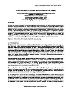
more central than a vertex v if its radius maxw c({u, w}) < maxw c({v, w}). Unfortunately, we have found that natural strategies for adjusting degree allocations lead to only marginal improvement in the diameters of the resulting trees. It appears difficult to find good degree allocations, independently of the tree building process. We have found that a more productive approach is to use a “loose degree allocation” and allow the tree-building process to construct a suitable tree satisfying the degree limits imposed by the loose allocation. Loose degree allocations are derived from the most balanced allocation by allowing small increases in the degrees of vertices. By combining the tree building procedure, with a specific rule for selecting eligible pairs and a procedure for “loosening” a degree allocation, we can define iterative algorithms for the overlay multicast routing problem. We start with a balanced degree allocation and build a tree using that allocation. If the resulting tree satisfies the diameter bound, we stop. Otherwise we loosen the degree allocation and build a new tree. We continue this process until we find a tree with small enough diameter, or until a decision is made to terminate the process and give up. The degree loosening procedure increases by 1, the degree allocation of up to b vertices, where b is a parameter. The first application of the procedure adds 1 to the degree allocation of the b most central vertices. If incrementing the degree allocation for a vertex v would cause its degree allocation to exceed the degree bound for v, then v’s degree allocation is left unchanged. The second round of the procedure adds 1 to the next b most central vertices (again, so long as this would not cause their degree bounds to be exceeded). Subsequent applications affect the degree bounds of successive groups of b vertices, and the process wraps around to the most central vertices, after all vertices have been considered. The process can be stopped after some specified number of applications of the degree loosening procedure, or after all degree allocations have been increased to the smaller of their degree bounds and k − 1 where k is the session fanout. If we select eligible pairs for which the connecting edge has minimum cost, the resulting algorithm is called Iterative Closest Pair (ICP) algorithm. If we select eligible pairs so as to minimize the diameter of the resulting component, the algorithm is called Iterative Compact Component (ICC) algorithm. In the Iterative Compact Tree (ICT) algorithm, we select eligible pairs, with one vertex of each pair in a single tree being constructed, and the other selected to minimize the tree diameter. This procedure is repeated for all possible initial vertices. An example execution of the ICT algorithm appears in Figure 3. For simplicity, we used geographical distance as routing cost and a diameter bound of 8000 km. Initially, the BDA output dictates the creation of a star topology with New York City as the center with degree of 7; this exceeds the diameter bound. In the second round, the degree allocation of the three nodes with small radius, Las Vegas, Phoenix, Louisville, is loosened by 1; this results in a smaller diameter tree satisfying the diameter bound. We observe that the actual degree allocation is still close to the balanced degree allocation. IV. BANDWIDTH D IMENSIONING The objective of the bandwidth dimensioning process is to assign access bandwidth to individual MSNs so as to maximize the number of sessions that can be served. The process allocates bandwidth subject to a bound on the total
10
Portland (1)
New York City (7)
Portland (1)
New York City (7)
Washington D. C. (1) Las Vegas (1)
Washington D. C. (1) Las Vegas (2)
Louisville (1)
Louisville (2) Phoenix (2)
Phoenix (1)
St. Petersburg (1)
Miami (1)
St. Petersburg (1)
Miami (1)
(a) Longest Path: Portland → New York → Phoenix;
(b) Longest Path: Portland → Las Vegas → Phoenix →
Length = 9416.67 km
Louisville → New York → St. Petersburg; Length = 7823.64 km
Fig. 3. An Example of the ICT Algorithm with Degree Adjustment
access bandwidth, reflecting practical cost constraints. The process involves one, or a series of traffic simulations, that provide information used to guide the allocation process. A. Baseline Dimensioning Our strategy for dimensioning the access bandwidth involves running traffic simulations, in which multicast sessions are created, routed and destroyed. The results of such simulations allow us to determine which MSNs are most limited by their access bandwidth and which have bandwidth to spare. This can be used to determine a better allocation, which can be used in subsequent simulations. However, since our routing algorithms use degree constraints implied by the bandwidth allocation to drive their route selections, we need an initial allocation in order initiate this iterative process. The approach we take is to perform a baseline simulation in which multicast routes are chosen with the objective of minimizing the diameter, without regard to degree constraints. In this simulation, a multicast session is rejected only if accepting it would cause the total access bandwidth in use to exceed the bound on the total access bandwidth. There are several ways to perform the route setup in the baseline simulation. The simplest is to select the minimum diameter spanning tree for a fanout n multicast session. As the baseline simulation is carried out, the average access bandwidth used at each MSN is recorded. In the resulting allocation, bandwidth is divided among MSNs in proportion to their average bandwidth use in the dimensioning process. Figure 4 shows an example result of this dimensioning process. For this example, MSNs were placed in each of the 50 largest metropolitan areas in US [25] and the geographic distances between cities was used as the link cost. The session arrival process is Poisson and the holding time follows a Pareto distribution. The session fanout follows a truncated binomial distribution with a mean of 10 and a minimum of 2. The distribution is obtained by shifting the binomial distribution on the interval [0, 48] to the interval of [2, 50]. The probability that a given MSN participates in a particular multicast session is proportional to the population of the metropolitan area that it serves. Each branch of a multicast session is assumed to require one unit of bandwidth and the total access bandwidth is 10,000 units, leading to an average allocation per MSN of 200.
0
0
20
30
Buffalo Hartford Providence Austin
Nashville
Memphis Rochester Raleigh Jacksonville Oklahoma City Grand Rapids West Palm Beach Louisville Richmond
St. Louis
10
Denver Pittsburgh St. Petersburg Portland Cincinnati Kansas City Sacramento Milwaukee Virginia Beach San Antonio Indianapolis Orlando Columbus Charlotte Las Vegas New Orleans Salt Lake City
Miami Seattle
200
Phoenix Cleveland Minneapolis San Diego
Houston Atlanta
New York Los Angeles
400
Boston
Bandwidth Units
600
Washington D.C. San Francisco Philadelphia Detroit
800
Dallas
Chicago
11
40
50
Fig. 4. Dimension of Server Access Bandwidth
The bandwidth allocation is driven by two factors: the number of sessions different MSNs participate in and their locations. Centrally located MSNs serve as natural branch points for multicast sessions and so get larger allocations than cities of comparable size that are further from the center of the country. This effect is apparent in Figure 4. In the figure, the cities are ordered by population on the x-axis, making the effects of location on the bandwidth allocation apparent in the “spikes” in the distribution. For example, the Chicago area has about 43% of New York’s population but receives 1.3 times more bandwidth. B. Iterative Dimensioning Given a baseline allocation, we can perform another traffic simulation using a specific routing algorithm of interest. The results from this simulation can be used to determine a new allocation, which we expect to be a better match for our routing algorithm. By iterating this process, we can refine the allocation further. To make this precise, let C i be the capacity assigned to MSNi in one step of the dimensioning process. We reallocate access bandwidth by letting the new bandwidth Ci0 = Li + (1/n)
P
Ri , where n is the number of MSNs, Li is the average access bandwidth usage of MSNi
during the simulation and Ri = Ci − Li is the average unused bandwidth of MSNi . Intuitively, the algorithm converges since the routing algorithm tries to equalize the residual degrees by configuring multicast sessions to branch at nodes with the most unused capacity. The dimensioning process also reduces the excess capacities of big nodes and add them to those whose bandwidth are less abundant. In reference [24], we showed that by tightly coupling the dimensioning process to the routing algorithm, we improve on the overall network utilization. V. E VALUATION
OF
ROUTING A LGORITHMS
This section reports simulation results for the overlay multicast routing algorithms described above. We report results for three network topologies and a range of multicast session sizes. The principal performance metric is the multicast session rejection rate.
12
Seattle Portland
Sacramento
Minneapolis
Denver Las Vegas
Los Angeles
Phoenix
San Diego
Buffalo Cleveland
Chicago
Salt Lake City
San Francisco
Rochester Detroit
Boston Providence New York City
Cincinnati Virginia Beach St. Louis Kansas City Raleigh Charlotte Nashville Oklahoma City Memphis Atlanta Dallas Jacksonville Austin Orlando San Antonio New Orleans Houston
St. Petersburg
(a) 50 Largest U.S. Metropolitan Areas
Miami West Palm Beach
(b) Disk Configuration
(c) Sphere Configuration
Fig. 5. Overlay Network Configurations
A. Simulation Setup We have selected three overlay network configurations for evaluation purposes. The first (called the metro configuration) has an MSN at each of the 50 largest metropolitan areas in the United States [25]. The “traffic density” at each node is proportional to the population of the metropolitan area it serves. We use a Poisson session arrival process and the session holding times follow a Pareto distribution. Session fanout follows a truncated binomial distribution with a minimum of 2 and maximum of 50, and means varied in different result sets. In the rest of the paper, when we refer to a session fanout as k, then k is the mean fanout of the binomial distribution. All multicast sessions are assumed to have the same bandwidth. Different MSNs were assigned different interface bandwidths, depending on their traffic density and their location. MSNs in more central locations are assigned higher interface bandwidths than those in less central locations, since it is more efficient for multicast sessions to branch out from these locations than from the more peripheral locations. The assignment of interface bandwidth at MSNs is critical to the performance of the routing algorithms. We have dimensioned the network to best carry a projected traffic load given a specific routing algorithm as described in the previous section. The metro configuration was chosen to be representative of a realistic overlay multicast network. However, like any realistic networks, it is somewhat idiosyncratic, since it reflects the locations of population centers and the differing amounts of traffic they produce. The other two configurations were chosen to be more neutral. The first of these consists of 100 randomly distributed nodes on a disk and the second consists of 100 randomly distributed nodes on the surface of a sphere. In both cases, all nodes are assumed to have equal traffic densities. In the disk, as in the metro configuration, the MSN interface bandwidths must be dimensioned, but in this case it is just a node’s location that determines its interface bandwidth. In the sphere configuration, all nodes are assigned the same interface bandwidth, since there is no node that is more central than any other. The three network configurations are illustrated in Figure 5. In all configurations, the geographical distance between two nodes is taken as the cost of including an edge between those nodes in the multicast session tree.
13
B. Comparison of Tree Building Techniques In the previous section, we suggested three basic tree building techniques: selecting the closest pair (CP), selecting the pair that minimizes the component diameter (CC), and selecting the pair that minimizes the single tree diameter (CT). The iterative versions of these algorithms, namely ICP, ICC and ICT, seek to satisfy the diameter bound by loosening the degree allocation produced by BDA. In this section, we examine their performance sensitivities to different diameter bounds and to the number of rounds allowed for degree adjustment. The simulation uses the metro configuration as the network topology and a mean session fanout of 10. Figure 6 shows the session rejection rates versus the ratio of the diameter bound to the maximum inter-city delay (6000 km). In this simulation, we allow each algorithm to loosen the degree allocation as many rounds as possible, until it reaches the smaller of nodes’ degree bounds or k − 1, where k is the session size. The horizontal line labeled as BDA, shows the rejection rate using the balanced degree allocation strategy, but ignoring the diameter of the resulting tree. Offered Load = 0.75
0
10
ICP ICC BCT ICT
−1
Rejection Rate
10
−2
10
−3
10
−4
10
Offered Load = 0.75
0
10
−1
10
−2
10
−3
10
−4
ICT ICC ICP
BDA
−5
10
Rejection Rate
10
1
1.2 1.4 1.6 1.8 2 Diameter Bound / Maximum Inter−city Distance
Fig. 6. Sensitivity to Diameter Bound
0
2 4 6 8 Maximum Degree Adjustment Round
10
Fig. 7. Sensitivity to Degree Adjustment Round
As the large cities in this map are along the coastal areas, the majority of the sessions will span across the continent. Therefore, it is difficult to find a multicast tree for these sessions when the diameter bound is tight, resulting in very high rejection rates for all algorithms. However, as the diameter bound is relaxed, the rejection rate improves for all the algorithms, with the iterative algorithms all achieving essentially the same performance for diameter bounds of more than 1.8 times the maximum inter-city distance. At intermediate diameter bounds, the ICT and BCT algorithm performs better than the ICC and ICP algorithms. This suggests that building from a single tree, as both ICT and BCT do, is more effective in minimizing the tree diameter. The BCT algorithm does not allocate its node degree before building the tree; rather, it seeks to maximize the residual bandwidth as the algorithm progress. For large diameter bounds, BCT is not able to reduce its rejection rate as much as the algorithms using balanced degree allocation. Figure 7 shows the rejection ratio versus the maximum number of degree adjustment rounds allowed in ICP, ICC and ICT. The diameter bound is fixed at 8000 km for this simulation. In each degree adjustment round, the number of
14
vertices being adjusted is 3. Generally, the ICP and ICC algorithms only benefit from the very first few rounds of degree adjustment, which allows nearby nodes to be joined together to form collections of small forests. The additional rounds of degree adjustment have no effect on them and the rejection rates remain relatively high. Contrarily, the ICT algorithm benefits greatly from the additional rounds of degree adjustment. It is able to utilize the increased degree allocation at the centrally located nodes and form smaller diameter trees. We conclude in this subsection that the ICT algorithm, when combined with the degree loosening procedure, is more effective at producing small diameter trees than ICP and ICC. In the rest of this paper, we will focus our evaluation mainly on the ICT algorithm. However, ICT’s greater effectiveness comes with a cost of added complexity, as it iterates through each possible starting vertex in order to find the best tree. We will analyze the computational cost of the ICT algorithm later in the section. C. Performance Results – Rejection Rate Figure 8 shows the session rejection rates versus offered load for a subset of the overlay multicast routing algorithms presented earlier. The charts also include a lower bound on the rejection fraction that was obtained by running a simulation in which a session is rejected only if the sum of the degree bounds at all nodes in the network is less than 2(k −1) where k is the number of nodes in the session being set up. The lower bound curves are labeled LB. The results, labeled BDA, are obtained using the balanced degree allocation strategy, and ignoring the diameter of the resulting tree. We conjecture that this also represents a lower bound on the best possible rejection fraction that can be obtained by any on-line routing algorithm. It is certainly a lower bound for algorithms based on the balanced degree allocation strategy. For these charts, the diameter bound for the metro configuration is 8000 km which is approximately 1.5 times the maximum distance between nodes. For the disk and sphere topology, the bound is two times the disk diameter and three times the sphere diameter; each is about twice the maximum distance between any two nodes. The total interface bandwidth for all MSNs is 10,000 times the bandwidth consumed by a single edge of a multicast session tree. So, in the sphere, each MSN can support a total of 100 multicast session edges and for the metro configuration, the average number is 200. Reference [24] shows the performance sensitivity to the total available interface bandwidth: the larger the capacity, the lower the rejection rate. Overall, the results show that the algorithms that seek to balance the residual degree usually perform much better than the CT algorithm, which merely seeks to minimize the diameter subject to a constraint on the maximum degree bound of a node (dmax (v)). The performance of CT is particularly poor in the fanout 20 case, since it tends to create nodes with large fanout leading to highly unbalanced residual degree distributions. Looking down each column, we see that the lower bound increases with the fanout. This simply reflects the fact that each session consumes a larger fraction of the total interface bandwidth. For the sphere, the rejection fraction also increases with fanout for the BDA curve. This makes sense intuitively, since as the fanout grows, one expects it to be more difficult to find balanced trees with small enough diameter. In the disk and metro configurations, it is less clear
15 disk, fanout = 5
US Metro Map, fanout = 5
0
LB BDA ICT BCT CT
0
LB BDA ICT BCT CT
10
−2
10
10
−2
10
−3
10
LB BDA ICT BCT CT
−1
Rejection Rate
10
10
−1
Rejection Rate
−1
Rejection Rate
sphere, fanout = 5
0
10
10
−2
10
−3
−3
10
10
−4
10
−4
0.5
0.6
0.7
0.8
0.9
1
10
1.1
−4
0.5
0.6
0.7
Offered Load
10
1.1
LB BDA ICT BCT CT
0.6
LB BDA ICT BCT CT
−1
Rejection Rate
−2
0.8 0.9 Offered Load
1
1.1
0
10
10
0.7
10
LB BDA ICT BCT CT
−1
10 Rejection Rate
−1
10
0.5
sphere, fanout = 10
0
10
10
Rejection Rate
1
disk, fanout = 10
US Metro Map, fanout = 10
0
0.8 0.9 Offered Load
−2
10
−2
10
−3
10
−3
−3
10
10
−4
10
0.5
0.6
0.7
0.8
0.9
1
−4
10
1.1
−4
0.5
0.6
0.7
Offered Load
10
−1
LB BDA ICT BCT CT
−2
10
LB BDA ICT BCT CT
−3
0.7
0.8 Offered Load
0.9
1
1.1
10
1.1
−2
10
LB BDA ICT BCT CT
−3
10
−4
0.6
1
−1
10
−4
0.8 0.9 Offered Load
10 Rejection Rate
Rejection Rate
−2
10
0.5
0.7
0
−1
−3
0.6
10
10
10
0.5
sphere, fanout = 20
0
10 Rejection Rate
1.1
10
10
10
1
disk, fanout = 20
US Metro Map, fanout = 20
0
0.8 0.9 Offered Load
−4
0.5
0.6
0.7
0.8 0.9 Offered Load
1
1.1
10
0.5
0.6
0.7
0.8 0.9 Offered Load
1
1.1
Fig. 8. Rejection Fraction Comparison
why the BDA curve changes with fanout as it does. Part of the explanation for the observed behavior is that the network dimensioning process is based on an assumed traffic load, and in particular, an assumed multicast session fanout of 10. When the simulated traffic has the same fanout distribution as the one used to dimension the network, we get smaller rejection rates. However, there is a somewhat surprising deterioration of the rejection rate for small fanout, particularly in the metro network case. The apparent explanation for this is that with small fanout, we often get sessions involving MSNs near the east and west coasts, but none in the center of the country. Such sessions are unable to exploit the ample unused bandwidth designed into the more central MSNs, based on a larger average fanout. A similar effect is observed with the disk, but it is more extreme in the metro configuration because of the greater population densities on the coasts, and also the smaller ratio of the diameter bound to the maximum inter-MSN distance (1.5 vs. 2). The curves for the ICT algorithm are generally quite close to the BDA curves, leaving little apparent room for
16
improvement. There are small but noticeable gaps in a few cases. For the metro configuration, the gaps for fanout 5 and 20 are most probably due to the difference between the average fanout of the simulated traffic and the fanout used for dimensioning. This explanation does not account for the gap in the sphere configuration for fanout 20, since in the sphere, all nodes have the same interface bandwidth. The most plausible explanation seems to be that with large fanout, it just becomes intrinsically more difficult to find trees that satisfy the diameter bound. In three out of the nine cases shown, the BCT algorithm performs nearly as well as the ICT algorithm. Its performance relative to ICT is worst for the sphere and best for the metro configuration. D. Performance Results – Tree Diameter Next, we investigate the performance of these algorithms in terms of the tree diameter they created. Figure 9 shows the cumulative distribution of the tree diameter scaled to the diameter bound used in the algorithms. The fanout used here is 10 per session. Also, we show in a table the mean and variance of the tree diameter using unscaled value. Disk
US Metro Map
1 ICT BCT CT
0.8 0.6 0.4 0.2
0
0.2 0.4 0.6 0.8 Diameter / Bound (8000km)
ICT BCT CT
0.8 0.6 0.4 0.2 0
1
1
Cumulative Percentage
Cumulative Percentage
Cumulative Percentage
1
0
Sphere
0.6 0.4 0.2 0
0
0.2
0.4
0.6
0.8
ICT BCT CT
0.8
1
0
Diameter / Bound (2*D)
metro
disk
0.2 0.4 0.6 0.8 Diameter / Bound (3*D)
1
sphere
mean
std.
mean
std.
mean
std.
CT
5581.22
14.4%
222.38
13.9%
429.16
10.0%
BCT
5627.77
14.5%
222.67
14.5%
428.17
10.1%
ICT
6347.36
15.7%
248.17
19.9%
516.18
10.4%
Fig. 9. End-to-end Delay performance
We observe that the diameter performance of the BCT algorithm is as good as that of the CT algorithm; the difference is almost indiscernible. The ICT algorithm does, however, show a performance degradation on the tree diameter. Especially in the sphere, ICT generates trees with diameter much larger than those generated by the other two algorithms. This is due to that traffic load tends to be more evenly distributed in the sphere configuration and BDA is very effective at equalizing the available capacity at each MSN, that it tends to produce degree allocations with large numbers of vertices of degree 2, resulting in long paths. The different performance characteristics of the ICT and BCT algorithms suggests that it may make sense to use BCT for application sessions that require better end-to-end delay performance, and use ICT algorithm for others. Although
17
we have not investigated the system utilization when both algorithms are used, we conjecture that it should probably do better than the BCT algorithm. E. Complexity of the ICT Algorithm Although the ICT algorithms gives superior performance on the overall system utilization and can satisfy the diameter bound in most cases, it potentially has the disadvantage of higher computational complexity. Especially with a more stringent diameter bound, as the algorithm continues to loosen the nodes’ degree allocation in a round by round basis in order to search for an appropriate tree, the complexity goes higher as well as the rejection ratio. Computation Complexity fanout = 10, offered load = 0.75
0.2
0.1
0
5 4 3 2 1
1.5
1.6
1.7 1.8 1.9 Diameter bound / Disk diameter
2
0
Average round of relaxation
Fraction of sessions for relaxation
0.3
Fig. 10. Computation Complexity of the ICT Algorithm
In Figure 10, we plotted the computation requirement for the ICT algorithm on a disk topology with session fanout equal to 10. The top half of the figure shows the percentage of sessions that require degree adjustment; and the bottom half shows the average number of rounds iterated for these sessions. We observe that the actual number of additional rounds is reasonably low. For instance, if the diameter bound is 1.7 times the disk diameter, 10% of the sessions require an average of 2 rounds of degree adjustment. However, if the diameter bound is too stringent, the extra rounds of degree adjustment do not help much in reducing the session rejection rate (not shown). Therefore, it is important to pick a suitable diameter bound for a topology so that the algorithm can operate more efficiently and more effectively. From our experience, a bound of twice the maximum distance between any pair of nodes seem to be a good choice in all three network configurations. VI. A H YBRID S CHEME
OF
CP
AND
CT A LGORITHMS
We observe from the previous section the two different aspects of the ICP and the ICT algorithms. The ICP algorithm has the complexity of O(n2 log n), much less than the ICT algorithm which is O(n3 ) for each initial vertex. Though simpler, ICP is not very effective in finding smaller diameter trees, leading to high session rejection rate even at light traffic load. On the other hand, the complexity of the ICT algorithm is exacerbated in sessions with larger fanout. In order to improve its efficiency, we investigate a hybrid scheme of ICP and ICT.
18
The hybrid scheme starts the same as CP, joining closest eligible pairs into components with respect to the output of the BDA strategy. When there are k components left, the hybrid scheme switch to the CT algorithm, joining the components by minimizing the multicast tree diameter. The complexity of joining k components using the CT algorithm, is O(k 2 n2 ), including the iteration of each component as the initial component. As before, the process is repeated with rounds of degree loosening, until we find a multicast tree that satisfies the diameter constraint.
−1
10
−2
10
−3
10
−4
sphere, fanout = 20
0
0
10 BDA ICT hybrid, g = 4 hybrid, g = 6 hybrid, g = 10
10 BDA ICT hybrid, g = 4 hybrid, g = 6 hybrid, g = 10
−1
10
−1
10 Rejection Rate
10
disk, fanout = 20
US Metro Map, fanout = 20
0
Rejection Rate
Rejection Rate
10
−2
10
−3
10
−4
0.6
0.7
0.8 Offered Load
0.9
1
1.1
10
BDA ICT hybrid, g = 4 hybrid, g = 6 hybrid, g = 10
−3
10
0.5
−2
10
−4
0.5
0.6
0.7
0.8 0.9 Offered Load
1
1.1
10
0.5
0.6
0.7
0.8 0.9 Offered Load
1
1.1
Fig. 11. Performance of the hybrid CP and CT Algorithms
Figure 11 shows the performance of the hybrid scheme on three network topologies, with session size equal to 20. When k is small, the hybrid scheme inherits the same problem as the ICP algorithm, and is ineffective to satisfy the diameter constraint. This is especially true for the sphere configuration, where ICP results in long legged paths in the tree. However, by increasing k, the hybrid scheme gains quickly in its ability in finding a smaller diameter tree and brings down the total rejection rate. The hybrid scheme shows better performance on the disk configuration. This suggests that it is more useful to reduce the computational complexity when the diameter constraint is less stringent. VII. R ELATED W ORK The Multicast Backbone (Mbone) [7], is the best known and widely adopted multicast overlay network. The Mbone is implemented as tunnels at the network layer and implements distance vector multicast routing protocol [2]. Other standard routing protocols include: core-based tree (CBT) [3], protocol independent multicast (PIM) [8] and most recently, source specific multicast (SSM) [15]. All of these routing protocols build shortest path trees from data sources or from the core node of a session, to minimize network delay. There are a number of application-level multicast services appearing in the recent literature, mostly due to the dwindling usage on the Mbone and the slow deployment of network multicast services. The flexibility of application-level multicast services allows the routing policy to be changed based on the target application requirements. For example, Scattercast [5] uses delay as the routing cost and builds shortest path trees from data sources; Overcast [18] explicitly measures available bandwidth on an end-to-end path and builds a multicast tree by maximizing the available bandwidth from the source to the receivers; and Endsystem multicast [16] uses a combination of delay and available bandwidth, and prioritizes available bandwidth over delay when selecting a routing path.
19
In this paper, we have defined interface bandwidth as our primary routing metric. The path selection policies seek to optimize the usage of interface bandwidth of MSNs while satisfying the end-to-end delay performance of individual sessions. As a result, our routing algorithms differ fundamentally from all of the above. The pioneering work on network design can be traced back to the early 60s and 70s by Kleinrock [19] and Schwartz [22], among several others. They investigated a much broader design problem relating to the topological design, capacity allocation, routing and flow control aspects of computer networks in a point-to-point communication environment. In their network model, a traffic matrix is known in advance and the cost of the network relates to the number of network links and link capacities. The goal is to find the least cost network that minimizes the average message delay time or limits the maximum message delay time between any pair of nodes. By applying queuing theory, they allocate the optimal capacity to each link and compute the total network cost. The least cost network among a set of varied network topology is then chosen. The fundamental difficulty in applying a similar principle to overlay multicast network design, is the complexity involved in computing the related parameters in a multicast fashion. Particularly, there are n n−2 ways of establishing a multicast tree for an session size of n, making it impossible to compute the traffic statistics on any of the paths. Moreover, the multicast traffic also depends on parameters such as the size of the sessions, the set of nodes involved in each session, etc, which are not present in a unicast environment. These added complexities ultimately result in our simulation-based approach to solve the combined dimensioning and multicast routing problem. VIII. C ONCLUSIONS In this paper, we have introduced several multicast routing algorithms that are specifically designed for overlay networks, where the optimization of the interface bandwidth at multicast service nodes is a primary focus. This leads to rather different routing considerations than in conventional networks. Our algorithms seek to balance the available MSN interface bandwidth while keeping the tree diameter small. Our evaluation showed that it is possible to achieve a large gain in system utilization without a significant reduction in the end-to-end delay performance. The algorithms perform well across a range of network configurations and traffic conditions. Perhaps the most promising direction for future work on overlay multicast routing relates to the dynamic version of the problem. Another direction worth pursuing is the development of routing algorithms that provide fault tolerance in the presence of server failures. R EFERENCES [1]
Akamai Technologies, Inc. http://www.akamai.com.
[2]
F. Baker. Distance Vector Multicast Routing Protocol - DVMRP. RFC 1812, June 1995.
[3]
A. Ballardie. Core Based Trees (CBT version 2) Multicast Routing - Protocol Specification. RFC 2189, September 1997.
[4]
A. Cayley. On the Theory of Analytical Forms Called Trees. Philosophy Magazine, 13, 1857.
[5]
Y. Chawathe, S. McCanne, and E. Brewer. An Architecture for Internet Content Distribution as an Infrastructure Service. Unpublished, available at http://www.cs.berkeley.edu/ yatin/papers.
[6]
T. H. Cormen, C. E. Leiserson, and R. L. Rivest. Introduction to Algorithms. MIT Press, 1990.
20
[7]
H. Erikson. MBONE: The Multicast Backbone. Communication of the ACM, pages 54–60, August 1994.
[8]
D. Estrin, V. Jacobson, D. Farinacci, L. Wei, S. Deering, M. Handley, D. Thaler, C. Liu, S. P., and A. Helmy. Protocol Independent Multicast-Sparse Mode (PIM-SM): Motivation and Architecture. Internet Engineering Task Force, August 1998.
[9]
P. Francis. Yallcast: Extending the Internet Multicast Architecture. http://www.yallcast.com, September 1999.
[10] M. R. Garey and D. S. Johnson. Computers and Intractability : A Guide to the Theory of NP-Completeness. San Francisco : W. H. Freeman, 1979. [11] S. Hakimi. Optimal Locations of Switching Centers and Medians of A Graph. Operations Research, 12:450–459, 1964. [12] R. Hassin and A. Tamir. On the Minimum Diameter Spanning Tree Problem. Information Processing Letters, 53(2):109–111, 1995. [13] J. Ho, D. Lee, C. Chang, and C. Wong. Minimum Diameter Spanning Trees and Related Problems. SIAM J.Comput., 20(5):987–997, 1991. [14] D. Hochbaum. Approximation Algorihtms for NP-Hard Problems. Brooks/Cole Publishing Co., 1996. [15] H. Holbrook and B. Cain. Source Specific Multicast. IETF draft, draft-holbrook-ssm-00.txt, March 2000. [16] Y. hua Chu, S. G. Rao, S. Seshan, and H. Zhang. Enabling Conferencing Applications on the Internet Using an Overlay Multicast Architecture. In Proc. ACM SIGCOMM 2001, San Diago, CA, August 2001. [17] iBeam Broadcasting Corp. http://www.ibeam.com. [18] J. Jannotti, D. K. Gifford, K. L. Johnson, M. F. Kaashoek, and J. W. O. Jr. Overcast: Reliable Multicasting with an Overlay Network. In Proc. OSDI’01, 2000. [19] L. Kleinrock. Communication Nets: Stochastic Message Flow and Delay. McGraw-Hill, New York, 1964. [20] D. Pendarakis, S. Shi, D. Verma, and M. Waldvogel. ALMI: An Application Level Multicast Infrastructure. In 3rd USENIX Symposium on Internet Technologies and Systems (USITS’01), San Francisco, CA, March 2001. [21] R. Ravi, M. Marathe, S. Ravi, D. Rosenkrantz, and H. H. III. Many birds with one stone: Multi-objective approximation algorithms. In Proc. of the 25th ACM Symposium on Theory of Computing, 1993. [22] M. Schwartz. Computer-Communication Network Design and Analysis. Prentice Hall, 1977. [23] S. Shi. Design of an Internet Multicast Architecture Using Overlay Networks. PhD thesis, In Preparation, Department of Computer Science, Washington University, 2002. [24] S. Shi, J. Turner, and M. Waldvogel. Dimension Server Access Bandwidth and Multicast Routing in Overlay Networks. In 11th International Workshop on Network and Operating System Support for Digital Audio and Video (NOSSDAV’01), June 2001. [25] U.S. Census Bureau. http://www.census.gov/population/www/estimates/metropop.html. [26] S. Zhuang, B. Zhao, A. D. Joseph, R. H. Katz, and J. Kubiatowicz. Bayeux: An Architecture for Wide-Area, Fault-Tolerant Data Dissemination. In Proc. NOSSDAV’01, June 2001.