Multipath Routing in Wireless Mesh Networks ∗
Marc Mosko∗
Palo Alto Research Center 3333 Coyote Hill Road Palo Alto, CA 94304 Email:
[email protected]
Abstract— This paper addresses multipath routing in a mobile wireless network. We review the premise that a routing protocol should prefer disjoint path construction and argue that using disjoint paths limits route reliability in mobile ad hoc networks compared to using multiple loop-free paths that need not be disjoint. In a mobile ad hoc network, link lifetimes may be relatively short compared to traffic flows. The characteristics of a MANET are significantly different than the networks considered by Kleinrock in his original delay analysis of alternate path routing. In particular, on-demand routing protocols may suffer a significant delay during path discovery. We argue that a routing protocol should exploit the mesh connectivity over non-disjoint loop-free paths to improve s, t-connectedness lifetime in a mobile network. Exploiting mesh connectivity amortizes expensive path discovery operations and may lead to better performance than using disjoint or maximally disjoint paths.
I. I NTRODUCTION The main objective of using multipath routing in a mobile ad hoc network is to use several good paths to reach destinations, not just the one best path [1], without imposing excessive control overhead in maintaining such paths. Multipath routing has long been recognized as an important feature in networks to adapt to load and increase reliability [2], [3]. Telecommunication networks adopted alternate path routing, really a form of path failover, in 1984 [4]. Many routing papers on ad hoc routing suggest that the proposed routing protocol may operate correctly (i.e., provide multiple loopfree paths), without specifically addressing the performance of the protocol when multipaths1 are used [5]–[9]. Other protocols suggest building alternate paths, but without claims of correct operation (e.g. [10]–[13]). Several papers measure route coupling [14]–[16], the mutual interference of routes in a common-channel multi-hop ad hoc network, and find routes with low coupling. Route coupling, however, makes every flow dependent on every other flow through an area and the papers on route coupling do not address the cost of maintaining lowcoupled routes in an on-demand protocol; they typically use link-state pro-active protocols. Most of the works on ad hoc multipath restrict the number of potential routes to a small number, usually two. AOMDV [17] allows up to k link-disjoint RREPs, where one is the “quickest” path and the others are chosen from the next link-disjoint RREQs. SMR [18] builds two paths from the quickest RREQ and then collects RREQs 1 We use the term ”multipath” to denote a set of multiple paths to a destination that need not be node or edge disjoint.
†
J.J. Garcia-Luna-Aceves∗†
Computer Engineering Department University of California at Santa Cruz Santa Cruz, CA 95064 Email:
[email protected]
for a period and chooses a second maximally disjoint path from the first. In a zone-disjoint scheme [16], only two paths are built, but they are not necessarily minimum. This scheme uses an iterative algorithm to discard the worst choice each round until only two paths are left. In this paper, we argue that a routing protocol for ad hoc networks should fully exploit the rich connectivity of the network to improve the reliability of packet delivery. In a nutshell, a well-designed multipath routing protocol should find many alternate loop-free paths to destinations and should keep those paths alive by sending some amount of data traffic over them as a function of their quality. Paths with poor quality or significantly longer distance should not be used. The exact methods used by a routing protocol to propagate metrics and distribute load between paths is an open question. Interestingly, a number of routing protocols for ad hoc networks that attempt to take advantage of multiple paths to destinations advocate the use of node- or edge-disjoint paths. Section II surveys the literature and makes the case that disjoint paths are not necessary to improve the reliability of wireless ad hoc networks. Furthermore, Section III shows that multiple well-connected loop-free paths offer substantially longer path lifetimes than sets of disjoint paths. Based on these results, Section IV illustrates a multipath routing approach in which node or edge disjoint paths are not enforced, using the DOS [19] routing protocol as an example. Section V summarizes the implementation of DOS used in the simulation study presented in Section VI, which compares the path distributions of our loop-free on-demand routing protocol and shows that we can maintain between 1.2 and 1.5 paths per hop, without any special path maintenance mechanisms. In 100-node simulations, the multipath scheme has about 1/3 the network load of min-hop multipath and a slightly higher delivery ratio. II. P RIOR W ORK In the literature, there are several types of disjoint paths. In two node disjoint paths, P1 and P2 , there is no common nodes except the first (source) and last (destination). In link disjoint paths, there are no common edges, though there may be common nodes. P1 = {s, a, b, c, t} and P2 = {s, m, b, n, t} are two link-disjoint paths, although they share the node b. There are also zone disjoint paths, which try to keep paths separated by some number of hops. Two “maximally”
disjoint paths mean that among some set of choices P1...k , the maximally disjoint paths share the fewest nodes or edges in common. There is little difference between link-disjoint and node-disjoint schemes. In the literature, it is often assumed that nodes are fail-safe and only links fail. If nodes have a failure probability, a node-splitting scheme may be employed to split a failure-prone node in to two fail-safe nodes and join them by a link with the equivalent failure probability [20]. Wireless ad hoc networks embody a different routing and delay paradyne than traditional wired networks. In wired networks, paths are generally long lived with respect to traffic flows, network control overhead is usually very small compared to data, and path discovery time short due to proactive protocols (e.g. OSPF [21]). Wireless ad hoc networks are significantly different. Due to mobility and interference, particular edges have a short life compared to traffic flows. This may be exacerbated if a routing protocol breaks paths too aggressively due to packet loss. Network control overhead may be very high: more than one control packet per data packet delivered. Path discovery times in on-demand protocols may be significant, depending on packet loss and network congestion if for no other reason than contention-based MAC protocols may have very long channel access waiting times. Important early work on the allocation of flows to a network make certain assumptions that are not necessarily true any more in mobile ad hoc networks. Kleinrock’s early work on network message delay [3, p. 21] defines a “fixed routing procedure” as a single-path route plan given the source and destination of a message. An “alternate routing procedure” allows multiple paths. Kleinrock shows that under optimal capacity assignment to a given graph with independent links, messages experience shorter delays with fixed routing than using an alternate routing approach. Kleinrock, however, qualifies the delay benefits of fixed routing by noting that if there is not an optimal capacity assignment or if the topology changes in such a way that alternate path routing can adjust traffic flows, then alternate routing may be superior in terms of delay [3, p. 27]. Kleinrock finds that a simple proportional routing scheme, where links receive a share of the traffic proportional to their capacity, may be a satisfactory alternate routing scheme so long as one is careful about high load situations. Cantor and Gerla’s paper on optimal (minimum delay) routing [22] and Gallager’s paper on minimum delay routing [23] adopt Kleinrock’s formulation of delay, but neither restrict the traffic flow k to disjoint paths. The routing assignment variable αij (Cantor and Gerla) or φik (j) (Gallager) allow dynamic proportional routing over many multipaths. Suurballe [24] motivates his work on disjoint paths through the survivability of a network being related to the number of node disjoint paths. Similar to Baran’s early work [2], this notion of network design is based on the assumption of node destruction causing network partition. Node disjoint paths are preferable because new links cannot be setup quickly and there is an inherent static assumption (cities do not move). Ogier and Schacham’s work [25] on finding pairs of shortest disjoint paths is motivated by Chiou and Li’s work on two-
copy routing [26], which in turn basis the claim of disjoint paths on their earlier work [27]. The work of Chiou and Li [27] asserts that it is desirable for reliability to send packets along disjoint paths. This assertion is not specifically argued, but it is stated that in two-copy routing (where a single message is sent twice in the network) it is preferable to use two disjoint paths “in order to minimize the probability of losing both copies.” This, of course, clearly depends on the reliability of each path. Under the assumptions of the paper, each link has a successful operation probability pi that is independent of other links and instantaneous. This makes each hop a memoryless Bernoulli trial. So, given two disjoint paths P1 and P2 with equal reliability, it does not matter if you send the two copies over the same paths or over different paths. Each trial (copy) is independent. One would, of course, incur more delay sending two copies serially over one path rather than in parallel over two paths, all other things being equal. Chiou and Li [27] also assume a static routing protocol, which will not redirect traffic around faults. If failures are instantaneous, re-routing is not necessary assuming one is already using a good path. If failures, as they are in actual networks, persist for some time, re-routing is critical. They further discount “memoryless routing” (per-hop routing) because in an acyclic graph, there must be at least one node with a single route to the destination [27, lemma 1]. So this would argue for the use of a source-routing protocol. As is seen in the SMR protocol [18], the cost of maintaining two disjoint paths (SMR-1) in a source routing on-demand protocol is higher than building two paths, but waiting until they both fail (SMR-2). Nasipuri et al. [28], focus on the use of disjoint paths. Table 1 of their work compares a protocol where only the source maintains two disjoint paths (Protocol 1) and a protocol where the source and all intermediary nodes maintain disjoint paths (Protocol 2). They find in all the cases they examined, Protocol 2 has a lower rate of path discovery. In fact, the rate of path discovery decreases as the path length increases. It is interesting to note that, in effect, Protocol 2 assumes a “partial” mesh multipath. Clearly, the rate at which new paths need to be discovered after failures can be further reduced by allowing more redundancy among the loop-free paths between a source and a destination.
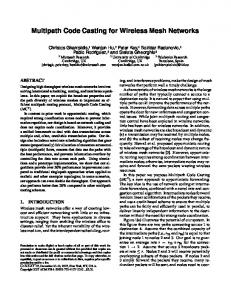
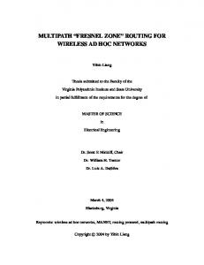
III. M ESH M ULTIPATH A NALYSIS To begin our discussion, let us consider the networks in Fig. 1. The top network shows disjoint s, t-connectivity and the bottom network shows a rich mesh connectivity. If we consider each link to have operational probability p, then it is a straightforward reliability calculation to determine the s, treliability of the networks. For our purposes, a minimal pathset (minpath) is the set of all loop-free paths between nodes s and t. Using the method of inclusion/exclusion on minpaths [29,
A
B
C
S
T D
E
F
A
B
C
S
T F
Fig. 1. 1
G
H
(a) disjoint paths (b) mesh multipath
Disjoint Mesh
Graph Reliability
0.8
0.6
0.4
0.2
0 0
0.2
Fig. 2.
0.4 0.6 Link operating probability
0.8
1
Network reliability
they formulate Protocol 2, let the primary path be k hops. Each node along the primary path has an alternate disjoint route to t, so there are k +1 minpaths. Protocol 1 only has two minpaths. This explains the phenomenon they observe that the rate of path discovery decreases as the path length increases. It is because with each extra hop along the primary path, they add another minpath. Let us consider the delay of an ad hoc network. One large delay component in an on-demand routing protocol is the process of path discovery. Typically, a node performs a type of expanding ring search. The NS2 v2.28 implementation of AODV [30], for instance, first tries a 5-hop search with 30ms per hop, so AODV would time out after 300ms before trying a 7-hop search which times out after 420ms, and then tries network-wide floods, each timing out after 1.8s. Because of the high cost of route discovery, we wish to amortize it over the lives of many paths. We can adapt the method of inclusion/exclusion reliability calculations to compute the distribution of time between path discoveries. Following [28], let each link have an independent mean lifetime of `, so λ = 1/`. The cumulative distribution function for link operation is F (t) = 1 − exp(−λt). For a series of k links, the CDF is Fs (t) = 1 − exp(−kλt). For a set of m parallel paths, each with a CDF of Fs (t), Fp (t) = (Fs (t))m . Using these results, the CDF for the disjoint network in Fig. 1 is Fdisj (t) = (1 − exp[−4λt])2 . (3) R∞ Using the relation that the expected value E[X] = 0 1 − F (x)dx [31, p. 93], the mean lifetime of the disjoint graph is Z ∞ Edisj [T ] = 2e−4λt − e−8λt dt 0
Sec 2.4.2], the reliability polynomials are: 4
8
Rel(disj) = 2p − p (1) 4 8 4 6 7 8 Rel(mesh) = 2p − p + (6p − 12p − 8p + 15p +12p9 − 20p10 + 8p11 − p12 ) (2) The disjoint network in Fig. 1(a) has two minpaths ({s, a, b, c, t} and reflection). The mesh network in Fig. 1(b) has eight minpaths ({s, a, b, c, t}, {s, a, b, h, t}, {s, a, g, h, t}, {s, a, g, c, t} and reflections). Fig. 2 plots the network reliability for the disjoint and mesh configurations. As one expects, the mesh configuration has a significantly higher reliability. In general, it is always the case that by adding an operational minpath to a graph, the graph reliability increases. In the formulation of reliability using Boolean algebras [29, Sec. 2.6], let P1 , . . . , Ph be the enumeration of minpaths and let the event Ei be the event that path Pi is operational. The Boolean formulation of reliability uses the events D1 = E1 E1 ∩ E2 ∩ · · · ∩ Ei−1 ∩ Ei . The reliability is and Di = P h Rel(G) = i=1 P rob[Di ]. Thus, adding a minpath never decreases the reliability. Of course, the marginal improvement in reliability could be very small. As noted above, Nasipuri et al. [28] actually uses a mesh multipath approach in the better-performing Protocol 2. As
=
3/(8λ)
(4)
This agrees with [28, Eq. 5]. To analyze the mesh graph, we use the inclusion/exclusion equation [29, p. 14] h X (−1)j+1 j=1
X
Prob[EI ]
(5)
I⊆{1,...,h},|I|=j
where EI is the event that all paths Pi with i ∈ I operate no longer than time t. Let n be the number of distinct links in EI , then Prob[EI ] = 1 − exp[−nλt]. (6) Requiring that all paths with n distinct links operate no longer than time t is exactly the same as a series path of n links. This will yield an equation almost identical to Eq. 2, except each term apb will be replaced by −ae−bλt . Fmesh (t) =
1 − 8e−4λt + 12e−6λt + 8e−7λt − 14e−8λt −9λt −12e + 20e−10λt − 8e−11λt + e−12λt Z ∞
Emesh [T ] =
1 − Fmesh (t)dt 0
=
44/(77λ)
(7)
Algorithm 1:
Algorithm 2:
P ERIODIC L INK Q UALITY(N, w) (1) uses ← N.last uses + N.current uses (2) loss ← N.last loss + N.current loss (3) uses ← max{uses, loss} (4) if uses > 0 (5) newquality ← (uses − loss)/uses (6) else (7) newquality ← 1.0 (8) quality ← w ∗ newquality + (1 − w) ∗ N.quality (9) return quality
I NSTANT L INK Q UALITY(N, w) (1) uses ← N.last uses + N.current uses (2) loss ← N.last loss + N.current loss (3) uses ← max{uses, loss} (4) if uses > 1 (5) quality ← w∗N.quality +(1−w)∗(uses−loss)/uses (6) else (7) quality ← 1.0 (8) return quality
Comparing Eq. 7 and Eq. 4, we find that the mesh network lasts, on average, 1.56 times longer than the disjoint network. Repeating the same calculation of a shorter 3-hop network, the ratio is 1.29. For a 5-hop network, the ratio is 1.81. While it is difficult to generalize the mean s, t-connectedness lifetime to an arbitrary network, we see the trend is to strongly favor a mesh construction over a disjoint construction for the given topology. IV. M ULTIPATH PROTOCOL We use the DOS [19] routing protocol to illustrate a rich mesh multipath approach. DOS, like SLRP [8], maintains multiple loop-free paths using an abstract node label unrelated to path metrics, such as distance. There are three multipath schemes used: unipath routing (UNI), link-quality minimum distance weighted (LQMDW), and link-quality distance weighted (LQDW). The UNI scheme uses a single minimum hop-count path. The LQMDW scheme uses minimum distance paths and distributes the traffic load over each min-hop path using a system described below. The LQDW scheme uses paths of all distances, but distributes traffic over each path using a joint distance and link-quality function described below. The multipath protocols discover as many loop-free multipaths as the network would naturally report given the RREQ/RREP relaying rules [19]. These rules are approximately the same as [18], except we allow intermediate nodes to reply to RREQs and base the acceptance of a RREQ on the loop-free ordering carried in the RREQ, not the RREQ hop count. Our implementations do not try to maintain a certain number of multipaths and a source node will only start a new path discovery after the last link is broken. Intermediate nodes do not cache data packets if there is no route, nor do they perform local repair. Only source nodes will cache their own data packets while awaiting path discovery. We use simulator information for link quality measurements. We measure unicast delivery ratio directly through MAC layer feedback in simulation. This allows potentially many events per second per link, so we use an exponentially weighting moving average of link quality. This leads to measurement range of LQ ∈ [0, 1.0]. For link cost, each hop has cost 1, resulting in a min-hop network. The link quality measurement at the network layer is based on the number of packets forwarded to each next hop and the number of packet drops (after MAC retries) per next hop.
The link-quality for neighbor N is measured as a moving average over 1-second buckets as per Alg. 1 with a weight of 0.75. This weights long-term link quality towards the historical value. We smooth the data over the current 1-second bucket and the previous 1-second bucket to reduce boundary affects where a packet is transmitted in one bucket and lost in the next bucket. Each link begins with a link quality of 1.0. Whenever there is a packet loss, as detected by the link-layer feedback, DOS computes an instantaneous link-quality as per Alg. 2 with a weight of 0.4. This weights the instantaneous linkquality towards the current value. The variables last uses and current uses are the number of packets forwarded to a given next-hop in the last (current) time bucket. The variables last loss and current loss are the number of packets dropped after 802.11 retries for a given next-hop in the last (current) time bucket. If the returned quality from Alg. 2 is less than a global threshold LQ T HRESH, then the next-hop is considered down and removed from the forwarding table. LQ T HRESH begins at 0.85. As a node initiates more RREQs, the bound is lowered, allowing lower quality links. Over time and as there are more link-layer drops, the bound is raised, back towards the target 0.85 level. We impose a hard floor of 0.7 on LQ T HRESH. To distribute load over next hops, we use a Boltzmann distribution. Eq. 8 is commonly used in statistical mechanism [32, p. 1], simulated annealing, and genetic algorithms [33]. For metric j, the probability to select link i is given by bi,j , a normalized exponential function where the value of metric j for choice i has the value xi,j . exp(xi,j /Tj ) bi,j = P k exp(xk,j /Tj )
(8)
The selectivity of the distribution is governed by the parameter T (Temperature). Our use of the Boltzmann distribution is similar to the use in genetic algorithms, where we would like the majority of choices to use the paths with the best metrics but want some proportion to choose paths with almostas-good metrics. The T parameter governs the spread of choices. Fig. 3 shows an example of Boltzmann distributions with T = {0.1, 0.2, 0.3} for an example metric with choice values {0.1, 0.2, 0.3, 0.4, 0.5, 0.6, 0.7, 0.8, 0.9}. The Linear series shows the choice probabilities for a normalized linear distribution with zero y-intercept. Because of normalization, all linear distributions with zero y-intercept have the same choice probabilities regardless of slope. In the T = 0.1 series,
Selection function comparison Normalized over (0.1, ..., 0.9) 0.8
Linear Boltzman T=0.1 Boltzman T=0.2 Boltzman T=0.3
Probability of selection
0.7 0.6 0.5 0.4 0.3 0.2 0.1 0 0
0.2
Fig. 3.
0.4 0.6 Metric value
0.8
1
Selection function comparison
the probability of picking the choice with metric 0.9 is 63% and the 0.8 metric is 0.23%. As the T parameter increases, the selectivity is lowered (flattened), becoming closer to a linear choice function. In our simulation implementation, we distribute load over next-hops as follows. For both distance and link quality, we use a temperature coefficient equal to one over the number of next-hops considered. This scales the selectivity based on the selection size. At a given node with n next-hops for a destination, compute the normalized Botlzmann distribution for link P quality for next-hop i as QWi = exp[lqi · n]/ j QWj . In the LQMDW scheme, distribute traffic as per the QW distribution considering only min-hop next-hops. In the LQDW scheme, compute the Boltzmann distribution of distances DWi = P exp[−di · N ]/ j DWj . To combine QWi and DWi , we P √ use a geometric average Wi = QWi · DWi / j Wj , then distribute load over all next hops according to the distribution Wi . V. DOS I MPLEMENTATION In our implementation of DOS, we use several optimizations. Some of these optimizations are also found in the NS2 implementation of DSR and AODV. We use link-layer loss detection, so if a unicast packet is dropped by the MAC, the network layer may re-transmit the packet. The network layer may also manipulate the link-layer queue to remove or re-queue packets. At the link-layer, we queue at most one packet. All other queueing is done at the network layer in perdestination queues. Packets are classified by priority, which are, in order, ARP, DOS, CBR. ARP packets do not exist at the network layer, but the same priority scheme would apply to packets at layer two if we queued more than one packet at that layer. Per-class, we permit up to 50 packets over all destinations (this is slightly less queuing capacity as found in the DSR and AODV implementations). The major advantage of this configuration is that the next-hop determination is deferred until just before packet transmission. In DSR and AODV implementations, the routing protocol makes a nexthop determination, then releases many packets to the linklayer without any assurance that the next-hop will be valid by
the time the packet arrives at the air interface. We do not use “local repair”. If an intermediate node has a foreign packet and no route to the destination, it will broadcast a RERR and drop the foreign packet. In the RREP process, a node will not add a successor to the routing table until it has a linklayer MAC address for the next-hop. If DOS does not see a MAC-layer ARP entry, it will send a unicast ECHO (new control packet) to the next hop, at no more than 1 echo per 3 seconds per next-hop. In the RREQ process, a node will use an initial TTL of 2, a re-try TTL of 6, and then up to three network-wide TTL 30 floods. If a node fails RREQ discovery after three network-wide floods, the node will put a RREQ hold down in place to prevent initiating a RREQ for the failed destination for 3 seconds. The RREQ process is otherwise as described above. Nodes will cache a route for up to 10s without use before timing out the route. DOS allows control packet aggregation for packets destined to the same next-hop (or broadcast address). The implementation will scan the perdestination packet queues and aggregate any control packets for the same destination, up to the maximum UDP packet size. DOS, like DSR, uses promiscuous mode over-hearing of RREPs to build up larger route caches. Promiscuous mode is purely an optimization for building a route-cache and the protocol works correctly without promiscuous mode. VI. S IMULATION We performed simulations on 50-node and 100-node mobile ad hoc networks using NS2 [34] v2.28 simulator. The MAC layer is 802.11 with default NS2 settings (914 MHz channel, 2.1 GHz frequency, approx. 250m transmission range). The 5-node simulations use a 1500m by 300m rectangle. The 100node simulations use a 2200m by 600m rectangle. Mobility is random-waypoint with velocities between 1 m/s and 20 m/s. Node mobility was generated with the NS2 utility setdest. We simulated 10 CBR flows at 4 packets of 512 bytes per second. Traffic loads were generated with the NS2 utility cbrgen.tcl. We report the delivery ratio (CBR packets sent / CBR packets received), network load (control packets transmitted / CBR packets received), latency (end-to-end one-way latency of received CBR packets), average path hops (per CBR packet), and average multipaths seen. The statistic average multipaths seen is an average of the number of paths considered by a node when making a forwarding decision for each packet forwarded. The average multipaths is over all unicast packets, both data and control. Because all control packets are specifically single hop, the statistic is likely weighted towards unity by including control traffic. We have not had the opportunity to re-run simulations counting only CBR per-hop multipaths. In the 50-node scenarios there is no statistical difference within a 95% confidence interval between UNI, LQMDW, and LQDW. Because the results are largely the same as in [19], we only summarize them here. The average delivery ratio is consistently over 95%, the average network load is between 0.1 and 0.8, the average latency is between 30ms and 80m. The
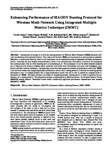
the paths with better metrics, but still distributes some load over other routes. Simulation results show that an un-equal cost multipath (LQDW) has about one-third the network load of minimum-cost multipath and unipath routing and a slightly higher delivery ratio in 100-node scenarios.
1
Delivery Ratio
0.8
0.6
R EFERENCES
0.4
0.2 LQMDW UNI LQDW
0 0
100
300 500 700 pause time (seconds)
Fig. 4.
900
Delivery Ratio
average path length is between 2.5 and 3.3 hops. The multipath protocols maintained between 1.2 and 1.5 multipaths per hop. In the 100-node scenarios, the delivery ratio in Fig. 4 is statistically equivalent between UNI, LQMDW, and LQDW, though LQDW has a slightly higher average. The network load in Fig. 6 shows that UNI and LQMDW have equivalent loads, but the un-equal cost multipath LQDW has a lower overall load, at times by a factor of 3. The CBR latency in Fig. 7 shows that LQDW has a slightly higher latency, but it is still statistically equivalent to UNI and LQMDW. The average path length is the same for all three protocols, between 4.3 hops and 5.5 hops. The extra two hops in path length compared to 50-node scenarios likely account for the greater difference between the min-hop protocols (UNI and LQMDW) and the un-equal cost protocol (LWDW). The multipath protocols in Fig. 8 maintain between 1.2 and 1.5 multipaths per hop. Interestingly, the un-equal cost multipath maintains fewer paths on average the equal-cost multipath. We have not analyzed the data to understand why that happens. VII. C ONCLUSION We argue that restricting multipath in ad hoc networks to disjoint paths is counter productive. By exploiting rich mesh connectivity, a network becomes more reliable and better amortizes the cost of on-demand path discovery over many links. In a review of the literature, there is no strong case for disjoint paths. Kleinrock’s argument for fixed routing is only under optimal capacity assignments in static networks. Using combinatorial analysis of a sample network, we illustrate how the reliability improves by adding more links. We adapt a combinatorial method to evaluate the s, tconnectedness lifetime of the sample network, and find that a mesh multipath topology has a significantly longer mean lifetime than a two disjoint path topology. In simulation, we compare a unipath, minimum cost multipath, and unequal cost multipath schemes. The unipath scheme uses one minimum cost path for routing. The minimum cost scheme uses all min-hop paths and distributes traffic based on next-hop link reliability. The unequal cost scheme distributes traffic based on a joint measurement of distance and link quality. To distribute traffic, we use a Boltzmann distribution which tends to select
[1] S. Nelakuditi and Z.-L. Zhang, “On selection of paths for multipath routing,” Lecture Notes in Computer Science, vol. 2092, pp. 170–184, 2001. [2] P. Baran, S. Boehm, and P. Smith, “On distributed communication,” RAND Corp., Santa Monica, CA, USA, Tech. Rep. 9, 1964. [3] L. Kleinrock, Communication nets: stocastic message flow and delay. New York: McGraw-Hill Book Company, 1964. [4] G. Ash and P. Chemouil, “20 years of dynamic routing in circuitswitched networks: looking backward to the future.” [Online]. Available: http://perso.rd.francetelecom.fr/chemouil/gcn ieee/DynRout20.pdf [5] J. Raju and J. J. Garcia-Luna-Aceves, “A new approach to on-demand loop-free multipath routing,” in IC3N’99. IEEE, Oct. 1999, pp. 522–7. [6] V. D. Park and M. S. Corson, “A highly adaptive distributed routing algorithm for mobile wireless networks,” in IEEE INFOCOM, Apr. 1997, pp. 1405–13 vol.3. [7] J. J. Garcia-Luna-Aceves, M. Mosko, and C. Perkins, “A new approach to on-demand loop free routing in ad hoc networks,” in PODC 2003, July 2003, pp. 53–62. [8] M. Mosko and J. J. Garcia-Luna-Aceves, “Loop-free routing using a dense label set in wireless networks,” in ICDCS 2004, Mar. 2004. [9] H. Rangarajan and J. Garcia-Luna-Aceves, “Using labeled paths for loop-free on-demand routing in ad hoc networks,” in MobiHoc, 2004. [10] S.-J. Lee and M. Gerla, “AODV-BR: backup routing in ad hoc networks,” in Proc. IEEE Conf. on Wireless Communications and Networking, Sept. 2000, pp. 1311–16 vol.3. [11] R. Dube, C. Rais, K. Wang, and S. Tripathi, “Signal stability based adaptive routing (SSA) for ad hoc mobile networks,” IEEE Personal Communication, Feb. 1997. [12] C.-K. Toh, “Associativity-based routing for ad hoc mobile networks,” Wireless Personal Communication, vol. 4, no. 2, pp. 103–139, 1997. [13] T. Goff, N. Abu-Ghazaleh, S. Phatak, and R. Kahvecioglu, “Preemptive routing in ad hoc networks,” in Mobile Computing and Networking, 2001, pp. 43–52. [14] M. Pearlman, Z. Haas, P. Sholander, and S. Tabrizi, “The impact of alternate path routing for load balancing in mobile ad hoc networks,” in Proc. ACM MobiHoc, 2000, pp. 3 –10. [15] K. Wu and J. Harms, “On-demand multipath routing for mobile ad hoc networks,” in Proc. EPMCC, 2001. [16] S. Roy, D. Saha, S. Bandyopadhyay, T. Ueda, and S. Tanaka, “Improving end-to-end delay through load balancing with multipath routing in ad hoc wireless networks using directional antenna,” in Proc. IWDC 2003: 5th International Workshop, LNCS v2918, Jan. 2003, pp. 225 – 234. [17] M. Marina and S. Das, “On-demand multipath distance vector routing in ad hoc networks,” in Proc. ICNP, 2001, pp. 14–23. [18] S.-J. Lee and M. Gerla, “Split multipath routing with maximally disjoint paths in ad hoc networks,” in IEEE ICC, 2001, pp. 3201–3205. [19] M. Mosko and J. Garcia-Luna-Aceves, “Ad hoc routing with distributed ordered sequences,” in submitted for publication, 2006. [20] L. J. Ford and D. Fulkerson, Flows in networks. Princeton, NJ, USA: Princeton University Press, 1962. [21] J. T. Moy, OSPF: anatomy of an Internet routing protocol. Reading, MA, USA: Addison-Wesley, 1998. [22] D. G. Cantor and M. Gerla, “Optimal routing in a packet-switched computer network,” IEEE Transactions on Computers, vol. C-23, no. 10, pp. 1062–9, Oct. 1974. [23] R. Gallager, “A minimum delay routing algorithm using distributed computation,” IEEE Trans. Comm., vol. COM-25, no. 1, pp. 73–75, 1977. [24] J. Suurballe, “Disjoint paths in a network,” Networks, vol. 4, pp. 125 – 145, 1974. [25] R. Ogier and N. Shacham, “A distributed algorithm for finding shortest pairs of disjoint paths,” in IEEE INFOCOM. IEEE, Apr. 1989, pp. 173–82 vol.1. [26] S.-N. Chiou and V. O. K. Li, “An optimal two-copy routing scheme in a communication network,” in IEEE INFOCOM, Mar. 1988, pp. 288–97.
10
5
LQMDW UNI LQDW
LQMDW UNI LQDW
4.5
8
4 Network Load
3.5 Hops
6
4
3 2.5 2 1.5
2
1 0.5
0 0
100
300 500 700 pause time (seconds)
Fig. 5.
900
0
Path hop count
1
300 500 700 pause time (seconds)
Fig. 6. 5
LQMDW UNI LQDW
0.9
900
Network Load
LQMDW UNI LQDW
4
0.8 Number Choices
0.7 Seconds
100
0.6 0.5 0.4 0.3
3
2
1
0.2 0.1
0 0
100
300 500 700 pause time (seconds)
Fig. 7.
900
Latency
[27] S.-N. Chiou and V. Li, “Diversity transmissions in a communication network with unreliable components,” in IEEE ICC, 1987, pp. 27.3.1 – 27.3.6. [28] A. Nasipuri, R. Castaeda, and S. R. Das, “Peformance of multipath routing for on-demand protocols in mobile ad hoc networks,” in ACM/Baltzer Mobile Networks and Applications (MONET) Journal, vol. 6, 2001, pp. 339–349. [29] C. Colbourn, The Combinatronics of Network Reliability. New York: Oxford University Press, 1987. [30] C. Perkins, E. Belding-Royer, and S. Das, “Ad hoc On-Demand Distance Vector (AODV) Routing,” RFC 3561 (Experimental), July 2003. [Online]. Available: http://www.ietf.org/rfc/rfc3561.txt [31] G. Grimmett and D. Stirzaker, Probability and Random Processes, 2nd ed. New York: Oxford University Press, 1992. [32] R. Feynman, Statistical Mechanics: A Set of Lectures. Redwood City, CA: Addison-Wesley, 1972. [33] D. Goldberg, “A note on Boltzmann tournament selection for genetic algorithms and population-oriented simulated annealing,” Complex Systems, vol. 4, pp. 445 – 460, 1990. [34] K. e. Fall and K. e. Varadhan, “The ns manual,” 2003, http://www.isi.edu/nsnam/ns/doc/index.html.
0
100
Fig. 8.
300 500 700 pause time (seconds)
Number of multipaths
900