George Tzagkarakis, Dimitris Milioris and Panagiotis Tsakalides. Department of Computer Science, ..... Dallas, Texas, USA. [14] A. Gurbuz, J. McClellan and V.
MULTIPLE-MEASUREMENT BAYESIAN COMPRESSED SENSING USING GSM PRIORS FOR DOA ESTIMATION George Tzagkarakis, Dimitris Milioris and Panagiotis Tsakalides Department of Computer Science, University of Crete & Institute of Computer Science - FORTH e-mail: {gtzag, milioris, tsakalid}@ics.forth.gr ABSTRACT Traditional bearing estimation techniques perform Nyquist-rate sampling of the received sensor array signals and as a result they require high storage and transmission bandwidth resources. Compressed sensing (CS) theory provides a new paradigm for simultaneously sensing and compressing a signal using a small subset of random incoherent projection coefficients, enabling a potentially significant reduction in the sampling and computation costs. In this paper, we develop a Bayesian CS (BCS) approach for estimating target bearings based on multiple noisy CS measurement vectors, where each vector results by projecting the received source signal on distinct over-complete dictionaries. In addition, the prior belief that the vector of projection coefficients should be sparse is enforced by fitting directly the prior probability distribution with a Gaussian Scale Mixture (GSM) model. The experimental results show that our proposed method, when compared with norm-based constrained optimization CS algorithms, as well as with single-measurement BCS methods, improves the reconstruction performance in terms of the detection error, while resulting in an increased sparsity. 1. INTRODUCTION Direction of arrival (DOA) estimation is a classic problem in the field of signal processing due to its numerous applications, from target tracking in a military environment to the localization of a mobile user in a smart home or a museum. Among the most prominent highresolution techniques, MUSIC [1] detects frequencies in a signal by performing an eigen-decomposition on the covariance matrix of the received signal samples. The algorithm assumes that the number of samples and frequencies are known, with an increasing accuracy as more samples are acquired, but at the cost of a high computational complexity. MVDR [2] is based on the minimization of the output power, subject to the constraint that the gain in the steering direction is unity. Classical MVDR beamforming techniques suffer from signal suppression in the presence of errors, such as the uncertainty in the look direction and array perturbations. In addition, all traditional DOA estimation techniques acquire the source signals by sampling them at Nyquist’s rate, which may result in high storage and bandwidth requirements in many modern sensing systems. In a typical scenario, a number of sensors capture signals transmitted from several sources. The received samples are then combined to estimate the position of the sources, either by exchanging them using in-network communications among sensors or by transmitting them to a fusion center (FC) with increased power This work was funded by the Greek General Secretariat for Research and Technology under Program ΠENE∆-Code 03E∆69 and by the Marie Curie TOK-DEV “ASPIRE” grant (MTKD-CT-2005-029791) within the 6th European Community Framework Program.
and processing capabilities. In untethered sensor arrays, the amount of transmitted information must be reduced as much as possible, since the communication cost dominates the power consumption. A critical observation is that the problem of DOA estimation in an environment with a number of sensors and much fewer sources presents an inherent sparsity in the space-domain. If we view the monitored field as a dense grid with the sensors and sources placed on the nodes of the grid, then each sensor can be associated with a vector with all of its components being zero except for those corresponding to the nodes of the grid where the sources are placed. Compressed sensing (CS) is a framework introduced recently for simultaneous sensing and compression enabling a potentially significant reduction in the sampling and computation costs at a sensing system with limited capabilities [4, 5]. Several CS methods have been proposed providing efficient sparse representations and reconstruction for the single-measurement vector (SMV) case. In particular, a signal having a sparse representation in a transform basis can be reconstructed from a vector containing a small number of projections onto a second, measurement basis that is incoherent with the first one. The property of asymmetry of the CS-based approaches is also a crucial point for the design of real-time sensing systems for DOA estimation, since the compression part is of very low complexity (simple linear projections), while the main computational burden is on the decompression part where increased processing capabilities and computational resources are available. On the other hand, the problem of sparse representation and reconstruction in the case of multiple-measurement vectors (MMV) in an over-complete dictionary is motivated by several inverse problems that arise in distinct fields, such as in astronomy [6] and medical imaging [7]. The corresponding noisy CS reconstruction problem is stated as follows: G = ΦW + H , (1) where G = [~g1 , . . . , ~gK ] ∈ RM ×K is the MMV matrix, Φ = ~1 , . . . , φ ~ N ] ∈ RM ×N (M < N ) is a random measurement ma[φ trix, W = [w ~ 1, . . . , w ~ K ] ∈ RN ×K is the weight vectors matrix and H = [~ η1 , . . . , ~ ηK ] ∈ RM ×K is the noise matrix. Each sparse weight vector is the transform-domain equivalent of the corresponding original time-domain signal, f~i = Ψi w ~ i , i = 1, . . . , K, where the columns of Ψi ∈ RN ×N correspond to the transform basis functions. In general, each f~i is considered sparse on a different basis Ψi . For K = 1, the problem is reduced to the standard CS reconstruction using a single measurement vector. Several CS methods have been introduced recently that give an estimate of W satisfying (1) by solving a norm-based constrained optimization problem [8, 9, 10]. On the other hand, the work presented in [11] develops a reconstruction method in a Bayesian framework, by modelling the prior belief that the majority of the rows of W will be zero, due to the assumption for a joint sparsity structure,
by employing a zero-mean Gaussian distribution on the norm of each individual row. The Bayesian framework provides the critical advantage that we obtain not only a point estimate of the signal, as the norm-based methods do, but also a confidence interval, which can be employed to select appropriately the future measurements such as to reduce the uncertainty [12]. Often, we are interested in reconstructing a single original signal from multiple measurements. This is the case in DOA estimation using a sensor network, where we try to reconstruct the vector of sources’ positions using multiple observations of it. For this purpose, in this paper we generalize our related work [13] for the case of multiple measurements. The paper is organized as follows: In Section 2, the statistical signal model is presented, while in Section 3 the proposed Bayesian CS reconstruction algorithm using multiple measurement vectors is described. In Section 4, we compare the performance of the proposed approach with other state-of-the-art CS recovery methods. Finally, we conclude in Section 5. 2. STATISTICAL SIGNAL MODEL Although in the present DOA estimation scenario we consider a 2-D space, the procedure is generalized to a higher dimensional space in a straightforward way. In our setting we consider a field consisting of a linear array of K sensors and L sources. Each sensor receives a suP perposition of the time-domain source signals, f (t) = L l=1 fl (t). Given these received signals, the goal is to determine the DOA of each source. We also assume that the sensor positions are known in advance, {~ni = [xi , yi ]T }K i=1 . The i-th sensor receives a timedelayed and attenuated version of the superimposed source signal f (t), given by: ¡ ¢ wi (t) = αf t + ∆i (θf ) − (R/c) , (2) where α is the attenuation, θf are the unknown azimuths and ∆i (θf ) is the relative time-delay at the i-th sensor of the signal transmitted at θf . In the following, we ignore the attenuation and assume that the Rc term is known, or constant across the array (far-field assumption), where R is the sensor-source range and c is the speed of the propagating wave in the medium. Motivated by a recent work [14], the azimuth space is discretized by forming a finite set of angles B = {θ1 , θ2 , . . . , θN } where N determines the resolution. Let ~b denote the sparse vector, which selects elements from B. A non-zero component ~bj > 0 indicates the presence of a source at an azimuth of θj . For L = 1 the sparsity pattern vector ~b has only one non-zero entry and thus, this is the case of the highest possible sparsity. In particular, the angle space is discretized in 180 points, which corresponds to a resolution of 1 degree. Doing so, the sparsifying transform matrices {Ψi }K i=1 will be of dimension P × 180 (P À 180), where P is the number of data samples per source, with their columns containing the received time-delayed signals from each potential source location (elements of B). Besides, the i-th sensor is associated with a distinct random measurement matrix Φi ∈ RM ×P , where M is the number of measurements per sensor. The bearing sparsity pattern vector ~b is related linearly to the received signal at the i-th sensor via the expression w ~ i = Ψi~b . The corresponding set of measurement vectors for the K sensors in the general noisy case is given by: ˜ i~b + ~ ~gi = Φi w ~i + ~ ηi = Φ ηi , i = 1, . . . , K (3) M ˜ where Φi = Φi Ψi and ~ ηi ∈ R is a noise vector with unknown variance ση2 . In our case, the set {Φi }K i=1 contains matrices with independent and identically distributed (i.i.d.) Gaussian entries. Such
matrices are incoherent with any fixed transform matrix Ψ with high probability (universality property) [5]. Also notice that this model differs from the one given by (1) in that distinct measurement matrices are used on a single weight vector, instead of a matrix. Thus, given the matrix G = [~g1 , . . . , ~gK ] containing the multiple measurement vectors and the measurement matrices {Φi }K i=1 the reconstruction problem reduces to estimating the sparse vector ~b. In [6], this problem is solved by employing a norm-based constrained optimization approach. The reconstruction can be also recast as an SMV problem and solved with one of the many normbased CS approaches as follows: ~ˆb = arg min k~bk1 s.t. kG − ΦΨ~bk < ² , (4) where Ψ = [Ψ1 , . . . , ΨK ]T , Φ = diag(Φ1 , . . . , ΦK ) and ² is the noise level. On the other hand, when the inversion of CS measurements is treated from a Bayesian perspective, then, given the prior belief that w ~ i is L-sparse in basis Ψi (that is, only L of ~b’s components have “significant” amplitude) and the MMV matrix G, the objective is to formulate a posterior probability distribution for ~b. This improves the accuracy over the point estimate given by a norm-based approach and provides confidence intervals (error bars) in the estimation of DOA’s, which can be used to guide the optimal design of additional CS measurements with the goal of reducing the estimation uncertainty. 3. MULTIPLE-MEASUREMENT BCS RECONSTRUCTION USING GSM PRIORS In this Section, we extend our work in [13] by incorporating the set of multiple measurement vectors in the reconstruction of ~b. Under the assumption of zero-mean Gaussian noise vectors with the same variance ση2 , we obtain the following Gaussian likelihood model for the measurement vector ~gi , i = 1, . . . , K, ¡ 1 ¢ ˜ i~bk . p(~gi |~b, ση2 ) = (2πση2 )−M/2 · exp − 2 k~gi − Φ 2ση
(5)
As mentioned above, the goal is to seek a full posterior density function for ~b and ση2 . The proposed extension consists in modeling directly the prior distribution of ~b with a heavy-tailed density, which promotes its sparsity, since it is suitable for modeling highly impulsive signals. In particular, we model the prior distribution of ~b by means of a Gaussian Scale Mixture (GSM). Definition 1 A vector ~b is called a GSM (in RN ) with underlying √ ~ iff it can be written in the form ~b = A V ~, Gaussian vector V ~ = (V1 , V2 , . . . , VN ) where A is a positive random variable and V is a zero-mean Gaussian random vector, independent of A, with covariance matrix Σ. The assumption of independence yields a diagonal covariance ma2 trix Σ = diag(σ12 , . . . σN ). From Definition 1, the density of ~b conditioned on the variable A is a zero-mean multivariate Gaussian given by, exp(− 21~bT (AΣ)−1~b) , (6) p(~b|A) = (2π)N/2 |AΣ|1/2 where | · | denotes the determinant of a matrix. From (6), we obtain the following simple expression for the maximum likelihood (ML) estimate of the variable A, ¡ ¢ ˆ ~b) = ~bT Σ−1~b /N . A( (7)
Assuming that the noise variance ση2 , the value of A and the covariance matrix Σ have been estimated, given the CS measurement ˜ i , the posterior density of ~b is given by vector ~gi and the matrix Φ Bayes’ rule p(~gi |~b, ση2 )p(~b|A, Σ) p(~b|~gi , A, Σ, ση2 ) = , (8) p(~gi |A, Σ, ση2 ) which is a multivariate Gaussian distribution with a mean vector µ ~i and a covariance matrix Pi , given by µ ~i
=
Pi
=
˜ Ti ~gi , ση−2 Pi Φ ˜ Ti Φ ˜ i + M)−1 , i = 1, . . . , K (ση−2 Φ
(9) (10)
2 −1 ) ). diag((Aσ12 )−1 , . . . , (AσN
The presence of the where M = scale parameter A in the proposed GSM-based BCS method provides an additional degree of freedom, which may result in a more accurate modeling of the true sparsity of the signal of interest, as well as the noise component, when compared with previous BCS approaches [12, 15], as the experimental results reveal. The problem of estimating the sparse vector ~b reduces to estimating the unknown model parameters A, Σ, ση2 , by combining type-II ML estimations from the K measurement vectors. For this purpose, we estimate the unknown parameters ση2 , {σj2 }N j=1 iteratively by employing a modified version of the marginal log-likelihood function used in [13]. In particular, we have to incorporate explicitly the information provided by the matrix G. We do this by summing up the contributions of the individual measurement vectors ~gi , resulting in the following log-likelihood function: K X L(ση2 , {σj−2 }N ) = log[p(~gi |A, ση2 , {σj−2 }N j=1 j=1 )] i=1 K
=−
K
X X T −1 ¤ 1£ KM log(2π) + log(|Ci |) + ~gi Ci ~gi ,(11) 2 i=1 i=1 2
σ ˜ i ΣΦ ˜ Ti . It is clear from (11) that the scaling where Ci = Aη I + Φ factor of 1/A plays an important role in the estimation process, since it controls the heavy-tailed behavior of the diagonal elements of M and consequently of the covariance matrices {Pi }K i=1 , and thus, the sparsity of the estimated vector ~b which depends on the corresponding mean vectors {~ µi }K i=1 , as we will see in the subsequent analysis. The addition and deletion of candidate basis functions (columns of ˜ i }K {Φ i=1 ) is performed with the goal to monotonically increase the marginal likelihood. Following a similar incremental procedure as the one used in [13], the computational cost for updating the most “expensive” quantities of (11), namely the determinants {|Ci |}K i=1 K and the inverses {C−1 i }i=1 , is reduced significantly. After some algebraic manipulation, we can see that the marginal likelihood is decoupled in two terms, as follows: 2 −2 N −2 L(ση2 , {σj−2 }N j=1 ) = L(ση , {σj }j=1,j6=j 0 ) + l(σj 0 ) ,
(12)
where the first term depends on all except for the j 0 -th variance, while the second term depends only on the j 0 -th variance. This decoupling also accelerates the updating of (11). In particular, l(σj−2 0 ) is given by: K 2 ¢i qi,j 0 1 hX ¡ −2 l(σj−2 log(σj−2 0 ) = 0 ) − log(σj 0 + si,j 0 ) + −2 2 i=1 σj 0 + si,j 0 (13) ~ ~˜ 0 ~˜T ~˜ 0 −1 0 where si,j 0 = φ˜Ti,j 0 C−1 φ and q = φ C ~ g , with φ i,j i,j i,j 0 i,−j 0 i i,−j 0 i,j ˜ i and Ci,−j 0 is equal to Ci with the denoting the j 0 -th column of Φ ~ contribution of j 0 -th basis vector φ˜i,j 0 removed.
3.1. Estimation of the sparse vector ~b The fact that all covariance matrices {Pi }K i=1 depend on the same model parameters (ση2 , M) means that the algorithm will converge to a common set of indices indicating the significant basis vectors ˜ i. which are used from each measurement matrix Φ Each iteration of the proposed algorithm results in K multivariate Gaussians with parameters (~ µi , Pi ) given by (9)-(10) by employing the model parameters estimated by maximizing (13). Working in a Bayesian framework, we are interested in combining these Gaussians in a single “best” representative, which will be then considered to be the estimation of the sparse vector ~b. For this purpose, a clustering method exploiting the statistical assumptions made in this work must be used. The standard k-means techniques exploit only first-order moments and they also assume that each input is a sample drawn from one of k distributions (here Gaussians). However, in the proposed method we have to incorporate the information of the second-order moments (covariance matrices), since they represent the heavy-tailed behavior of ~b, which is crucial for achieving an increased sparsity and also we are interested in clustering a set of distributions (and not a set of samples) into a single best representative. For this purpose, we employ a differential entropic clustering (DEC) of the K multivariate Gaussians [16] and the best representative (~ µ∗ , P∗ ) is defined as the multivariate Gaussian that minimizes the total differential entropy with respect to the K Gaussians. Thus, at the end of each iteration the estimated value of ~b is defined as ~ˆb ≡ µ ~ ∗ , with µ ~∗ =
K X i=1
ci µ ~ i , P∗ =
K X ¡ ¢ ci Pi + (~ µi − µ ~ ∗ )(~ µi − µ ~ ∗ )T (14) i=1
where ci are weights, which we choose to be equal to 1/K. It is also important to note that the update of A from (7) is carried out by substituting ~b with the estimated µ ~ ∗. 4. EXPERIMENTAL RESULTS In this section, we compare the performance of the proposed MMV reconstruction scheme (M-BCS-GSM) with the SMV methods BCS, BCS-GSM [12, 13], as well as with some state-of-the-art normbased optimization schemes: 1) Gradient Projection for Sparse Reconstruction (GPSR), 2) Basis Pursuit (BP), 3) Stagewise Orthogonal Matching Pursuit (StOMP), 4) `1 -norm minimization using the primal-dual interior point method (L1EQ-PD) and 5) Smoothed `0 (SL0)1 . The time delay between each potential source position and the sensor is computed for c = 340 m/s with a sampling frequency fs = 500 Hz, while the source signals are generated by drawing 512 samples from a Gaussian distribution N (0, 1). Besides, the sensor array consists of 5 sensors placed at a distance of 10o (on the grid) from each other. The SNR at the leftmost sensor is equal to 20 dB and it reduces at 1.5 dB from sensor to sensor as we are moving on the right side of the array. We illustrate the efficiency of the proposed method for estimating DOA’s in two test cases: 1) presence of a single source placed at 54o and 2) presence of two sources with small angular separation at 41o and 44o , respectively, in order to evaluate the discrimination capability of the several CS 1 For the implementation of BCS and methods 1)-5) we used the MATLAB codes included in the packages: http://sparselab.stanford. edu/, http://www.lx.it.pt/˜mtf/GPSR, http://www.acm. caltech.edu/l1magic, http://ee.sharif.ir/˜SLzero.
Percentage of successful detections (%)
reconstruction methods. In each case the results are averaged over 100 Monte-Carlo runs for a varying number of measurements per sensor, M ∈ {10, 15, 20, 25, 30}. Fig. 1(a) shows the average number of successful source detections of the source at 54o , where a detection is characterized as successful if it recovers all the sources. As we can see, the proposed method results in the highest detection performance, which increases as M increases. Its “centralized” SMV analogue (BCS-GSM) along with the norm-based methods GPSR and L1EQ-PD also perform well, but by employing many more basis functions, as shown in Fig. 1(b). This significant increase of the sparsity achieved by the proposed method is very important for resource preservation in a sensor network application. (a) 100
GPSR BP STOMP L1EQ−PD SL0 BCS BCS−GSM M−BCS−GSM
80 60 40 20 0 10
15
20
25
30
(b) # of significant basis vectors
200 150 100 50 0 10
12
14
16
18
20
22
24
26
28
30
Number of measurements (M)
Fig. 1. DOA estimation performance for one source (54o ).
Percentage of successful detections (%)
Fig. 2(a) shows the average number of successful source detections for the case of two sources. As in the single source case, the proposed method results in the highest detection performance for M > 15, with the BCS-GSM and L1EQ-PD methods following closely. However, as Fig. 2(b) shows, the proposed method results again in an important increase of the sparsity (e.g., at the order of 80% for M = 30 in comparison with the BCS-GSM and at an even higher order when compared with the other methods). (a) 100
GPSR BP STOMP L1EQ−PD SL0 BCS BCS−GSM M−BCS−GSM
80 60 40 20 0 10
15
20
25
30
(b) # of significant basis vectors
200 150 100 50 0 10
12
14
16
18
20
22
24
26
28
30
Number of measurements (M)
Fig. 2. DOA estimation performance for two sources (41o , 44o ).
5. CONCLUSIONS AND FUTURE WORK In this work, we described a method for CS reconstruction in a Bayesian framework using multiple measurement vectors, generated by projecting a single (sparse) vector on multiple measurement matrices. The experimental results revealed a critical property of the proposed M-BCS-GSM approach when compared with other CS reconstruction methods. In particular, we showed that the M-BCSGSM implementation achieves a higher reconstruction performance, while using much fewer basis functions and thus, resulting in an increased sparsity. In the present work, we did not make any assumption for the probability density function of the scaling factor A of the GSM. In future work, we are interested in posing a heavy-tailed distribution on the random variable A. In particular, when A follows an α-stable distribution, then, the GSM is reduced to a sub-Gaussian model. We expect that the characteristic exponent which appears in the α-Stable distribution will provide further control on the sparsity of the weight vector. 6. REFERENCES [1] P. Stoica and A. Nehorai, “MUSIC, Max. Likelihood, and Cramer-Rao Bound,” IEEE Trans. Acoustics, Speech & Sig. Proc., Vol. 37, No. 5, pp. 720–741, 1989. [2] H. Cox et al., “Robust Adaptive Beamforming,” IEEE Trans. Acoustics, Speech & Sig. Proc. Vol. 35, No. 10, pp. 1365–1377, 1987. [3] D. Johson and D. Dudgeon, “Array Signal Processing: Concepts and Techniques,” New Jersey: PTR Prentice-Hall, Inc., 1993. [4] E. Cand` es et al., “Robust uncertainty principles: Exact signal reconstruction from highly incomplete frequency information,” IEEE Trans. Inform. Theory, Vol. 52, No. 2, pp. 489–509, Feb. 2006. [5] D. L. Donoho, “Compressed Sensing,” IEEE Trans. Inf. Theory, Vol. 52, No. 4, pp. 1289–1306, Apr. 2006. [6] J. Bobin et al., “Compressed Sensing in Astronomy,” IEEE J. Sel. Topics in Sig. Proc., Vol. 2, No. 5, pp. 718–726, Oct. 2008. [7] M. Lustig, D. Donoho and J. Pauly, “Sparse MRI: The application of compressed sensing for rapid MR imaging,” Magn. Reson. Med., Vol. 58, No. 6, pp. 1182–1195, 2007. [8] J. Chen and X. Huo, “Sparse representations for multiple measurement vectors (MMV) in an overcomplete dictionary,” in Proc. IEEE Int. Conf. Acoustics, Speech, Signal Proc., pp. 257–260, Mar. 2005. [9] S. Cotter, B. Rao, K. Engan and K. Kreutz-Delgado, “Sparse solutions to linear inverse problems with multiple measurement vectors,” IEEE Trans. Signal Proc., Vol. 53, No. 7, pp. 2477–2488, Jul. 2005. [10] J. Tropp, A. Gilbert and M. Strauss, “Algorithms for simultaneous sparse approximation. Part I: Greedy pursuit,” EURASIP J. Signal Proc., Vol. 86, pp. 572–588, Apr. 2006. [11] D. Wipf and B. Rao, “An Empirical Bayesian Strategy for Solving the Simultaneous Sparse Approximation Problem,” IEEE Trans. Signal Proc., Vol. 55, No. 7, pp. 3704–3716, July 2007. [12] S. Ji, Y. Xue and L. Carin, “Bayesian Compressive Sensing,” IEEE Trans. on Signal Proc., Vol. 56, No. 6, pp. 2346–2356, June 2008. [13] G. Tzagkarakis and P. Tsakalides, “Bayesian Compressed Sensing Imaging using a Gaussian Scale Mixture,” in Proc. IEEE Int. Conf. on Acoust., Speech and Sig. Proc. (ICASSP’2010), Mar. 14–19, 2010, Dallas, Texas, USA. [14] A. Gurbuz, J. McClellan and V. Cevher, “A compressive beamforming method,” Proc. IEEE Int. Conf. on Acoust., Speech and Sig. Proc. (ICASSP’08), Mar. 31–Apr. 4, 2008, Las Vegas, USA. [15] P. Schniter et al., “Fast Bayesian Matching Pursuit,” Proc. Workshop on Information Theory & Applications, La Jolla, CA, Jan. 2008. [16] J. Davis and I. Dhillon, “Differential Entropic Clustering of Multivariate Gaussians,” Adv. in Neural Inf. Proc. Systems, 2006.