Multiscale simulations of tropospheric chemistry in the eastern Pacific ...

JOURNAL OF GEOPHYSICAL RESEARCH, VOL. 109, D23S11, doi:10.1029/2004JD004513, 2004

Multiscale simulations of tropospheric chemistry in the eastern Pacific and on the U.S. West Coast during spring 2002 Youhua Tang,1 Gregory R. Carmichael,1 Larry W. Horowitz,2 Itsushi Uno,3 Jung-Hun Woo,1 David G. Streets,4 Donald Dabdub,5 Gakuji Kurata,6 Adrian Sandu,7 James Allan,8 Elliot Atlas,9 Franck Flocke,9 Lewis Gregory Huey,10 Roger O. Jakoubek,11 Dylan B. Millet,12 Patricia K. Quinn,13 James M. Roberts,11 Douglas R. Worsnop,14 Allen Goldstein,12 Stephen Donnelly,9 Sue Schauffler,9 Verity Stroud,9 Kristen Johnson,9 Melody A. Avery,15 Hanwant B. Singh,16 and Eric C. Apel9 Received 5 January 2004; accepted 10 March 2004; published 9 July 2004.

[1] Regional modeling analysis for the Intercontinental Transport and Chemical

Transformation 2002 (ITCT 2K2) experiment over the eastern Pacific and U.S. West Coast is performed using a multiscale modeling system, including the regional tracer model Chemical Weather Forecasting System (CFORS), the Sulfur Transport and Emissions Model 2003 (STEM-2K3) regional chemical transport model, and an off-line coupling with the Model of Ozone and Related Chemical Tracers (MOZART) global chemical transport model. CO regional tracers calculated online in the CFORS model are used to identify aircraft measurement periods with Asian influences. Asian-influenced air masses measured by the National Oceanic and Atmospheric Administration (NOAA) WP-3 aircraft in this experiment are found to have lower DAcetone/DCO, DMethanol/DCO, and DPropane/DEthyne ratios than air masses influenced by U.S. emissions, reflecting differences in regional emission signals. The Asian air masses in the eastern Pacific are found to usually be well aged (>5 days), to be highly diffused, and to have low NOy levels. Chemical budget analysis is performed for two flights, and the O3 net chemical budgets are found to be negative (net destructive) in the places dominated by Asian influences or clear sites and positive in polluted American air masses. During the trans-Pacific transport, part of gaseous HNO3 was converted to nitrate particle, and this conversion was attributed to NOy decline. Without the aerosol consideration, the model tends to overestimate HNO3 background concentration along the coast region. At the measurement site of Trinidad Head, northern California, high-concentration pollutants are usually associated with calm wind scenarios, implying that the accumulation of local pollutants leads to the high concentration. Seasonal variations are also discussed from April to May for this site. A high-resolution nesting simulation with 12-km horizontal resolution is used to study the WP-3 flight over Los Angeles and surrounding areas. This nested simulation significantly improved the predictions for emitted and secondary generated species. The difference of photochemical behavior between the coarse (60-km) INDEX TERMS: and nesting simulations is discussed and compared with the observation. 0317 Atmospheric Composition and Structure: Chemical kinetic and photochemical properties; 0365 Atmospheric Composition and Structure: Troposphere—composition and chemistry; 0368 Atmospheric 1

Center for Global and Regional Environmental Research, University of Iowa, Iowa City, Iowa, USA. 2 Geophysical Fluid Dynamics Laboratory, NOAA, Princeton, New Jersey, USA. 3 Research Institute for Applied Mechanics, Kyushu University, Fukuoka, Japan. 4 Decision and Information Sciences Division, Argonne National Laboratory, Argonne, Illinois, USA. 5 Department of Mechanical and Aerospace Engineering, University of California, Irvine, California, USA. 6 Department of Ecological Engineering, Toyohashi University of Technology, Toyohashi, Japan. Copyright 2004 by the American Geophysical Union. 0148-0227/04/2004JD004513

7 Department of Computer Science, Virginia Polytechnic Institute and State University, Blacksburg, Virginia, USA. 8 Department of Physics, University of Manchester Institute of Science and Technology, Manchester, UK. 9 National Center for Atmospheric Research, Boulder, Colorado, USA. 10 School of Earth and Atmospheric Sciences, Georgia Institute of Technology, Atlanta, Georgia, USA. 11 Aeronomy Laboratory, NOAA, Boulder, Colorado, USA. 12 Department of Environmental Science, Policy, and Management, University of California, Berkeley, California, USA. 13 Pacific Marine Environmental Laboratory, NOAA, Seattle, Washington, USA. 14 Aerodyne Research Inc., Billerica, Massachusetts, USA. 15 NASA Langley Research Center, Hampton, Virginia, USA. 16 NASA Ames Research Center, Moffett Field, California, USA.

D23S11

1 of 25

D23S11

TANG ET AL.: MULTISCALE SIMULATIONS OF TROPOSPHERIC CHEMISTRY

D23S11

Composition and Structure: Troposphere—constituent transport and chemistry; 3337 Meteorology and Atmospheric Dynamics: Numerical modeling and data assimilation; KEYWORDS: chemical transport model, nesting simulation, atmospheric photochemistry Citation: Tang, Y., et al. (2004), Multiscale simulations of tropospheric chemistry in the eastern Pacific and on the U.S. West Coast during spring 2002, J. Geophys. Res., 109, D23S11, doi:10.1029/2004JD004513.

1. Introduction [2] During April and May 2002 the Intercontinental Transport and Chemical Transformation 2002 (ITCT 2K2) experiment studied the air mass characteristics over the eastern Pacific and the U.S. West Coast. National Oceanic and Atmospheric Administration (NOAA) WP-3 aircraft and surface measurements were performed with the objective of characterizing the Asian inflow signal and its impact on regional air quality. During this period, air masses impacted by Asian emissions are transported to the eastern Pacific by the midlatitude prevailing westerlies. The longdistance transport of Asian pollutants to the west coast of North America has been studied by many researchers, such as Jaffe et al. [1999] and Kotchenruther et al. [2001]. Jacob et al. [1999] discussed the impact of Asian emissions variation on North America air quality using a global model. The strength of the Asian influence on North America was shown to depend on the Asian emission strength and the transport efficiency over the Pacific Ocean. Asian emissions are composed of anthropogenic (including biofuel) sources, biomass burning, and volcanic activity. Woo et al. [2003] estimated the biomass-burning emission during the spring 2001. Carmichael et al. [2003a, 2003b] studied the features of Asian outflow over the west Pacific and used aircraft measurements and model results to evaluate the emission estimations by Streets et al. [2003a, 2003b]. Yienger et al. [2000] described the Asian pollutant transport to North America using CO as the criteria. The trans-Pacific transport of aerosol is also an important issue. During springtime Asian dust storms become active, and dust can be transport to the eastern Pacific and North America [Uno et al., 2001; VanCuren and Cahill, 2002]. However, during the ITCT 2K2 experiment the influence of Asian dust on North American was not significant. [3] To study the transport and chemistry of trace gases and aerosols across the northern Pacific, we used a regional chemical transport model. Regional models have an advantage over global models in their ability to use finer resolutions in the analysis, but have the disadvantage of requiring lateral boundary conditions. In this study the lateral boundary conditions were established using a multiscale modeling system with nested models. Nesting techniques can help in the analysis from two sides: introducing external influences for relatively long-lived transported species, such as CO or O3 [Langmann et al., 2003], and by considering high-resolution emissions for short-lived species, such as NOx or SO2 [Tang, 2002]. High-resolution emissions can more accurately resolve near-source concentrations, and better estimate photochemical budgets [Tang, 2002]. [4] In this paper, the multiscale model is used to help analyze aircraft and surface measurements obtained during the ITCT 2K2 experiment. In the following section the details of the model are presented. In section 3 Asian tracer

information calculated by the model is used to classify the aircraft observations into those observations with large and small Asian signals, which are then subsequently used to help quantify observed characteristics of Asian air masses over the eastern Pacific. Specific characteristics of individual aircraft flights are analyzed in section 4, where the multiscale model system is used to study the photochemistry in air masses over the eastern Pacific as aged air masses interact with emissions from North America. The WP-3 flight on 13 May over Los Angeles is analyzed as an example of the effect of model resolution on model predictions. The effect of aerosols on nitrate partitioning is presented in section 5. Results from a fine-scale nesting simulation of the flight around Los Angeles are presented in section 6. A mission-wide perspective of the performance of the model comprises section 7. Analysis of the Trinidad Head observations is presented in section 8.

2. Model System [5] Characterizing the Asian influence on the chemistry of the eastern Pacific is a challenge as trace species are diluted during their trans-Pacific transport, which makes it difficult to distinguish them from background conditions. These air masses also mix with local sources as they move inland. To efficiently consider these processes, a multiscale model system was established. This model system includes the Model of Ozone and Related Chemical Tracers (MOZART) global chemical transport model [Horowitz et al., 2003], the intercontinental chemical tracer model Chemical Weather Forecasting System (CFORS) [Uno et al., 2003], and a nested regional chemical transport model, Sulfur Transport and Emissions Model 2003 (STEM-2K3) [Tang et al., 2004]. The model domains are shown in Figure 1. [6] CFORS is an online tracer model [Uno et al., 2003] coupled with the RAMS regional meteorological model. In this application, CFORS was driven by NCEP reanalysis for postanalysis and AVN data for forecasting uses. CFORS treats chemical species as tracers assuming linear consumption. For example, NOx tracer in CFORS decays with a firstorder rate: d ½NOx ¼ kNOx ½NOx ; dt

ð1Þ

where kNOx is a fixed value. In CFORS, we define a conservative NOy (total odd nitrogen species) tracer that can be transported without loss, and assume that this NOy tracer has the same emission source as NOx. Under this assumption, the NOx age can be derived from equation (1): TNOx ¼ knox ln NOy =½NOx :

ð2Þ

This equation allows for the online calculation of the averaged NOx age when air masses from different sources

2 of 25

D23S11


D23S11

Figure 1. Model domains, NOAA WP-3 flight paths (colored lines), and estimated CO emissions on the various domains. See color version of this figure at back of this issue. mix together. This NOx age represents a combined result of transport time, diffusion, and NOx source intensities. With the same method we also define a volatile organic compound (VOC) age using ethane as an indicator that is related to ethane emission and decay rate. In this study, the decay rates used in CFORS for CO, SO2, NOx and ethane were 2.22 107, 2.78 106, 9.26 106, and 1.25 107 s1, respectively. [7] CO is one of the primary tracers in CFORS and is used to help classify emission source types and regions. In this study CO was parsed into: Asian anthropogenic, biomass burning (BB), Mexico, Canada, California, Washington-Oregon, and the rest of the United States. These regional CO tracers can be used to help determine the air mass properties and its mixing state. During the ITCT 2K2 field campaign, forecast products for these tracers were also used for flight planning. It is important to note that these CO tracers in CFORS do not yield a total CO value that can be quantitatively compared to observed values because they represent primary CO only. The CFORS analysis does not

consider CO that arises from methane and nonmethane hydrocarbon oxidation. Furthermore, the background levels were set to zero. In this paper, CFORS tracer model for ITCT 2K2 used a domain with 100 42 grids with a 200-km horizontal resolution (Figure 1), which covers east Asia, the northern Pacific Ocean, and most of North America. [8] Comprehensive chemistry and transport interactions are calculated by the STEM-2K3 regional chemical transport model, which is a further development of the STEM2K1 model [Tang et al., 2003a; Carmichael et al., 2003a] that includes the SAPRC-99 gaseous mechanism [Carter, 2000] and an explicit photolysis rate solver (the online NCAR Tropospheric Ultraviolet-Visible (TUV) radiation model, Madronich and Flocke [1999]). The main improvement of STEM-2K3 over STEM-2K1 is that the former also includes an aerosol thermodynamics module, Simulating Composition of Atmospheric Particles at Equilibrium (SCAPE II) [Kim et al., 1993a, 1993b; Kim and Seinfeld, 1995], for calculating gas-particle equilibrium concentrations among inorganic aerosol ions and their gaseous

3 of 25


D23S11

D23S11

Table 1. The 17 Vertical Layers (Over the Sea Surface) Used in CFORS and STEM-2K3 and CO Background Profile in the Eastern Pacific Vertical Layers Altitude, km CO, ppbv

1

2

3

4

5

6

7

8

9

10

11

12

13

14

15

16

17

0.075 120

0.24 120

0.44 120

0.68 120

0.96 120

1.3 120

1.7 120

2.2 110

2.8 110

3.5 110

4.4 110

5.4 108

6.6 105

8.1 105

9.8 98

11.6 85

13.4 80

precursors. Tang et al. [2004] described the framework of STEM-2K3 and its performance during the Transport and Chemical Evolution over the Pacific (TRACE-P) experiment [Jacob et al., 2003] and Asian Pacific Regional Aerosol Characterization Experiment (ACE-Asia). In this paper, the analysis includes inorganic aerosols in 4 size bins (in diameter): 0.1– 0.3 mm, 0.3– 1.0 mm, 1.0– 2.5 mm, and 2.5– 10 mm (referred to as bins 1 – 4, respectively). Daily Total Ozone Mapping Spectrometer (TOMS) data were used to calculate the model’s overtop ozone column needed in the photolysis calculations using the TUV module. [9] The primary domain for STEM-2K3 covers the U.S. West Coast and eastern Pacific with a 60-km horizontal resolution (Figure 1). Another RAMS model run in this domain was used to drive STEM-2K3. To better reflect the influence of more local sources, such as during the flight over the Los Angeles basin, a higher resolution is necessary. Here a nested domain with a nesting ratio of 1:5 (Figure 1) was used. The nested STEM-2K3 was driven by meteorology interpolated from the RAMS 60-km predication. The change in resolution affects the emission intensity. For example, Figure 1 shows that CO emission rate in Los Angeles ranges from 150 to 300 mole/h/km2 represented in the domain of 200-km resolution, is over 1500 mole/h/km2 in the 60-km domain, and greater than 3000 mole/h/km2 (peak value) with 12-km resolution. Tang [2002] discussed how model resolution affected O3 and NOx predications, and photochemical correlations through for the TRACE-P and ACE-Asia experiments. 2.1. Lateral Boundary Conditions [10] The MOZART global model was used to provide lateral boundary conditions for the STEM-2K3 primary 60-km domain (Figure 1) applications. The lateral boundary and top boundary conditions of STEM-2K3 for all species except CO were interpolated to the primary 60-km domain from the MOZART model results produced using NCEP winds. Because of the uncertainties in the CO emission inventories the global model tends to quantitatively underestimate CO in the midlatitudes and altitudes. The ITCT 2K2 aircraft observations showed that CO had a stable background concentration over the eastern Pacific, and CO contributions from various sources were mostly represented by enhancements above background. In this paper, we set the boundary condition of STEM-2K3 for CO to the background CO (shown in Table 1) plus a perturbation calculated as the total tracer CO from the CFORS model. The boundary values above the flight altitude of the WP-3 were obtained using the observations by the NASA DC-8 aircraft during the TRACE-P experiment. Table 1 also shows the model vertical layers used in CFORS and STEM-2K3, defined in the midpoint of the RAMS sigma-z layers [Pielke et al., 1992]. The nested 12-km domain has the same vertical layers as the 60-km primary domain, and

the lateral boundary conditions were also interpolated from the 60-km domain. 2.2. Emissions [11] Emission data used in this study came from various sources. The basic strategy to develop the assembled emissions inventory was to use global-scale emissions inventories as background/lower quality assurance information, and to supplement these with more comprehensive/ higher-quality regional-scale emissions data for Asia and North America regions. The Asian anthropogenic emissions were based on the estimate of Streets et al. [2003a, 2003b]. Biomass-burning emissions for Southeast Asia were based on April-averaged Asian BB emissions for the base year of 2001 [Woo et al., 2003]. Emissions in the United State and Canada were based on the USEPA 1996 inventory. Mexican emissions came from Kuhns et al. [2001]. The ship emissions for CO, SO2 and NOx were based on the inventory of Corbett et al. [1999], and aviation emissions were taken from EDGAR [Olivier et al., 1996]. Lightning NOx emissions were diagnosed from the meteorological model according to deep convective intensities [Pickering et al., 1998]. Emissions for all other regions in the 200-km domain came from Global Emissions Inventory Activities (GEIA) inventory http://geiacenter.org/). Biogenic emissions for the regions other than the United States come from GEIA [Guenther et al., 1995]. MOZART global model has it own emission [Horowitz et al., 2003], which is mainly based on the EDGAR inventory [Olivier et al., 1996]. [12] For simulating pollutant recirculation from the western U.S. into the Pacific Ocean and propagation from the West Coast inland, we used U.S. EPA emission databases and more detailed allocation procedures. For example, the emission data for the nested 12-km domain (Figure 1) require a resolution higher than county scale. The original county-scale emissions were redistributed to the finer resolution grid system using high-resolution population data to give ‘‘within county’’ spatial variability. Further detail into the methodology for this approach used to generate highresolution emissions for nested simulations can be found in the references elsewhere [Woo et al., 2003; Tang, 2002].

3. Air Mass Characteristics [13] The NOAA WP-3 aircraft performed 13 flights, including transit flights to and from the base in Monterey, California (Figure 1). One objective of these flights was to characterize Asian air masses over the eastern Pacific and how they are modified as they move over the American continent and mix with local sources. Identification of air masses impacted by Asian emissions is difficult because of the long transport times and the variety of sources impacting the Pacific Basin. Techniques for identifying Asian emission signals that rely on observation-based filters are

4 of 25

D23S11


D23S11

Figure 2. (a– j) ITCT aircraft-observed correlations (left panels) classified by simulated Asian ratios 80% and TRACE-P aircraft-measured correlations (right panels). All plots are marked with linear fit lines and correlation coefficient R. discussed by Nowak et al. [2004] and de Gouw et al. [2004]. Alternatively, the model can be used to identify those air masses expected to contain Asian signals. We used an Asian air mass ratio, defined as the Asian anthropogenic CO tracer concentration divided by total

anthropogenic tracer CO concentration in this domain, to identify air masses impacted by Asian sources. This metric was calculated for each WP-3 three-minute flight segment, and the aircraft data were then sorted using the model calculated Asian ratios. Figure 2 shows correlations of

5 of 25

D23S11


D23S11

Figure 2. (continued) observed species for air masses with Asian ratios 80% using the 3-min merged data set for all ITCT WP-3 flights. The data points with Asian ratio 80% account for about 23% and 53% respectively in all WP-3 flights. Figure 2 also shows the air mass correlations of the observations taken on board the NASA DC-8 and P-3B aircrafts over the western Pacific during the TRACE-P experiment, March of 2001. Figures 2a and 2b show that Asian air masses have lower DNOy/DCO values in both the western Pacific and eastern Pacific than air masses dominated by American emissions. Tang et al. [2003b] found that BB plumes from Southeast Asia have low DNOy/DCO ratios (about 0.005 ppbv/ ppbv). Asian air masses impacted by biofuel sources exhibit similar low ratios. The portion of emissions from gasoline in Asia is generally smaller than that in the United States [Streets et al., 2003a]. For example, coal is the main fossil fuel used in China, and coal combustion also emits a lower DNOy/DCO than gasoline combustion. All these factors contribute to Asian air masses having a 10 times lower DNOy/DCO ratio than American air masses. After long-distance transport the ratio in the Asian air masses decreases to 0.0035 ppbv/ppbv (Figure 2a) because of NOy’s gas-particle conversion, and wet and dry depositions. This is discussed further in section 5.

[14] The air masses dominated by American sources show higher correlation coefficients than Asian air masses for CO versus acetone and methanol (Figures 2c – 2f ). These results imply that CO, acetone and methanol in the United States come from similar emission sources. Air masses with Asian ratios 5 km of 0.003 ppbv/ppbv was reported by de Gouw et al. [2004], while values of 0.0035 – 0.0049 ppbv/ppbv for all identified Asian plumes were calculated by Nowak et al. [2004]. In terms of DPropane/Dethyne, observed values ranged from

6 of 25

D23S11


D23S11

Figure 3. (a and b) Observed ratios versus VOC age and NOx age estimated by the CFORS model for all ITCT flights, color-coded by VOC age. See color version of this figure at back of this issue.

1.5 to 1.1 ppbv/ppbv for the 5 May and 17 May flights, respectively, which represent the two most heavily influenced Asian events. These results indicate that the modelbased approach provides a consistent and four-dimensional contextual method to help identify Asian air masses. [17] The observations also provide indicators of ozone production. NOz (NOy-NOx) represents the oxidized products of NOx, including peroxyacetyl nitrate (PAN), HNO3, HNO2, etc. The ratio DO3/DNOz represents the upper limit of the ozone production efficiency (OPE) per unit NOx [Trainer et al., 1993]. Figure 2i shows this ratio for the air masses with Asian ratios 80%, and O3 and NOz have relatively strong correlations in both sets of data. The DO3/DNOz ratio in Asian air masses over the eastern Pacific is higher than that in American air masses and in air masses over the western Pacific (Figure 2j). The very high DO3/DNOz of Asian air masses over the eastern Pacific (Figure 2i) is not solely due to the accumulation of NOx photochemically generating O3. The NOz conversion to nitrate aerosol and depositions also results in an increase in this ratio. This was shown to be important in the Asian outflow during ACE-Asia, and where most of the nitrate was concentrated in the supermicron particles, and thus were more rapidly removed from the air via deposition processes [Tang et al., 2004]. [18] Classification of the air mass age is an important element of analysis. Air mass age can be estimated from trajectory analysis [Cooper et al., 2004]. This can also be done using observed chemical ratios as discussed by de Gouw et al. [2004]. The multiscale model also includes indicators of chemical age. Figure 3 shows the observed Propane/Ethane and NOx/NOy ratios plotted against predicted CFORS VOC and NOx ages, respectively. The aircraft measurements indicate that fresh air masses from the United States have Propane/Ethane ratios >1, but air masses with ages >50 hours have ratios 55 ppbv that extends southwestward from northern California. The oceanic area with O3 > 45 ppbv west of Mexico is associated with an aged polluted air mass composed of a mixture of Asian and North American air (as shown by the Asian ratio 65% and 15 ppbv approached this region, but did not arrive at the WP-3 flight path. Along the North American coastline, CO Asian ratios showed a strong gradient. At 5.4 km (Figure 7b) the CO Asian ratio was higher than 0.9 throughout the domain north of 30N, which reflects the high transport efficiency in midlatitudes to high latitudes and high altitudes. The influence of American sources was concentrated to inland areas at low altitudes. The WP-3 flight region was ahead of a cold front, and north winds dominated (Figures 7c, 7d, and 7e). The prefrontal ascending winds transported low O3 concentrations from the MBL to higher altitudes, and the postfrontal descending air caused a high-O3 zone around 155W, 44N, which was shown in all the layers (Figures 7c, 7d, and 7e). It should be noted that the relatively fresh Asian air masses (northwest corner of this domain) were also transported mainly from the high altitudes because of the high transport efficiency. [31] Figures 7f, 7g, and 7h show the O3 chemical net budget in the 1-km, 2.8-km, and 5.4-km layers. In the l-km layer O3 net production was high over polluted inland areas and in the fresh Asian air masses (Figure 7f ). The distribution of O3 concentrations (Figure 7c) shows high concentrations in regions with positive net budgets, indicating that the O3 chemical budget was the dominant factor affecting O3 concentrations in the low altitudes. In the 2.8-km layer, transport effects were important as shown by the fact that the O3 chemical net budget was negative (less than 0.1 ppbv/h) over most of California, but O3 concentrations were still higher than background (>65 ppbv) over most Southern California. In the 5.4-km layer, transport effects dominated. Figure 7h shows that the O3 net budget was negative over most of this domain, but very high O3 concentrations (>100 ppbv) existed in some areas because of the stratospheric influence. Under these conditions, elevated O3 levels can correspond to areas with strong O3 loss caused by photolysis, such as the high-O3 zone around 112W, 48N. [32] The CO net budget distribution is similar to O3 in the 5.4-km layer, as O3 loss is mainly through its photolysis process, and the O1D produced forms OH (via reaction (R19) in Table 2), which consumes CO. Under these conditions O3 loss is usually correlated with CO loss. Figures 7i, 7j, and 7k show that the CO net budget is positive only over heavily polluted areas and their downwind sites rich in hydrocarbons. At high altitudes the CO budget was always negative. [33] WP-3 flight 11 flew a triangle flight path over the eastern Pacific (Figure 7f ), with its west end longitude reaching about 129W. In contrast to WP-3 flight 2, this flight had some low-altitude points with possible strong Asian signals (compare 2050 GMT, Figure 8a). At higher altitudes (>3 km) the CO Asian ratio was greater than 0.8. Figure 8a shows that the CO Asian ratio was lower than 30% only in the low-altitude near-coast flight segments. The

D23S11

STEM simulated CO agrees well with the observations (Figure 8b), and the simulated CO budget shows that net CO production occurred only in the departing and arriving segments, near the polluted San Francisco bay area. [34] Figure 8c shows the O3 concentration comparison and simulated O3 net chemical budget. The calculated ozone captured many of the large-scale features (including the altitude dependency), but was not able to resolve the finerscale features observed. The simulated O3 net chemical budget for this flight is similar to that of flight 2. The model accurately captured ethyne values as shown in Figure 8d. Since ethyne has no photochemical sources its net chemical budget is always negative, and mainly determined by local OH concentrations, even over polluted area. The variation of ethyne chemical budget is very similar to that of CO over ocean since both are determined by the OH concentration. The OH concentration was very sensitive to photolysis rate, and the model reasonably simulated the observed J value behavior (Figures 8e and 8f ). Most of the areas that WP-3 flight 11 flew over were under clear-sky conditions, and the photolysis rates were mainly affected by altitude and sunlight zenith angle. Figure 8g shows the comparison for PAN concentrations and the simulated PAN chemical budget, which are similar to those for O3 (Figure 8c). The PAN formation is mainly through photochemical reaction between NOx and NMHCs, and its loss is mainly caused by its photolytic destruction. [35] WP-3 flights 2 and 11 represent the situation typically encountered by most flights over the eastern Pacific and the near-coast regions. In these flights Asian air masses impacted by Asian sources dominated at altitudes above 4 km, but had little effect over the inland low-altitude areas. Since aged air masses usually were low in NOx, the O3 photochemical production was low, and the net chemical budgets were negative in the Asian air masses arriving over North America.

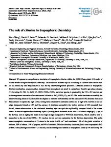
5. Nitrate Partition [36] Tang et al. [2004] discussed nitrate partitioning between the gas and aerosol phases for the ACE-Asia and TRACE-P experiments, and found that the regional model without aerosol considerations tended to overestimate nitrate acid (HNO3). Similar results [Neuman et al., 2003] were found for the ITCT 2K2 flights along the coast where regional pollutants interacted with sea salt, resulting in some of the nitric acid partitioning into the sea-salt particles. Figure 9 shows the simulated HNO3 mixing ratios with and without aerosol uptake compared to the measurements for WP-3 flights 4, 5, 8, and 9. The simulation with aerosol uptake had lower HNO3 concentrations than the simulation without aerosol for most segments of these flights. Because of the relatively coarse horizontal resolution, the simulation with aerosol underestimated most of the HNO3 peak values. The most significant differences between these two simulations appear for the predictions for background HNO3 levels. The simulation without aerosol uptake systematically overestimated the low background concentrations, especially for WP-3 flight 5, and it overestimated the HNO3 peak value for WP-3 flight 4. Under cation-limited conditions, the simulation with aerosol uptake can yield higher HNO3 values (Figure 9b) because of competition effects involving sulfates.

13 of 25

D23S11


Figure 7. (a – k) Simulated results at 2100 GMT, 15 May 2002. CO Asian ratios are presented with contour lines in Figures 7a and 7b. See color version of this figure at back of this issue. 14 of 25

D23S11

D23S11


D23S11

Figure 8. (a – g) STEM simulations compared to measurements for the WP-3 flight on 15 May.

However, over most clear oceanic sites, aerosol uptake tended to reduce gas-phase HNO3. This partitioning is an important factor causing the very low NOy ratio in the longdistance-transported Asian air masses (Figures 2a and 2b).

6. Nested Simulation for the Los Angeles Plume [37] WP-3 flight 10 performed an urban plume study over Los Angeles (LA) and surrounding areas. For this flight the contribution of Asian sources were small. The primary

domain over the eastern Pacific (Figure 1) with its 60-km horizontal resolution was not able to capture the fine structures caused by local emissions. Tang [2002] tested the multiscale simulation using nested domains in Nashville, Tennessee, and found that nesting predictions could better reflect power plant and urban plume structures. When the tenth WP-3 flight flew over LA and its downwind areas it encountered strong local plumes with steep concentration gradients, implying that local emissions played the dominant role on species concentrations. To simulate this sce-

15 of 25

D23S11


D23S11

Figure 9. (a – e) STEM simulations with and without the aerosol consideration compared to observations of four WP-3 flights, whose paths are shown in Figure 9e. See color version of this figure at back of this issue. nario, a domain with a 12-km horizontal nested grid within the primary eastern Pacific domain (Figure 1) was used. Simulated CO and O3 concentrations in the coarse and fine domains are shown in Figure 10. The coarse and fine simulations produced qualitatively similar CO and O3 distributions, but the higher resolution highlights the fine-scale structures. During this flight a front passed over LA region. Figure 10a shows that the low-altitude winds came from the northwest and turned southwesterly after passing over LA. In the upwind areas, west of longitude 119W, the coarse and nesting simulations did not show significant differences

for O3 and CO. Over and downwind of LA the nesting simulated CO showed two high zones (Figure 10a), while the coarse simulation had only one broad high-CO region (Figure 10b). The CO distributions mainly reflect the local emissions and transport effects. The elevated O3 regions in the nested-grid simulated did not overlap with the peak values of CO (as was the case for the coarse simulation), but instead were shifted downwind. The region of high ozone (>120 ppbv) was significantly smaller on the fine grid, indicating the effect of model resolution on photochemical processes.

16 of 25

D23S11


D23S11

Figure 10. (a– d) Nested (12-km resolution) and coarse (60-km resolution) simulated CO and O3 at 400 m at 2100 GMT, 13 May, for WP-3 flight 10 over Los Angeles and the surrounding area. See color version of this figure at back of this issue.

[38] To highlight the differences between these two simulations, the flight segment shown in Figure 10c, where the WP-3 aircraft operated around in and around LA, was analyzed further. Figure 11 shows these two simulations compared to the aircraft measurements. The simulated ethyne and propane concentrations using the nested grid were in much better agreement with the observations (Figures 11a and 11b). This is mainly due to the better resolution of the emissions, which enables a better representation of peak values. The refined high-resolution emissions better resolve the differences among urban, suburban and rural areas. [39] The lifetime of CO is much longer than ethyne or propane, and it also has a higher background concentrations and stronger emissions. Thus CO concentrations reflect the impacts of both local emissions and transport. Both the coarse and fine grid simulated CO capture the main altitude variations (Figure 11c), but the nested grid better represents the CO fine structures. Figure 11c also shows the simulated CO chemical net budgets, which vary in a manner consistent with that for the CO concentrations. The CO chemical budget is determined by the oxidations of CO and hydrocarbons. In the low-altitude areas around LA, hydrocarbons were elevated and CO had a positive net chemical budget that was positively correlated with the hydrocarbon concentrations. Most primary hydrocarbons tend to be coemitted with CO in this region, and thus high CO concentrations usually correspond to high hydrocarbon concentrations

(Figures 11a, 11b, and 11c). This is the reason why the CO net budget was correlated with CO concentration. For this flight the CO positive chemical budget helped to maintain the high CO concentration, but the high CO was mainly caused by strong emissions. The contribution of the CO chemical budget to CO concentrations was relatively weak, less than 2.5 ppbv/h (Figure 11c). [40] Both the fine and coarse grid simulations tended to overestimate O3 concentration, but the nested one shows better agreement with the observations (Figure 11d). The net O3 chemical budget for most of the flight segments was positive, up to 25 ppbv/h. For the flight segment after 2140 GMT the O3 concentrations followed the variations in the O3 chemical net budgets, implying that O3 production was the dominant influencing factor for O3 concentrations (as expected). The O3 chemical budgets on the fine grid show larger absolute values and variation than for the coarse grid, consistent with the better ability to resolve plume-like structures using the finer grid. The 12-km simulation improved the O3 prediction, but even finer grids are needed. [41] The improvement in ozone prediction with finer grids can be explained by looking at the predicted and observed NOz (NOy-NOx) concentrations (Figure 11e). As the photochemical product of NOx, NOz is usually highly correlated with O3 [Trainer et al., 1993]. The fine grid simulation shows a much better agreement with the observations, and the coarse grid tends to overestimate NOz. Figure 11e also shows the O3/NOz ratios. Both simulations

17 of 25

D23S11


D23S11

Figure 11. (a –h) Simulations compared to the measurements along the path of WP-3 flight 10 shown in Figure 10c. The nested and coarse simulations have similar J value predictions. So Figures 11g and 11h show only one simulation. See color version of this figure at back of this issue.

agree well with the observations for the flight segment before 2200 GMT, but tend to underestimate this ratio (especially for the coarse simulation) by overestimating NOz between 2200 GMT and 2300 GMT. The OPE difference between these two simulations and the observations

reflect their different photochemical behaviors, which is also highlighted by their OH differences (Figure 11f ). Both simulations systematically overestimated OH, but the nested simulation showed improvement for some flight segments (e.g., 2230 – 2330 GMT). However, the OH overestimation

18 of 25

D23S11


D23S11

Table 3. Observed and Simulated (60-km Resolution) Mean Values and Their Correlation Coefficients R for ITCT 2K2: All WP-3 Flights Below 1 km

1 km to 3 km

Above 3 km

Species and Variables

Observed

Modeled

R

Observed

Modeled

R

Observed

Modeled

R

Pressure, hPa Wind speed, m/s Relative humidity, % CO, ppbv O3, ppbv Ethane, ppbv Propane, ppbv Ethyne, ppbv SO2, ppbv Acetone, ppbv PAN, ppbv NO2, ppbv NO, ppbv HNO3, ppbv NOy, ppbv NOz, ppbv Toluene,a ppbv Xylene,a ppbv J[NO2], 1/s J[O3 ! O2 + O1D], 1/s J[H2O2], 1/s J[HNO3], 1/s J[HNO2 ! OH + NO], 1/s J[HCHO ! H + HCO], 1/s J[HCHO ! H2 + CO], 1/s

971.5 8.2 68.8 154 47.2 1.62 0.60 0.33 0.76 1.03 0.16 1.76 0.52 0.80 3.3 1.64 0.113 0.150 6.66 103 2.00 105 4.31 106 3.67 107 1.46 103 1.87 105 3.13 105

963.1 8.4 58.3 163 58.1 1.52 0.36 0.34 0.23 0.71 0.57 1.04 0.31 0.65 3.8 2.46 0.102 0.051 7.62 103 2.30 105 5.75 106 4.94 107 1.49 103 2.49 105 3.58 105

0.96 0.67 0.82 0.92 0.81 0.82 0.83 0.86 0.52 0.89 0.68 0.88 0.83 0.87 0.92 0.95 0.91 0.85 0.67 0.86 0.79 0.84 0.68 0.81 0.74

801.2 8.0 28.8 135 57.3 1.31 0.32 0.23 0.44 1.20 0.44 0.58 0.15 0.81 1.75 1.25 0.0492 0.0279 9.1 103 2.92 105 6.21 106 5.34 107 2.02 103 2.75 105 4.65 105

798.5 7.3 33.9 147 57.8 1.15 0.22 0.23 0.35 0.55 0.47 0.49 0.13 0.64 2.54 1.92 0.0604 0.0195 8.83 103 2.77 105 6.88 106 5.93 107 1.73 103 3.05 105 4.33 105

0.99 0.68 0.85 0.60 0.66 0.22 0.34 0.47 0.41 0.64 0.06 0.65 0.69 0.73 0.66 0.66 0.69 0.73 0.58 0.84 0.74 0.81 0.60 0.77 0.69

554.4 12.7 27.5 120 59.8 0.98 0.13 0.16 0.30 0.89 0.14 0.055 0.019 0.13 0.42 0.38 0.019 0.0047 0.010 2.95 105 6.72 106 5.47 107 2.26 103 3.20 105 5.58 105

551.7 11.5 28.2 113 64.0 0.77 0.06 0.11 0.10 0.27 0.15 0.018 0.009 0.12 0.42 0.40 0.017 0.0035 0.0092 2.77 105 7.10 106 5.90 107 1.81 103 3.37 105 4.70 105

0.99 0.88 0.73 0.18 0.47 0.40 0.30 0.14 0.18 0.28 0.26 0.43 0.43 0.60 0.51 0.57 0.18 0.20 0.56 0.83 0.77 0.83 0.59 0.79 0.69

a

Measured with proton-transfer-reaction mass spectrometry (PTR-MS).

is not caused by overprediction of the J values. Figures 11g and 11h show J [O3 ! O2 + O1D] and J[NO2] simulations compared to the observations. J[O3 ! O2 + O1D] is a key factor for clear-background OH, since O1D + H2O ! 2OH (reaction (R19) in Table 2) is the primary natural source of OH. The simulation agrees well with the observations for J[O3 ! O2 + O1D], but overestimates J[NO2]. However, the J[NO2] overestimation is much smaller than the OH or O 3 overestimations for the flight segments before 2300 GMT, indicating that OH overestimation may be associated with other process. The observed peak of OH appeared downwind of LA at low altitude (2300 GMT in Figure 11f ) where the observed J values were very low (Figures 11g and 11h). This implies that other photochemical processes had stronger influence on OH than the reaction (R19) only in the polluted area, which was also discussed before (Figure 6). Tang [2002] showed that nested simulation could have different photochemical relationship from the corresponding coarse simulation. In this WP-3 flight segment, these two simulations showed different responses to the same J values, because of their different pollutant loadings. Figure 11 shows that the nested simulation yielded better agreement with the observation than the coarse one for most flight segments, implying the impacts of changing resolution on emitted species, secondary generated species, and the photochemical system.

7. Mission-Wide Summary [42] The aircraft observations provide a valuable data set upon which to evaluate the models capabilities to simulate trace species distributions in the eastern Pacific. A missionwide summary of the model predicted and observed values are shown in Table 3. Presented are mean values for all

3-min-averaged observations and simulated values for the 13 WP-3 flights parsed into and averaged over three altitude layers. Also shown are the correlation coefficients R. The RAMS model driven by NCEP reanalysis data accurately represented the meteorological variables as shown for pressure, wind speed and relative humidity. In terms of trace gas species the highest mean concentrations are generally found below 1 km, indicative of the fact that low-altitude flights tended to sample air dominated by emissions from North America. PAN, HNO3, and acetone showed highest concentrations in the 1 –3-km layer, and O3 (peak value >3 km) are the exceptions. The model performed best in the lower altitudes, and for primary emitted species such as CO, ethane, propane, NO2, NO, and toluene. All species with the exception of SO2 and xylene are predicted within a factor of 2, and many within a factor of 1.2. The correlation coefficients for all the listed species are greater than 0.67. The predictions for the 1 – 3-km region for SO2, O3, NOz are usually better than the 3 km are markedly poorer, with R values typically lower than 0.5. J values are a notable exception, and are predicted with appreciable skill at all altitudes. J value predictions mainly reflected the simulations for aerosol optical properties and clouds. J[NO2] is very sensitive to fractional cloud, and the correlation coefficients for it are relatively low compared to predictions for other J values. [43] The values presented in Table 3 are a mixture of North-American- and Asian-emission-influenced air masses. To further evaluate the model performance, the data were stratified using model-calculated Asian ratios. The statistics for data points with Asian ratios 160 ppbv found at all altitudes. The highest values, however, were found below 2 km around LA. The model shows the same basic behavior and is able to accurately capture the mean behavior (as shown in Table 3 where the model mean values are within 6% of the observations at all altitudes). The distribution of the bias (simulated-observed) is presented in Figure 12c. The estimated VOC age is shown in Figure 12d, and reveals that aged air is found at all attitudes and latitudes. No simple relationship appears

Table 5. Observed and Simulated (60-km Resolution) Mean Values and Their Correlation Coefficients R for ITCT 2K2: WP-3 Flights With CO Asian Ratio >80% Below 1 km

1 km to 3 km

Above 3 km

Species and Variables

Observed

Modeled

R

Observed

Modeled

R

Observed

Modeled

R

CO, ppbv O3, ppbv Ethane, ppbv Propane, ppbv Ethyne, ppbv SO2, ppbv Acetone, ppbv PAN, ppbv NO2, ppbv NO, ppbv HNO3, ppbv NOy, ppbv NOz, ppbv J[NO2], 1/s J[O3 ! O2 + O1D], 1/s J[H2O2], 1/s J[HNO3], 1/s J[HNO2 ! OH + NO], 1/s J[HCHO ! H + HCO], 1/s J[HCHO ! H2 + CO], 1/s

129 40.7 1.29 0.20 0.20 0.21 0.48 0.060 0.25 0.074 0.077 0.40 0.23 7.53 103 1.89 105 4.63 106 3.70 107 1.65 103 2.00 105 3.45 105

121 38.1 0.97 0.11 0.23 0.021 0.43 0.075 0.020 0.008 0.058 0.24 0.21 9.23 103 3.02 105 7.13 106 6.26 107 1.80 103 3.16 105 4.45 105

0.90 0.74 0.95 0.97 0.85 0.02 0.77 0.77 0.12 0.28 0.35 0.30 0.007 0.31 0.72 0.54 0.66 0.34 0.59 0.47

127 53.2 1.23 0.18 0.19 0.21 0.86 0.089 0.035 0.011 0.070 0.30 0.26 9.88 103 3.23 105 6.82 106 5.87 107 2.20 103 3.07 105 5.12 105

118 47.5 0.86 0.08 0.17 0.09 0.35 0.094 0.011 0.006 0.053 0.23 0.22 1.03 102 3.59 105 8.30 106 7.33 107 2.02 103 3.78 105 5.21 105

0.46 0.31 0.73 0.87 0.64 0.35 0.18 0.76 0.01 0.19 0.28 0.38 0.53 0.61 0.81 0.75 0.80 0.62 0.76 0.70

125 64.4 1.03 0.13 0.17 0.32 0.92 0.15 0.026 0.008 0.058 0.34 0.34 0.0101 2.88 105 6.70 106 5.40 107 2.25 103 3.20 105 5.60 105

112 66.9 0.77 0.06 0.11 0.11 0.25 0.14 0.006 0.005 0.069 0.29 0.28 0.0104 3.34 105 8.22 106 6.94 107 2.06 103 3.94 105 5.42 105

0.085 0.46 0.44 0.33 0.17 0.26 0.18 0.33 0.30 0.18 0.25 0.31 0.31 0.63 0.83 0.83 0.85 0.66 0.84 0.76

20 of 25

D23S11


D23S11

Figure 12. Latitude-altitude distributions of (a and b) CO, (c) CO difference, (d) VOC age, (e) NOy, and (f ) NOy difference for all WP-3 flights. See color version of this figure at back of this issue.

between CO bias and air mass age. Similar results are found for observed and modeled NOy.

8. Trinidad Head Surface Site [45] During the ITCT 2K2 experiment extensive measurements were also performed at the Trinidad Head ground station (41.05N, 124.15W) located on the coast of northern California (Figure 1). The regional model was also used to provide forecast support and postanalysis interpretation to the surface observations. Figure 13 shows

the model simulations compared to the surface measurements from Julian day 110 to 143 (10 April to 13 May). Figure 13a shows that simulated wind speeds agreed with the observed diurnal peak wind velocities, and reflected their daily variation trend. However, because of the relatively coarse resolution the RAMS prediction failed to represent the nighttime calm winds at Trinidad Head. Both the RAMS prediction and the observations showed that north and northeast winds prevailed (Figure 13b). The simulated CO and NOy concentrations are consistent with the observation as shown in Figures 13c and 13d. Both the

21 of 25

D23S11


D23S11

Figure 13. (a – h) Simulation compared to surface observations at Trinidad Head. See color version of this figure at back of this issue.

observed and the simulated values show that CO and NOy are generally correlated. These two plots also show the CFORS simulated anthropogenic CO Asian ratio and NOx age. In general CO Asian ratios >0.5 are associated with air masses older than 50 hours. The highest NOy values occurred for air masses older than 50 hours. For example the CO and NOy peak concentrations on Julian days 113, 119– 120, and 132 were associated with low surface wind speeds, implying that these peaks were mainly due to the

accumulation of pollutants emitted from surrounding sources and transported to Trinidad Head under the low-windspeed situations. [46] Further insights into the role of local emission sources on Trinidad head is found in Figure 13e, where the simulated and observed propane, CFORS simulated VOC age, and observed methyl-t-butyl ether (MTBE), a compound mainly used in North America, are plotted. As shown the simulation results accurately capture the ob-

22 of 25

D23S11


served propane features. MTBE is a good tracer for local sources, as shown by its plume-like structure [Goldstein et al., 2004; Millet et al., 2004]. The MTBE peaks correlate with peaks in propane (and other pollutants), but propane shows broader maxima, reflecting the longer lifetime of propane. The simulated VOC age shows clearly a reversed variation with observed MTBE, providing further evidence for the utility of the VOC age indicator in helping to identify local and distant sources. As shown by the CO results in Figure 13c, the fresh pollution events at Trinidad Head are superimposed on air that is a mixture of Asian and American sources. [47] Both observed and simulated CO and propane show a clear declining trend during this one-month period (Figures 13c and 13e). The CO background concentration declined from 150 ppbv in April to 125 ppbv in May, while the propane background concentration declined from 0.3 to 0.15 ppbv. This seasonal variation trend reflects the increased CO and VOC consumptions by OH as the sunshine time became longer and photochemical reactions became more active (simulated daytime OH increased by about 30% during this period). [48] There were two instruments measuring aerosol ions at Trinidad Head: particle-into-liquid sampler (PILS) and the aerodyne Aerosol Mass Spectrometer (AMS) [Allan et al., 2004]. Both of these instruments report a cutoff diameter of 1 mm to capture submicron ions. The measured and simulated aerosol sulfate, nitrate and ammonium concentrations are presented in Figures 13f, 13g, and 13h, respectively. As discussed by Allan et al. [2004], the AMS instrument observed consistently more nitrate than the PILS instrument. This may be due to the presence of organic nitrates and/or amines. The simulated nitrate values are shown in Figure 13g for