30
African Journal of Information and Communication Technology, Vol. 5, No. 1, March 2009
Narrowband Interference Suppression in Wireless OFDM Systems Zlatka Nikolova1, Georgi Iliev 2, Miglen Ovtcharov3, and Vladimir Poulkov 4 Department of Telecommunications, Technical University of Sofia, Sofia, Bulgaria, e-mail: 1
[email protected]; 2
[email protected] ; 3
[email protected]; 4
[email protected] 1
Abstract—Signal distortions in communication systems occur between the transmitter and the receiver; these distortions normally cause bit errors at the receiver. In addition interference by other signals may add to the deterioration in performance of the communication link. In order to achieve reliable communication, the effects of the communication channel distortion and interfering signals must be reduced using different techniques. The aim of this paper is to introduce the fundamentals of Orthogonal Frequency Division Multiplexing (OFDM) and Orthogonal Frequency Division Multiple Access (OFDMA), to review and examine the effects of interference in a digital data communication link and to explore methods for mitigating or compensating for these effects. Index Terms—Adaptive complex systems, Adaptive signal processing, NBI suppression, OFDM, Wireless systems.
I. INTRODUCTION Orthogonal Frequency Division Multiplexing (OFDM) is a technology preferred for many telecommunication applications, such as broadband wireless communication systems [1]-[3]. These systems have relatively low transmission power, which makes them very sensitive to Narrowband Interference (NBI). The topic of NBI suppression, cancellation or avoidance for OFDM systems has been studied extensively in the last years and a variety of general approaches have been proposed. Because of the spectral leakage effect caused by Discrete Fourier Transform (DFT) demodulation at the OFDM receiver, many subcarriers near the interference frequency suffer serious Signal-to-Interference Noise Ratio (SINR) degradation, which could significantly degrade communications. Hence, NBI suppression is of primary importance for high speed broadband wireless communication systems. A brief overview of OFDM and Orthogonal Frequency Division Multiple Access (OFDMA) principles is presented in this paper. Special attention is given to several frequently-used NBI suppression methods. Experimental results for NBI suppression in Additive White Gaussian Noise (AWGN), Rayleigh, and Rician Manuscript received April 21, 2009. This work was supported by the Bulgarian National Science Fund – Grant No. ДО-02-135/2008 „Research on Cross Layer Optimization of Telecommunication Resource Allocation”.
channels are presented, illustrating the benefits of thecombined application. II. OFDM PRINCIPLES A. Basics of OFDM OFDM is quite similar to the well-known and oftenused technique of Frequency Division Multiplexing (FDM) [1]. OFDM uses the principles of FDM to allow several users to send messages over a single radio link. However, OFDM differs from FDM in a number of ways. In conventional broadcasting, each radio station transmits at a different frequency, using FDM to maintain the separation of the stations; there is no coordination or synchronization between these stations. Within an OFDM transmission, the information signals from numerous stations are combined into a single multiplexed stream of data. Afterwards, this data is transmitted using an OFDM ensemble made up of a dense packing of many subcarriers. All the subcarriers within the OFDM signal are time- and frequency-synchronized with each other, thus permitting the interference between subcarriers to be carefully controlled. The multiple subcarriers overlap in the frequency domain but do not cause Inter-Carrier Interference (ICI), due to the orthogonal nature of the modulation. As a rule, to prevent interference when using FDM, the transmitted signals need a frequency guardband between channels, which results in a lowering of the overall spectral efficiency. In contrast, OFDM allows a narrower-frequency guard-band, thus improving the spectral efficiency. OFDM achieves orthogonality in the frequency domain by mapping each of the separate information signals onto different subcarriers. The baseband frequency of a subcarrier is chosen to be an integer multiple of the fundamental frequency of the OFDM symbol. As a result, all subcarriers have a whole number of cycles per symbol and are orthogonal to each other. Fig. 1 shows the construction of an OFDM signal with four subcarriers. Their time waveforms are depicted in 1b, 2b, 3b, and 4b, whereas 1a, 2a, 3a, and 4a show the Fast Fourier Transform (FFT) responses. Individual subcarriers have 1, 2, 3, and 4 cycles per symbol and zero phases. The result of the summation of all four of the subcarriers is illustrated in 5a and 5b (Fig. 1).
1449-2679/$00 - (C) 2009 AJICT. All rights reserved.
31
African Journal of Information and Communication Technology, Vol. 5, No. 1, March 2009
1
20
(1a) 0
(1b) 10
-1
0
10
20
0
30
1
20
(2a) 0
(2b) 10
-1 1
0
10
20
(3a) 0 -1 1
20
0
10
20
0
30
20
10
15
0
5
10
15
0
5
10
15
0
5
10
15
0
5
10
15
(a)
(4b) 10 0
10
20
0
30
5
20
(5a) 0
(5b) 10
-5
5
(3b) 10
(4a) 0 -1
0
30
0
0
10
20
30
Time waveform (32 samples)
0
Carrier Frequency (using 32 point FFT)
Fig. 1. Time domain construction of an OFDM signal
A set of functions are reciprocally orthogonal if they meet the conditions in (1). If any two different functions within the set are multiplied, and integrated over a symbol period, the result is zero [2].
C , i = j i ≠ j.
∫ si (t )s j (t )dt = 0,
(1)
Equation (2) represents a set of orthogonal sinusoids, which correspond to the subcarriers for a non-modulated real OFDM signal. sin(2πkf a t ), for 0 < t < T , k = 1,2,...M sk (t ) = otherwise 0,
(2)
where fa is the carrier spacing, M is the number of carriers and T is the symbol period. Since the highest frequency component is Mfa, the transmission bandwidth is also Mfa. These subcarriers are orthogonal to each other, i.e. the result of the multiplication and integration of any two subcarriers waveforms over the symbol period is zero. Another approach to observing the OFDM signals’ orthogonality is via their spectra. In the frequency domain each OFDM subcarrier has a sin(x)/x frequency response, as shown in Fig. 2. The orthogonal nature of the transmission is due to the fact that each subcarrier peak coincides with the nulls of all other subcarriers. After a DFT is applied, a discrete spectrum is achieved and its samples are depicted in Fig. 2(a) by symbol ‘o’. When the DFT is time-synchronized, the frequency samples of the DFT correspond only to the peaks of the subcarriers. Thus, the overlapping frequency region between subcarriers does not affect the receiver. The measured peaks correspond to the nulls for all other subcarriers, thus providing the orthogonality of the subcarriers. Fig. 2(a) shows the spectra of the carriers and the discrete frequency samples seen by an OFDM receiver. The thick black line in Fig. 2(b) shows the overall combined response of all five subcarriers.
(b) Fig. 2. Subcarriers in a 5 tone OFDM signal - frequency response
B. OFDM Wireless Communication System As Fig. 3 indicates, an OFDM wireless communication system consists of three major parts: transmitter, channel, and receiver [2], [3], [8]. Transmitter - the transmitter takes the information data supplied by the information source, i.e. the information to be transmitted, and processes it in several steps to ensure reliable communication. If the source is analog, the information is first digitized by an Analog-to-Digital Converter (ADC). Generally the transmitter consists of a source encoder, a channel encoder, an interleaver, and a modulator. Source Encoder - the purpose of the source encoder is to remove as much redundancy as possible from the (digitized) output of the information source. Source encoding is also termed “data compression”. The sequence of binary digits from the source encoder is called the information sequence. Channel Encoder - The channel encoder introduces controlled redundancy into the binary information sequence by applying error-correcting codes. This redundancy is used by the channel decoder in the receiver to overcome the effects of noise and interference during the transmission of the signal through the channel. The two most important error-correcting coding techniques are block coding and convolutional coding. Interleaver - if errors occur in bursts, an effective method for improving error correction is to use interleaving. Interleaving is a controlled reordering of bits to avoid bit errors occurring in bursts at the decoder. By rearranging the coded data so that errors are separated by a large rather than a small number of bits, errors can be efficiently corrected using a random-error-correcting code. The two major interleaving techniques are blockinterleaving and convolutional-interleaving.
1449-2679/$00 - (C) 2009 AJICT. All rights reserved.
32
African Journal of Information and Communication Technology, Vol. 5, No. 1, March 2009
OFDM Digital Communication System SOURCE ENCODER
INFORMATION SOURCE
CHANNEL ENCODER
INTERLEAVER
DIGITAL MODULATOR
POWER AMPLIFIER
Transmitter WIRELESS CHANNEL
Receiver INFORMATION SINK
SOURCE DECODER
CHANNEL DECODER
DEINTERLEAVER
DIGITAL DEMODULATOR
INPUT STAGE
Fig. 3. Block diagram of a digital communication system (physical layer)
Digital Modulator - the primary purpose of the digital modulator is to map the binary information sequence into signal waveforms [4], [5]. If the information sequence is to be transmitted one bit at a time, the modulator may map each “0” into a waveform s0(t) and each “1” into a waveform s1(t). This is called binary modulation. Alternatively, the modulator may transmit l information bits at a time by using M=2l different waveforms si(t), i = 0, 1, …, M−1, one waveform for each of the 2l possible l-bit sequences. This is called M-ary modulation (M > 2), and the sequences of l bits are referred to as M symbols. A block diagram of an OFDM digital modulator is shown in Fig. 4. OFDM Digital Modulator
from Interleaver
OFDM MAPPING
IFFT
GUARD INTERVAL INSERTION AND WINDOWING
UP CONVERTER AND BPF
DAC AND LPF
to Power Amplifier
PILOT AND SYNCHRONIZATION INSERTION
Fig. 4. Block Diagram of a Digital Modulator
Guard Interval - the effect of Inter-Symbol Interference (ISI) on an OFDM signal can be improved by the addition of a guard interval to the start of each symbol. This guard interval is a cyclic copy that extends the length of the symbol. Fig. 5 shows the insertion of a guard interval. Copy IFFT
Guard Interval
IFFT output
TG Sumbol N-1
TFFT TS
Guard Interval
IFFT
Time Sumbol N+1
Sumbol N
Fig. 5. Addition of a guard interval to an OFDM signal
The total length of the symbol is: TS = TG + TFFT ,
(3)
where TS is the total length of the symbol in samples, TG is the length of the guard interval in samples, and TFFT is the size of the Inverse Fast Fourier Transform (IFFT) used to generate the OFDM signal. Power Amplifier - this is the output stage of an OFDM system. The Radio Frequency (RF) signal is amplified, shaped by the bandpass (BP) channel filter and supplied to the transmission antenna system. Two of the most crucial functions, determining the Quality of Service (QoS) of wireless systems are implemented here transmitted power control and antenna beam forming. Wireless Channel - the wireless channel introduces unintended distortion to the transmitted signal by, for example, adding noise and introducing fading, delayed reflections and interference [5]-[7]. Receiver - the task of the receiver is significantly more difficult than that of the transmitter. This is largely due to the need for synchronizing the timing, phase and frequency of the distorted received signal. Basically, a receiver consists of: input stage, demodulator, deinterleaver, channel decoder and source decoder. Input Stage - the input stage incorporates several functions, such as: receiving antenna gain control, adaptive notch filter for NBI suppression, low noise amplifier, channel estimation, and equalization and automatic gain control. Digital Demodulator - the digital demodulator is usually the most complex part of a communication system. Here, the timing, phase and frequency of the received signal is detected and then tracked to ensure synchronization [3], [4], [6], [7]. The demodulator processes the channel-corrupted transmitted waveform and converts each waveform to a single number that represents an estimate of the transmitted data symbol. The demodulator consists of several parts. Usually, the received signal is fed through a matched filter or, alternatively, a correlator. The output from the filter/correlator is sampled at symbol rate, and passed on to a detector, which makes a decision as to which symbol was transmitted. The detector can employ soft decision or hard decision detection. A block diagram of a demodulator is shown in Fig. 6.
1449-2679/$00 - (C) 2009 AJICT. All rights reserved.
33
African Journal of Information and Communication Technology, Vol. 5, No. 1, March 2009 OFDM Coherent Digital Demodulator
from AGC DOWN CONVERTER AND LPF
ADC
GUARD INTERVAL REMOVAL AND WINDOWING
FREQUENCY AND PHASE RECOVERY
FFT
TIME RECOVERY
CHANNEL CORRECTION
are the Rayleigh and Rician fading models. An example of time varying impulse response of a fading channel is given in Fig. 7.
OFDM DEMAPPING
to Deinterleaver
Fig. 6. Block Diagram of a Digital Coherent Demodulator
Deinterleaver - at the receiver, a deinterleaver is employed to undo the effect of the interleaver in the transmitter [1], [2]. In order to ensure proper deinterleaving, the interleaver and deinterleaver must be synchronized. In the case of block interleaving, this means that bits interleaved in the same frame must also be deinterleaved in the same frame. Convolutional interleavers and deinterleavers are finite state machines, and must be in the same initial state Channel Decoder - the channel decoder attempts to reconstruct the original information sequence from knowledge of the code used by the channel encoder and the redundancy in the received data [1], [2]. As with deinterleaving, decoding requires synchronization. The block decoder must know where in the received bit sequence a code word begins and the convolutional decoder must know what state to start in. Source Decoder - from the knowledge of the source encoding method used, the source decoder attempts to reconstruct the original signal of the source. The result, an estimation of the transmitted information, is then finally passed to the information sink C. Wireless Fading Channel Small-scale fading or simply “fading”, is a random variation of the received signal’s envelope, phase, and frequency. This fading is a result of the summing of signals from several paths (direct, reflected, scattered, etc.) at the receiver antenna [8], [9]. A wireless channel is a good example of a fading channel. The three most important fading effects caused by this multipath propagation are: rapid changes in signal strength over a small travel distance or time interval, random frequency modulation due to varying Doppler shifts in different multipath signals, and time dispersion (echoes) caused by multipath propagation delays. Examples of short term fading and frequency selective fading are shown in Fig. 7 and Fig. 8. To better characterize the fading signal, a number of statistical measures are used [4], [7]. The time and frequency dispersive properties of the channel are described by its root mean square (rms) delay spread and coherence bandwidth, and its coherence time and Doppler spread, respectively. Although analytical expressions do not exist for the general case, probability distributions that describe these variations are known for a few welldefined situations. Among these, the most frequently used
Fig. 7. Plot of Short-Term Fading with distance
Fig. 8. Plot of Frequency selective fading
Fading Channel Parameters - the time dispersive properties of the channel, i.e., its rms delay spread and coherence bandwidth, are derived from its power delay profile. The power delay profile defines the delays and relative powers of different multipath signals, and is heavily dependent on the particular surroundings. The coherence bandwidth is a statistical measure of the range of frequencies over which the channel can be considered “flat”, i.e. a channel that passes all spectral components with approximately equal gain and linear phases. If the coherence bandwidth is defined over which the frequency correlation function is above 0.5 (which is sufficient for all practical purposes), the coherence bandwidth is approximately [8], [9]: 1 , 5σ τ
BC ≈
(4)
where στ is the rms delay spread defined as: σ τ = τ 2 − (τ) 2 ,
(5)
with τ=
∑ P(τ j )τ j j
∑ P(τ j )
, and τ 2 =
j
∑ P(τ j )τ j j
∑ P(τ j )
.
(6)
j
Here, P(τj) refers to the received signal power at delay τj from the first received signal component at τ0 =0.
1449-2679/$00 - (C) 2009 AJICT. All rights reserved.
34
African Journal of Information and Communication Technology, Vol. 5, No. 1, March 2009
The Doppler frequency spread BD is defined as the range of frequencies over which the received Doppler spectrum is approximately non-zero. When a pure sinusoidal tone of frequency fc is transmitted, the received signal spectrum, the Doppler spectrum, will have components in the range from fc – fd to fc + fd, where fd is the Doppler shift. The coherence time TC is a statistical measure of the time duration over which the channel impulse response is more or less invariant, and is inversely proportional to the Doppler spread BD: TC =
3 4 π BD
.
(7)
Fading Channel Types - depending on the relation between the signal parameters (such as bandwidth and symbol period) and the channel parameters (such as rms delay spread and Doppler spread), transmitted signals will undergo different types of fading. The multipath time delay spread determines whether the channel fading is flat or frequency-selective, whereas the Doppler spread determines whether it is fast or slow [6], [9]. The channel is classified as a flat-fading channel if the rms delay spread is smaller than the symbol period. The Rayleigh and Rician fading models both describe flatfading channels. If the rms delay spread is larger than the symbol period, the channel exhibits frequency selective fading. As a rule of thumb, the channel is considered frequency-selective if στ ≥ TS /10. Models for such channels are difficult to construct and are usually modeled as linear filters. In a fast fading channel, the Doppler spread is large and the coherence time is smaller than the symbol period. The channel variations are faster than those of the baseband signal, causing distortion at the receiver. If the Doppler spread is so small that the coherence time is much larger than the symbol period, the channel variations are slower than those of the baseband signal, and the channel is classified as a slow fading channel. In such a channel, the effects on signal amplitude and phase can be considered constant during one or several modulation symbol periods. Moreover, in a slow fading channel, the effects of Doppler spread are negligible at the receiver. The two most commonly-used models of fading channels are the Rayleigh and the Rician fading channel models. Both describe slow, flat-fading channels. Also they are often essential parts of models of frequencyselective channels. III. OFDM IMPLEMENTATION IN MULTIPLE ACCESS SCHEMES As well as a modulation scheme, OFDM could be used as part of a multiple access technique. “Multiple access” refers to the sharing of a communication resource by several users. Multiple access schemes attempt to distribute the resources in such a way as to provide orthogonal, i.e. non-interfering, communication channels for each user. The basic ways of distributing a communication resource are Frequency Division (FD),
Time Division (TD), and Code Division (CD). In Frequency Division Multiple Access (FDMA), each user receives a unique carrier frequency and bandwidth. In Time Division Multiple Access (TDMA), each user is given a unique time slot, either on demand or in fixed rotation. Orthogonal Code Division Multiple Access (CDMA) systems allow each user to share the bandwidth and time slots with many other users, relying on orthogonal binary codes to separate the users [10]-[12]. FDMA can be implemented in OFDM systems by assigning different users their own sets of subcarriers, as shown in Fig. 9. There are a number of ways this allocation can be performed. The simplest method is a fixed allocation of subcarriers to each user, as shown on the left of Fig. 9. An improvement of the fixed allocation scheme is dynamic subcarrier allocation based upon the channel state conditions. For example, due to frequency selective fading one user may have relatively good channels on some subcarriers, whereas another user might have good channels on other subcarriers. It could be mutually beneficial for these users to swap the fixed allocations given above, based on a dynamic allocation scheme. Besides FDMA, multiple users can also be accommodated with TDMA, where they are provided with a fixed or dynamic assignment in time. Fixed TDMA is shown on the right of Fig. 9. Such a TDMA scheme is appropriate for constant data-rate (i.e. circuit switched) applications like voice and streaming video. Dynamic assignment schemes (such as packet-based systems) employ more sophisticated scheduling algorithms based on queue-lengths, channel conditions, and delay constraints to achieve much better performance than fixed TDMA. In OFDM-TDMA, a particular user is given all the subcarriers of the system for any specific OFDM symbol duration. Thus, the users are separated via time slots. All symbols allocated to all users are combined to form an OFDM-TDMA frame. The number of OFDM symbols per frame can be varied based on each of the users’ requirements. Power
Time
Power
Time
User 3 User 2 User 1
User 1
Block of Subcarriers
User 2
User 6 User 5
User 4
User 9 User 8
User 7
User 3
Frequency
Block of Subcarriers
Frequency
Fig. 9. FDMA (left) and FDMA with TDMA (right)
In CDMA, each user is assigned a unique code sequence (spreading code) used to encode that user’s information-bearing signal; the users share time and frequency slots but employ different codes that allow the users to be separated by the receiver, as illustrated in Fig. 10. The receiver, knowing the code sequences of the user, decodes the received signal after reception and recovers
1449-2679/$00 - (C) 2009 AJICT. All rights reserved.
35
African Journal of Information and Communication Technology, Vol. 5, No. 1, March 2009
the original data. This is possible because the crosscorrelations between the code of the desired user and the codes of the other users are small. Because the bandwidth of the code signal is chosen to be much larger than that of the information bearing signal, the encoding process enlarges (spreads) the spectrum of the signal and is therefore also known as spread spectrum modulation. A channel in a CDMA system is then defined by the spreading code. Ideally, the codes among terminals should be orthogonal so that the receiver can detect the signal addressed to it in the presence of interference from other users. CDMA is the dominant multiple access technique for present cellular systems, but is not particularly appropriate for high-speed data since the entire premise of CDMA is that a bandwidth much larger than the data rate is used to suppress the interference. In wireless broadband networks the data rates already are very large, so spreading the spectrum further is not viable. OFDM and CDMA can be combined to create a MultiCarrier CDMA (MC-CDMA) waveform. It is possible to use spread spectrum signaling and to separate users by codes in OFDM by spreading in either the time or frequency domain. Time domain spreading entails each subcarrier transmitting the same data symbol on several consecutive OFDM symbols, that is, the data symbol is multiplied by a length N code sequence and then sent on a specific subcarrier for the next N OFDM symbols. Frequency domain spreading, which generally has slightly better performance than time domain spreading, entails each data symbol being sent simultaneously on N different subcarriers. In such a case the advantage is that OFDM provides a simple method to overcome the ISI effect of the multi-path frequency selective wireless channels, whereas CDMA provides the frequency diversity and the multi-user access scheme. MC-CDMA has gained much attention, because the signal can be easily transmitted and received using the FFT device without increasing the transmitter and receiver complexities and is potentially robust to channel frequency selectivity with good frequency use efficiency. Time
Power
User 1 User 2 User 3 User 4 User 5 Frequency
Fig. 10. User assignment in CDMA
OFDM could be used both as a modulation scheme and as part of the multiple access technique, by applying a spreading code in the frequency domain which as a result gives OFDMA. In OFDMA, the multiple access is realized by providing each user with a fraction of the available number of subcarriers. The available subcarriers are distributed among all the users for
transmission at any time instant. The subcarrier assignment is made for the user lifetime, or at least for a considerable time-frame. In this way, OFDMA could be considered as an ordinary FDMA; however, OFDMA avoids the relatively large guard-bands that are necessary in FDMA to separate different users. The scheme was first proposed for CATV systems and later adopted for wireless communication systems. OFDMA can support a number of identical downstreams, or different user data rates, e.g. assigning a different number of sub-carriers to each user. Based on the sub-channel condition, different baseband modulation schemes can be used for the individual sub-channels, for example Quadrature PhaseShift Keying (QPSK), 16-QAM, and 64-QAM etc. This is referred to as adaptive subcarrier, bit, and power allocation or QoS allocation. Very often a mixture of OFDMA and TDMA is applied, arranging the transmission in such a way that different users transmit in different time-slots, which may contain one or several OFDM symbols. Also frequency hopping (one form of spread spectrum realization) could be employed to provide security and resilience against inter-cell interference. A. Advantages of OFDMA OFDM and in particular, its IFFT/FFT implementation gave FDMA a new life as a broadband multiple access scheme. The use of IFFT/FFT allowed terminals to arbitrarily combine multiple frequencies (subcarriers) at baseband, leading to OFDMA. As stated above, OFDMA could be viewed as a hybrid of FDMA and TDMA; users are dynamically assigned subcarriers (FDMA) in different time slots (TDMA). The advantages of OFDMA start with the advantages of single user OFDM in terms of robust multipath suppression and frequency diversity. In addition, OFDMA is a flexible multiple access technique that can accommodate many users with widely-varying applications, data rates, and QoS requirements. Because the multiple access is performed in the digital domain (before the IFFT operation), dynamic and efficient bandwidth allocation is possible. This allows sophisticated time and frequency domain scheduling algorithms to be integrated in order to best serve the users. When comparing the three major types of systems for OFDM multiple access, i.e. OFDM-TDMA, OFDMCDMA (MC-CDMA or MC DS-CDMA), and OFDMA, it must be noted that OFDMA is fundamentally more advantageous than OFDM-TDMA and OFDM-CDMA when it comes to real system applications. The first major advantage is the better data rate granularity based on both time and frequency domain assignment. Early broadband systems utilized OFDMTDMA to offer a straightforward way of multiple accessing, where each user uses a small number of OFDM symbols in a time slot and multiple users share the radio channel through TDMA. The method has two obvious shortcomings: first, every time a user utilizes the channel, it has to burst its data over the entire bandwidth, leading
1449-2679/$00 - (C) 2009 AJICT. All rights reserved.
36
African Journal of Information and Communication Technology, Vol. 5, No. 1, March 2009
to a high peak power and therefore low RF efficiency; second, when the number of sharing users is large, the TDMA access delay can be excessive. OFDMA is a much more flexible and powerful way to achieve multiple access with an OFDM modem. In OFDMA, the multiple access is not only supported in the time domain, but also in the frequency domain, just like traditional FDMA but minus the guard-band overhead. As a result, an OFDMA system can support more users with much less delay. The finer data granularity in OFDMA is an advantage for multi-media applications with diverse QoS requirements. Another important advantage is the smaller link budget for low-rate users. Since a TDMA user must burst its data over the entire bandwidth during the allocated time slots, the instantaneous transmission power (dictated by the peak rate) is the same for all users, regardless of their actual data rates. This inevitably creates a link budget deficit that handicaps the low-rate users. Unlike TDMA, an OFDMA system can accommodate a low-rate user by allocating only a small portion of his band, proportional to the requested data rate. Concerning practical realization, an advantage of the OFDMA system is the receiver simplicity with multi-user interference-free detection. OFDMA has the merit of easy decoding at the receiver side, as it eliminates the intra-cell interference avoiding CDMA type of multi-user detection. This is not the case in MC-CDMA, even if the codes are designed to be orthogonal. The signals of different users can only be detected jointly, since the code orthogonality is destroyed by the frequency selective fading. In MCCDMA users’ channel characteristics and responses must be estimated using complex joint estimation algorithms, which is not the case with OFDMA. Furthermore, OFDMA is the least sensitive multiple access scheme to system imperfections. Due to these features, OFDMA has been adopted in several modern wireless systems, e.g. IEEE 802.16a-e and IEEE 802.20. A significant advantage of OFDMA relative to OFDM is its potential to reduce the transmit power and to also relax the Peak-to-Average Power Ratio (PAPR) problem. The PAPR problem is particularly acute in the uplink, where power efficiency and cost of the power amplifier are extremely sensitive issues. By splitting the entire bandwidth among many users in the cell, each user utilizes only a small subset of subcarriers. Therefore, each user transmits with a lower PAPR (PAPR increases with the number of subcarriers), and also with far lower total power than if it had to transmit over the entire bandwidth. Lower data rates and bursty data are handled much more efficiently in OFDMA than in single user OFDM, or with TDMA or CDMA, since rather than having to blast at high power over the entire bandwidth, OFDMA allows the same data rate to be sent over a longer period of time using the same total power [13], [14]. Another important advantage of OFDMA is in relation to the multiuser diversity capability. Multiuser diversity gain arises from the fact that in a wireless system with many users, the achievable data rate of a given resource unit varies from one user to another. Such fluctuations
allow the overall system performance to be maximized by allocating each radio resource unit to the user that can best exploit it. OFDMA allows different users to transmit over different portions of the traffic channel spectrum. Since different users perceive different channel qualities, a deep faded channel for one user may still be favorable to another. Therefore, through judicious channel allocation, the system can potentially outperform interference-averaging techniques by a factor of up to 3 in spectrum efficiency [15], [16]. One of the major problems associated with transmitting information from subscriber premises is the NBI. In OFDM-based systems, the effect can be loss of subcarriers and degraded BER performance. NBI affects OFDM-TDMA much more severely than OFDMA systems. As only one user occupies the whole bandwidth, if the particular user is subdued with high SINR, then the whole system collapses. A low interference level jams a few carriers in OFDMA and slightly reduces the system capacity, whereas an OFDM-TDMA system can still operate at its full capacity. However, as the interference level exceeds a certain threshold, OFDM-TDMA entirely breaks down but OFDMA only loses a small percentage of its total capacity. NBI affects certain sub-carriers and only the users who are allocated those sub-carriers are affected by increasing NBI [17]. IV. NBI SUPPRESSION METHODS In this section we will focus on an NBI which is an inband signal in an OFDM system. This type of signal interference can be found in the new unlicensed frequency bands, e.g., the Industrial Scientific Medical (ISM) band, coming from systems such as Bluetooth or microwave ovens which interfere with OFDM-based Wireless Local Area Networks (WLAN), like Hiperlan II. Other examples of NBI are strong Radio Frequency Interference (RFI) from short-wave radio, Citizens’ Band (CB) radio and amateur “ham” radio which interfere with Hybrid Fiber Coaxial (HFC) networks and Digital Subscriber Lines (DSL). Ineffective cable shielding of a network may also permit the ingress of interference from external electrical devices in the home, such as TVs and computers. Let’s consider a strong NBI signal which resides within the same frequency band as a wideband OFDM signal. In this case, severe Signal-to-Noise Ratio (SNR) degradation is likely to occur across all OFDM subcarriers due to spectral leakage of the NBI signal from block processing in the OFDM receiver. In Fig. 11, the magnitude-squared of the received signal samples |X[k]|2 is plotted. For flat-fading channels it is straightforward to ascertain the fact that the highest peak corresponds to the subcarrier affected by NBI, as shown in Fig. 11(a). Fig. 11(b) shows that, in frequency-selective channels, the OFDM signal presents a large dynamic range, and some signal peaks can have values close to the peak induced by NBI. This observation indicates that the detection of NBI becomes difficult in frequency-selective channels, especially if the Signal-to-Interference Ratio (SIR)
1449-2679/$00 - (C) 2009 AJICT. All rights reserved.
37
African Journal of Information and Communication Technology, Vol. 5, No. 1, March 2009
is high [18].
Each frequency bin is compared to the threshold and, if it exceeds the threshold, its value is held at the threshold. After applying the IFFT, the signal is much less contaminated with narrow band interferences. B. Frequency Identification and Cancellation Method The complex baseband signal at the input of the receiver can be expressed as [20]: r (t ) = st (t ) ∗ h (t ) + n(t ) + i(t ) ,
Fig. 11. The magnitude-squared of FFT bins: |X[k]|2
A. Frequency Excision Method In this approach, an FFT-based frequency domain excision method is used to remove NBI [19]. The DFT output of each block of NFFT samples, rm,n is given by: N FFT
rm,n = ∑ rm,k e − j 2 πkn / N , k = 1,....N FFT ,
(8)
FFT
k =1
where rm,n is the digital complex baseband signal at the demodulator output. In the frequency domain, the NBI manifests itself as a peak in the spectra. By comparing the magnitude of each frequency bin to a threshold, and limiting those bins within the threshold, interferences can be excised. The effectiveness of the FFT-based method depends on the selection of the threshold. The following method is used for the determination of the threshold. The mean value of the logarithm amplitude of the frequency bins and its variance are computed [19]: N FFT
10 log10 rm , n
n =1
N FFT
Tmean = ∑ Tvar =
1 N FFT
,
N ∑ 10 log10 rm , n n =1 FFT
(
(9) 2
) − N1
FFT
2 N ∑ 10 log10 rm , n . (10) n =1 FFT
(
)
The threshold is determined according to the mean value and variance and is given by [19]: 1/ 2 Texcision = Tmean − αTvar .
(11)
The scale factor α in the above equation is adjusted to maintain the threshold at some value of the noise floor.
(12)
where r(t) is the complex baseband signal at the input of the receiver, s(t) is the complex output signal of the transmitter, h(t) is the complex impulse response of the channel, n(t) is the complex AWGN, and i(t) is the complex single tone NBI. In order to approach the problem of the NBI identification, firstly the frequency position of the interference tone has to be estimated, via an FFT-based algorithm. After sampling the received signal r(t) to obtain r(k), the FFT must be applied to this sequence via a Goertzel algorithm or using a butterfly lattice. It is important to note that appropriate setting of the sampling time T is a fundamental step; therefore, to increase the frequency resolution, an 8 times oversampling in a frequency domain is proposed. Firstly, all power spectrum properties of all signals constituting r(t) are known. In fact, the power spectrum of an OFDM is strictly defined. Furthermore, the narrow band interfering signal can be modeled as a complex sinusoidal tone [20]: in (t ) = An e j ( ωnt +ϕn ) = an cos(ωn t ) + jbn sin(ωn t ) .
(13)
Secondly, it is clear that frequency domain processing is an appealing approach to estimating the frequency, because the spectral properties of r(t) are known. The frequency-cancelation method is implemented as a two-phase algorithm. At the beginning of the first phase, the complex NBI frequency is estimated by finding the maximum amplitude in the oversampled signal spectrum: ωn = arg ω ∈ L∞ max(PR (ω)) .
(14)
After that, the amplitude and phase estimation is done. The received sampled signal r(k) can be expressed as: r ( k ) = s ( k ) + n ( k ) + in ( k )
(15)
and the interference signal defined as: in (k ) = an cos(ωn k / T ) + jbn sin(ωn k / T ) .
(16)
A matrix form to represent the sampled interference can be used. Specifically, it can be rewritten in matrix form as: [ I ]n = [ M ].[ X ] .
(17)
The matrix [M] is defined as: cos(ωn k1 / T ) cos(ω k / T ) n 2 [M ] = ....... cos(ωn k N / T )
1449-2679/$00 - (C) 2009 AJICT. All rights reserved.
j sin(ωn k1 / T ) j sin(ωn k2 / T ) , ....... j sin(ωn k N / T )
(18)
38
African Journal of Information and Communication Technology, Vol. 5, No. 1, March 2009
and vector [X] gathers the coefficients an and bn:
[X ] =
an . bn
(19)
Applying the Maximum Likelihood (ML) algorithm, the solution is given by [22]:
[X ] = ([M ]T [M ]) [M ]T [R ] , −1
(20)
where the input signal vector [R] is defined as:
[R] = [r (k ) r (k ) 1
2
( )]
K rk
T
N
.
(21)
Thus the information about the complex amplitude of the NBI tone is derived. The second phase of the algorithm uses the estimation results from the first phase as the initial conditions of the Normalized Least Squares (NLS) optimization procedure [20]: N
M
i =1
m =1
f (ω, A, ϕ) = ∑ r (t ) − ∑ Am e
j (ω m t + ϕ m )
2
.
(22)
Here ωm is the frequency of the m-th interfering tone,
Αm and ϕm are the amplitude and phase respectively of the m-th interfering sinusoidal tone, and M is the total number of interfering tones. The sum from 1 to N is referred to the N samples representing the sampled monocycle. C. Nonlinear Filtering Methods Nonlinear ACM Filter for Autoregressive Interference The analysis begins by modeling the narrow band interference {ik} as a Gaussian autoregressive process of order p, i.e. assuming a model of the form [21], [22]: p
ik = ∑ φi i i =0
k
−i
+ ek ,
(23)
where {ek} is a white Gaussian process, and the autoregressive parameters Φ1, Φ2,…Φp are known to the receiver. Under this model, the received signal has a state space representation as follows [21]: xk = Φxk −1 + wk , z k = Hxk + sk + nk ,
[
the observation noise. Under this assumption, the filtered ) estimate and its conditional covariance Pk are xk obtained recursively through the update equations: Pk = M k − M k H T Gk ( z k ) HM k ,
(26)
) xk = x k + M k H T g k ( z k ) ,
(27)
M k +1 = Φ Pk ΦT + Qk , ) xk +1 = Φ xk ,
(28)
where ∂p( z k Z k −1 ) −1 . p z k Z k −1 , g k ( zk ) = − ∂z k ∂g k ( z k ) T , and Qk = E{wk wk }. Gk ( z k ) = ∂z k
[(
]
[
(30)
Adaptive Nonlinear Filter Based on an LMS Algorithm It has been shown in [24] that better interference rejection can be obtained by using a two-sided interpolation filter. For such a two-sided filter, shown in Fig. 12, the following Widrow Least Mean Squared (LMS) algorithm equations hold [22], [25]: X k = [z k + N , z k + N −1 , ... , z k +1 , z k −1 ,..., z k − N ] , T
(31)
θ k = [a− N (k ), a− N +1 (k ), ... , a−1 (k ), a1 (k ),..., a N (k )] , T
(32)
where 2N+1 is the length of the data window. zk
+
εk
pk(.)
+
zk
z-1 a1(k)
zk-1
z-1
zk-2
z-1
a2(k)
zk-L
aL(k)
(25)
]
+
T
where xk = ik ik−1 ... ik−p+1 , Hk=[1..0…0], wk = ek 0 ....0 , φ1 φ2 1 0 Φ= ... ... 0 0
)]
The ACM filter is thus seen to have a structure similar to that of the standard Kalman - Bucy filter. The timeupdate equations (27)-(28) are identical to those in the Kalman-Bucy filter. The measurement update of (30) involves correcting the predicted value by a nonlinear function of the prediction residual zk-Hxk. The nature of the nonlinearity is determined by the probability density of the observation noise.
(24) T
(29)
... φ p−1 φ p ... 0 0 . ... ... ... ... 1 0
zk
Fig. 12. Adaptive nonlinear filter based on LMS algorithm
The LMS algorithm can be normalized as follows [25]: µo 2 (33) ξ k X k , rk = rk −1 + µ o X k − rk −1 . rk The same approach as (23)-(30) is used to modify the adaptive linear prediction filter: θ k = θ k −1 +
The first component of the state vector xk is the interference ik. Hence, by estimating the state, an estimate of the interference which can be subtracted from the received signal to reject the interference, can be obtained. In [23], Masreliez has developed an Approximate Conditional Mean (ACM) filter for estimating the state of a linear system with Gaussian state noise and nonGaussian measurement noise. The nature of the nonlinearity is determined by the probability density of
L ) ) zk = ∑ ai (k − 1)[zk −i + ξ k −i ] . i =0
(34)
If the variance of the Gaussian random variable is σ 2k then the nonlinear transformation appearing in the ACM filter can be written as [25]:
1449-2679/$00 - (C) 2009 AJICT. All rights reserved.
39
African Journal of Information and Communication Technology, Vol. 5, No. 1, March 2009
ξ ρ k (ξ k ) = ξ k − tanh k2 . σk
(35)
By transforming the prediction error in (34) using the above nonlinearity, we get a nonlinear transversal filter for the prediction of zk [25]: L ) ) zk = ∑ ai (k − 1)[zk − i + ρk −1 (ξ k −1 ) ] .
performed at the input of the OFDM demodulator. In order to do this, a complex variable filter section with independent tuning of the central frequency and the bandwidth is used, which is then turned into adaptive to implement it in an OFDM receiver. A variable complex BP first-order realization named LS1 (Low Sensitivity) is used [28] – Fig. 13.
(36)
i =0
+
In order to implement the filter of (36), an estimate of the parameter σ 2k and an algorithm for updating the tap weights must be obtained.
∂zk . ∂θk −1
cos θ
+
Out Im
z-1 sin θ
sin θ
cos θ
+
In Im
z-1 + β
) where Yk = [z k −1 , z k −2 ,..., z k − L ]T and z k = zk + ρk (ξ k ) . Thus, the gradient algorithm (37) becomes, approximately [27]:
θ k = θ k −1 + µ Ψk ξ k ,
(39)
where: L
Ψk = Yk + ∑ ai (k − 1) xk − i Ψk − i
(40)
i =0
ξ ∂ρ k (ξ k ) 1 = 2 sec h 2 k2 ∂ξ k σk σk
+
+
In Re
(37)
For the nonlinear filter of (36), the LMS algorithm does not give a true gradient-based solution. Therefore, a modified gradient-based approach for (36) is considered [27]. Equation (36) can be rewritten as: ) z k = YkT θ k −1 , (38)
and xk = 1 −
Out Re
β
Nonlinear Gradient Algorithm Finding an adaptation strategy that minimizes the squared prediction error is the subject of interest in this section. A popular approach to this problem is to use a gradient descent solution [26], [27]:
θk = θk −1 + µ ξ k
+
.
(41)
From (40), it is seen that the vector Ψk is obtained by passing Yk through an L-th order IIR filter whose coefficients are the current estimates obtained by the gradient algorithm [27]: A(q -1 , k) = a1 (k )q -1 + a2 (k )q -2 + ... + aL (k )q -L .
(42)
At each stage, the stability of this polynomial must be checked and, if it is found to have any roots not within the unit circle, the parameter estimates must be projected onto that space where the polynomial is stable. D. Complex Adaptive Narrowband Filtering Compared with the desired wideband signal, the NBI occupies a much narrower frequency band, but with a higher power spectral density. On the other hand, the wideband signal usually has autocorrelation properties fairly similar to those of AWGN, so filtering in the frequency domain could be carried out. This filtering is
+
Fig. 13. Variable complex-coefficient first-order BP LS1 filter section
The transfer functions (all of them are of BP type) of the LS1 section are [28]:
H RR ( z)=H II ( z)=
[
]
βˆ 1 + 2βˆ cosθ z −1+ (2βˆ −1) z −2 , 1 + 2(2βˆ −1) cosθz −1+ (2βˆ −1)2 z −2
βˆ 2(1 − βˆ ) sinθz −1 , H RI ( z) = −H IR ( z) = 1+ 2(2βˆ −1) cosθz −1 + (2βˆ −1)2 z −2
(43)
where the composed multiplier βˆ is βˆ = β + 2β(β − 1) . The bandwidth can be tuned by trimming the single coefficient β, whereas θ controls the central frequency . This implementation has two very important advantages: firstly, an extremely low passband sensitivity increases the resistance to quantization effects; secondly, the central frequency and filter bandwidth can be independently controlled over a wide frequency range. In Fig. 14 the adaptive complex bandstop (BS)/BP narrowband system based on the LS1 variable complex filter section is shown. ADAPTIVE ALGORITHM
+
xR(n) xI(n)
eR(n) yR(n)
FIRST ORDER VARIABLE COMPLEX FILTER
yI(n) +
eI(n)
Fig. 14. Block-diagram of a BP/BS adaptive complex filter section
In the following we consider the input/output relations for corresponding BP/BS filte (44)-(50). For the BP filter we have the following real output:
1449-2679/$00 - (C) 2009 AJICT. All rights reserved.
40
African Journal of Information and Communication Technology, Vol. 5, No. 1, March 2009
y R (n) = y R1 (n) + y R 2 (n) ,
(44)
y R1 (n) = −2(2β − 1) cos θ(n) y R1 (n − 1) − − (2β − 1) y R1 (n − 2) + 2βx R (n) + 2
(45)
+ 4β cos θ(n) x R (n − 1) + 2β(2β − 1) x R (n − 2), y R 2 (n) = −2(2β − 1) cos θ(n) y R 2 (n − 1) −
(46)
− 4β(1 − β) sin θ(n) x I (n − 1),
where yR is the real output and xR is the real input. The imaginary output is given by the following equation: y I (n) = y I 1 (n) + y I 2 (n),
(47)
y I 1 (n) = −2(2β − 1) cos θ(n) y I 1 (n − 1) − − (2β − 1) 2 y I 1 (n − 2) +
(48)
+ 4β(1 − β) sin θ(n) x R (n − 1), and y I 2 (n) = −2(2β − 1) cos θ(n) y I 2 (n − 1) − − (2β − 1) 2 y I 2 (n − 2) + 2βx I (n) +
(49)
+ 4β cos θ(n) x I (n − 1) + 2β(2β − 1) x I (n − 2), 2
where yI is the imaginary output and xI is the imaginary input. For the BS filter we have real and imaginary outputs: e R ( n) = x R ( n) − y R ( n) , e I ( n ) = x I ( n ) − y I ( n ) .
(50)
The cost function is the power of the BS filter output signal: ∗
(51)
[e(n) e (n)],
where e(n) = eR (n) + jeI (n) . We apply the LMS algorithm to update the filter coefficient responsible for the central frequency as follows: ∗
θ(n + 1) = θ(n) + µ Re[e(n) y ' (n)] . (52) µ is the step size controlling the speed of convergence, (*) denotes complex-conjugate, y’(n) is the derivative of y(n)= yR(n)+j yI(n) with respect to the coefficient subject of adaptation. The real part of y’(n) is: y R' (n) = 2(2β − 1) sin θ(n) y R1 (n − 1) − − 4β 2 sin θ(n) x R (n − 1) + + 2(2β − 1) sin θ(n) y R 2 (n − 1) −
(53)
− 4β(1 − β) cos θ(n) x I (n − 1). ’
The imaginary part of y (n) is: y (n) = 2(2β − 1) sin θ(n) y I 1 (n − 1) + ' I
+ 4β(1 − β) cos θ(n) x R (n − 1) + + 2(2β − 1) sin θ(n) y I 2 (n − 1) −
K . (55) Lσ 2 In this case L is the filter order, σ2 is the power of the signal y’(n) and K is a constant depending on the statistical characteristics of the input signal. In most practical situations, K is approximately equal to 0.1 0 0, which is due to the amplitude and phase distortion of the filter. The degradation could be reduced by the implementation of a higher-order notch filter or avoided by simply switching off the filter, when SIR > 0.
1449-2679/$00 - (C) 2009 AJICT. All rights reserved.
42
African Journal of Information and Communication Technology, Vol. 5, No. 1, March 2009
Fig. 17. BER as a function of SIR for Rician channel of different NBI suppression approaches
VI. CONCLUSION
In this introductory paper, along with an overview of OFDM and OFDMA principles, particular attention is given to the basics of NBI mitigation techniques. The main idea behind this approach is to generalize the NBI suppression methods for Multiple Input Multiple Output (MIMO) OFDM wireless communication systems. The goal is to develop practical and effective solutions to deal with inter-cell interference problems for multi-cell MIMO systems, thus allowing for continuous improvement of the system throughput and QoS. REFERENCES [1] [2] [3] [4] [5] [6] [7] [8] [9] [10] [11] [12]
[13] [14] [15] [16] [17]
R. van Nee, R. Prasad, OFDM for Wireless Multimedia Communications, Artech House, 2000. H. Shulze, C. Luders, Theory and Applications of OFDM and CDMA, Wiley, 2005. H. Lui, G. Li, OFDM-Based Broadband Wireless Networks, Wiley, 2005. S. Sampei, Applications of Digital Wireless Technologies to Global Wireless Communications, Prentice Hall, 1997. M. Jeruchim, P. Balaban, and K. Shanmugan, Simulation of Communication Systems, Kluwer Academic, 2000. W. Jakes, Microwave Mobile Communications, IEEE Press, 1974. W. Lee, William, Mobile Communications Design Fundamentals, Wiley, 1993. W. Zou, Y. Wu, “COFDM: An Overview”, IEEE Transactions on Broadcasting, vol. 41, No 1, March 1995. M. Chryssomallis, “Simulation of mobile fading channels”, IEEE Antenna’s and Propagation Magazine, vol. 44, No 6, Dec. 2002. R. Prasad, OFDM for Wireless Communications Systems, Artech House, 2004. A. Goldsmith, Wireless Communications, Cambridge University Press, 2005. P. Jung, P. Baier, and A. Steil. “Advantages of CDMA and spread spectrum techniques over FDMA and TDMA in cellular mobile radio applications”, IEEE Trans. on Vehicular Technology, pp. 357–364, Aug. 1993. S. Hara and R. Prasad. “Overview of multicarrier CDMA”, IEEE Communications Magazine, vol. 35, pp. 126–33, Dec. 1997. X. Gui and T. S. Ng. “Performance of asynchronous orthogonal multicarrier system in a frequency selective fading channel”, IEEE Trans. on Communications, vol. 47, pp.1084–1091, July 1999. H.Liu and G. Li., OFDM – Based Broadband Wireless Networks. Design and Optimization, Wiley, 2005. WiMAX Forum website, MobileWiMAX – Part I: A Technical Overview and Performance Evaluation, Online: available http://www.wimaxforum.org. H. Sari et al., “An analysis of orthogonal frequency-division multiple access,” GLOBECOM, vol. 3, Nov. 1997, pp. 1635–1639.
[18] A. Giorgetti, M. Chiani, M. Win, “The effect of narrowband interference on wideband wireless communication systems”, IEEE Trans. Communications, vol. 53, No.12, pp.2139-2149, Dec. 2005. [19] Jyh-Ching Juang, Chung-Liang Chang, Yu-Lung Tsai, ”An interference mitigation approach against pseudolites”, 2004 Int. Symposium on GNSS/GPS, Sydney, Australia, 6 – 8 Dec. 2004. [20] E. Baccareli, M. Baggi, L. Tagilione, “A novel approach to inband interference mitigation in ultra wide band radio systems”, IEEE Conf. on Ultra Wide Band Systems and Technologies, 2002. [21] F. M. Hsu and A. A. Giordano, “Digital whitening techniques for improving spread-spectrum communications performance in the presence of narrow-band jamming and interference,” IEEE Trans. on Communications, vol. COM-26, pp. 209-216, Feb. 1978. [22] R. A. Iltis and L. B. Milstein, “An approximate statistical analysis of the Widrow LMS algorithm with application to narrow-band interference rejection,” IEEE Trans. on Communications, vol. COM-33, pp. 121-130, Feb. 1985. [23] C. J. Masreliez, “Approximate non-Gaussian filtering with linear state and observation relations,” IEEE Trans. Automatic Control, vol. AC-20, pp. 107-110, Feb. 1975. [24] S. Sampei, Applications of Digital Wireless Technologies to Global Wireless Communications, Prentice Hall, 1997. [25] C. R. Johnson, “Adaptive IIR filtering: current results and open issues,” IEEE Trans. on Information Theory, vol. IT-30, pp. 237250, Mar. 1984. [26] B. Friedlander, “System identification techniques for adaptive signal processing,” IEEE Trans. Acoustic, Speech, Signal Processing, vol. ASSP-30, pp. 240-246, Apr. 1982. [27] R. Vijayanan, H. Vincent Poor, “Nonlinear techniques for interference suppression in spread-spectrum systems”, IEEE Trans. on Communications, vol. 38, No. I, July 1990. [28] G. Iliev, Z. Nikolova, G. Stoyanov, K. Egiazarian, “Efficient design of adaptive complex narrowband IIR filters”, Proceedings of XII European Signal Processing Conference, EUSIPCO 2004, Vienna, Austria, pp. 1597 - 1600, 6 - 10 Sept. 2004. [29] S. Douglas, Adaptive filtering, in Digital Signal Processing Handbook, D. Williams and V. Madisetti, Eds., CRC Press, 1999. Zlatka Nikolova received her M.Eng. and Ph.D. degrees in Telecommunications at the Technical University of Sofia, Bulgaria, in 1988 and 2008, respectively. Her current position is Assistant Professor at the Department of Communication Networks, Faculty of Telecommunications, Technical University of Sofia, Bulgaria. Her main research interests include Communication Circuits, Digital Signal Processing, and Efficient Digital Filtering. Georgi Iliev received M.Eng. and Ph.D. degrees in Telecommunications from Technical University of Sofia, Bulgaria, in 1990 and 1996, respectively. Since 2003, he has been an Associate Professor in the Technical University - Sofia. His main research interests are in Digital Signal Processing, Communication Networks, and Adaptive Communication Systems. Miglen Ovtcharov received B.Eng. and M.Eng. degrees in Telecommunications from the Technical University of Sofia, Bulgaria, in 1989 and 1991, respectively. In 1994, he received a Postgraduate Specialist in Applied Mathematics and Computer Science degree from the Technical University of Sofia. Since 2005, he has been a Ph.D. student in Broadband Digital Communications at the Technical University of Sofia. His main research interests are in xDSL Technologies, Digital Wireless Communications and Digital Signal Processing. Vladimir Poulkov received M.Eng. and Ph.D. degrees in Telecommunications from the Technical University of Sofia, Bulgaria, in 1981 and 1995, respectively. Since 2000, he has been an Associate Professor at the Technical University of Sofia. Presently he is Dean of the Faculty of Telecommunications. His main research interests are in Digital Transmission Systems, Information Theory, Multiple-Access Control Methods.
1449-2679/$00 - (C) 2009 AJICT. All rights reserved.