energy system models are driven by 'useful demand', while national statistics ...... (1978) compare two different future Swedish scenarios, one with solar .... the system planner and of focusing on the real problem, e.g. 'kids are starving in great.
THESIS FOR THE DEGREE OF DOCTOR OF PHILOSOPHY
National Energy System Modelling for Supporting Energy and Climate Policy Decision-making: The Case of Sweden
ANNA KROOK RIEKKOLA
Department of Energy and Environment CHALMERS UNIVERSITY OF TECHNOLOGY Göteborg, Sweden 2015
National Energy System Modelling for Supporting Energy and Climate Policy Decision-making:
The Case of Sweden. ANNA KROOK RIEKKOLA ISBN 978-91-7597-202-2 © ANNA KROOK RIEKKOLA, 2015
Doktorsavhandling vid Chalmers tekniska högskola Ny serie nr 3883 ISSN 0346-718X Department of Energy and Environment Division of Energy Technology Chalmers University of Technology SE-412 96 Göteborg Sweden Telephone: +46 (0)31-772 10 00 http://www.chalmers.se/ee Printed by Reproservice, Chalmers University of Technology Göteborg, Sweden 2015
ii
To Mats, Nikolaj and Julia Finally, this book is to its end and I will be all yours
iii
iv
National Energy System Modelling for Supporting Energy and Climate Policy Decision-making: The Case of Sweden. ANNA KROOK RIEKKOLA Department of Energy and Environment, Division of Energy Technology Chalmers University of Technology, Göteborg, Sweden
ABSTRACT Energy system models can contribute in evaluating impacts of energy and climate policies. The process of working with energy system models assists the understanding of the quantitative relationships between different parts of the energy system and between different time periods, under various assumptions. With the aim of improving the ability of national energy system models to provide robust and transparent input to the decision-making process, a three-step energy modelling process is introduced based on the literature on system analysis and energy modelling. This process is then used to address five different research questions, which are based on (but not identical to) six embedded papers. In the first step (step 1) the ‘real’ system is simplified and conceptualised into a model, where the main components and parameters of a problem are represented. In order to attain robust results, it is important to focus not only on what needs to be included in the model, but also on what can be left out. In order not to add noise to the analysis, there is a trade-off between what is desired and what can be included in terms of data. In the second step (step 2), all assumptions are sorted within a mathematical model and the algorithms solved. The structure of the model is found crucial for the possibility to trace the results back to the assumptions (transparency). In the last step (step 3), the model results are interpreted together with aspects not captured in the model (e.g. non-economic preferences, institutional barriers), and discussed in relation to the direct assumptions provided to the model (step 1) and to the implicit assumptions due to the choice of model (step 2). All three steps are essential in order to achieve robust and transparent policy analyses, and all three steps contribute to the learning about the ‘real’ system. The embedded papers (Paper I-VI) deal with issues of particular relevance for long-term analysis of the Swedish energy system. The results of Paper I illustrate the importance of capturing the seasonal and daily variations when representing cross-border trade of electricity in national models; a too simplified representation will make the model overestimate the need for installed power capacity in Sweden. Paper II presents a methodology for estimating the ‘useful demand’ for heating and cooling based on national statistics, which is useful as most energy system models are driven by ‘useful demand’, while national statistics are based on the measurable ‘final energy consumption’. Paper III compares the technical potential of combined heat and power (CHP) from different approaches and calculates the economic potential of CHP using a European energy system model (EU-TIMES). The comparison the technical potential of the different approaches reveals differences in definitions of the potential as well as in the system boundary. The resulting economic potential of CHP in year 2030 is shown to be significantly higher compared to today’s level, even though conservative assumptions v
regarding district heating were used. Paper IV assesses the impacts of district heating on the future Swedish energy system, first by a quantitative analysis using TIMES-Sweden and then by discussing aspects that cannot be captured by the model. Paper V compares different climate target scenarios and examines the impacts on the resulting total system cost with and without the addition of ancillary benefits of reductions in domestic air-pollution. The results reflect the fact that carbon dioxide emission reductions abroad imply a lost opportunity of achieving substantial domestic welfare gains from the reductions of regional and local environmental pollutants. Paper VI presents and discusses an iteration procedure for softlinking a national energy system model (TIMES-Sweden) with a national CGE model (EMEC). Some aspects of the way in which we perform the soft-linking are not standard in the literature (e.g., the use of direction-specific connection points). By applying the iteration process, the resulting carbon emissions were found to be lower than when the models are used separately. Key words: TIMES-Sweden, energy system models, energy-economics, system analysis, cross-border trade, CHP, district heating, ancillary benefits, climate policy, soft-linking.
vi
LIST OF PUBLICATIONS
This thesis is based on the work contained in the six following papers. The papers will be referred to in the text by Roman numerals as follows. I.
Cross-Border Electricity Exchange and its influence on investment incentives in the Nordic Electricity Market. A. Krook Riekkola, E.O. Ahlgren and I. Nyström. Working paper based on a paper presented at the 26th IAEE International Conference, in 2003.
II.
Methodology to estimate the energy flows of the European Union heating and cooling market. N. Pardo, K. Vatopoulos, A. Krook-Riekkola, and A. Perez. Energy, Vol. 52 (2013), pp.339-352.
III.
Assessing the Development of Combined Heat and Power Generation in the EU. L. Stankeviciute and A. Krook Riekkola. International Journal of Energy Sector Management, Vol. 8 (2014), pp.76 – 99.
IV.
Long-term impacts of district heating – an explorative scenario study on Sweden. A. Krook Riekkola and L. Wårell. Working paper.
V.
Ancillary benefits of climate policy in a small open economy: The case of Sweden. A. Krook Riekkola, E.O. Ahlgren and P. Söderholm. Energy Policy, Vol. 39 (2011), pp. 4985-4998.
VI.
Challenges in Top-down and Bottom-up Soft-Linking: Lessons from Linking a Swedish Energy System Model with a CGE Model. A. Krook-Riekkola, C. Berg, E.O. Ahlgren and P. Söderholm. Based on a conference paper presented at the 32nd edition of the International Energy Workshop (IEW) in 2013. Submitted for potential publication.
Contribution by Anna Krook Riekkola to Papers I to VI: Krook Riekkola is the main author of Papers I and V and carried out data collection, modelling and analysis for these papers. Ahlgren and Nyström supervised Paper I and Ahlgren and Söderholm supervised Paper V, meaning they have contributed with ideas, discussions and editorial suggestions to these papers. In Paper II, Krook Riekkola was responsible for framing the study, for identification of the methodology (calculating the useful demand based on official statistical data) presented in Section 3, and for the first approach in the calculation and analysis of the energy flows presented in Section 4.
vii
In Paper III, Stankeviciute and Krook Riekkola made equal contributions as principal authors. Krook Riekkola was in particular responsible for the definition of the potential of combined heat and power (Section 2), the collection and analysis of new CHP data (Section 3.2) and the technology implication part of the analysis in Section 5. In Paper IV, Krook Riekkola was the main contributor of the methodology, choice of scenarios and the quantitative analysis with TIMES-Sweden (Section 3-5), while Krook Riekkola and Wårell made equal contributions to the qualitative analysis and the final conclusions (Section 6-7). In Paper VI, Krook Riekkola and Berg made equal contributions as principal authors. Krook Riekkola carried out the data analysis, modelling and analysis of the TIMES-Sweden model, while Berg made a similar contribution with respect to the EMEC model. The soft-linking was carried out as an integrated process between the two. Ahlgren and Söderholm contributed with ideas, discussions and editorial suggestions to the paper.
viii
Table of Contents Abstract ……………………………………………………….……………………………v List of Publications…………………………………………...……………………………vii Table of Contents…………………………………………………………………………..ix 1
Introduction .................................................................................................................. 1 1.1 Research context .......................................................................................................... 1 1.2 Aim, research questions and scope .............................................................................. 1 1.3 Central assumptions and delimitations ........................................................................ 3 1.4 Outline of this thesis .................................................................................................... 4
2
Methodology – Energy System Analysis..................................................................... 5 2.1 Systems theory ............................................................................................................. 5 2.2 The systems approach .................................................................................................. 8 2.3 Energy system analysis .............................................................................................. 10 2.3.1 2.3.2 2.3.3 2.3.4
Energy – from primary resource to end-use services ....................................... 11 Engineering – technology efficiency and system efficiency ............................ 11 Economics – the value of energy systems ........................................................ 12 Environment – pollution and other environmental impacts ............................. 12
2.4 Energy system models ............................................................................................... 14 2.5 Energy system modelling process.............................................................................. 16 3
Concepts Applied ....................................................................................................... 22 3.1 Potential ..................................................................................................................... 22 3.2 Scenarios .................................................................................................................... 23 3.3 Externalities ............................................................................................................... 24 3.4 Discounted total system cost...................................................................................... 24 3.5 Discount rate .............................................................................................................. 26
4
Characteristics of the Swedish Energy System.......................................................... 27 4.1 Historical development of the Nordic power market................................................. 27 4.2 Electricity generation mix .......................................................................................... 29 4.3 Electricity demand ..................................................................................................... 31 4.4 Swedish demand for space heating and warm water ................................................. 33 4.5 District heating ........................................................................................................... 35
5
TIMES-SWEDEN ..................................................................................................... 36 5.1 Model characteristics ................................................................................................. 36 5.2 Main assumptions ...................................................................................................... 39 5.3 Main data sources ...................................................................................................... 40
6
Reflections on uncertainties and validation ............................................................... 43 6.1 Energy balance (practical and external validation).................................................... 44 6.2 Consistency (internal validation) ............................................................................... 44 6.3 Level of details (practical validation) ........................................................................ 45 6.4 Reality check (external validation) ............................................................................ 45 6.5 Sensitivity analysis (internal validation).................................................................... 46 ix
6.6 Avoid black-box (theoretical validation) ................................................................... 47 6.7 Oversimplification (internal validation) .................................................................... 47 7
Challenges in National Energy System Modelling .................................................... 48 7.1 Cross-border trade...................................................................................................... 50 7.2 Combined heat and power in national energy system models ................................... 53 7.2.1 7.2.2 7.2.3 7.2.4
Defining CHP potentials .................................................................................. 54 Model representation to assess technical potential........................................... 56 Model representation to assess economic potential ......................................... 58 Estimation of technical and economic potential of CHP ................................. 61
7.3 District heating as part of the National Energy System ............................................. 61 7.4 Ancillary benefits from climate policy ...................................................................... 66 7.5 Linking CGE and energy system models .................................................................. 72 8
Main findings and contributions ................................................................................ 74 8.1 Cross-border trade...................................................................................................... 75 8.2 CHP in national energy systems models.................................................................... 76 8.3 District heating as part of the National Energy System ............................................. 77 8.4 Ancillary benefits from climate policy ...................................................................... 78 8.5 Linking CGE and energy system models .................................................................. 79
9
Conclusions, recommendations and further work ..................................................... 82 9.1 Conclusions and recommendations ........................................................................... 82 9.2 Further research ......................................................................................................... 84
Acknowledgement ............................................................................................................... 86 References…………………………………………………….……………………………88 Appended Papers I-VI
x
Introduction
1 Introduction This introductory section presents the research context followed by the aim of the research, the research questions and the scope. Finally, an outline of the thesis is presented.
1.1 Research context The balance of evidence suggests that anthropogenic emissions of greenhouse gases – of which carbon dioxide is the most significant – have a distinct negative impact on the global climate (e.g. IPCC, 2007). IPCC (2014a) stresses the importance of implementing strong and effective policy instruments. On 9 March 2007, the European Council adopted a new Energy Policy with binding targets for 2020 to reduce the climate impact of the energy system and facilitate sustainable, secure and competitive energy, or more exactly to i) reduce greenhouse gases by 20% from the 1990 level (EU level), ii) ensure 20% of renewables in the total energy mix (EU level), iii) plan to increase energy efficiency by 20% (EU level), and iv) ensure 10% of renewables in transportation fuels (national level) and a 2 degree vision for the year 2050 (EC, 2007). The Roadmap 2050 (EC, 2011) concludes that an 80% cut in CO2 emissions within the EU is needed in order to meet this 2 degree target. The advancement in science and technology helps in reaching these targets. Policy instruments can help immature technologies into the market. To identify which kind of actions to support, cost-effective pathways to reach the targets first need to be identified. Such pathways can, for example, be provided by energy system models, which can capture important interactions within the energy system and simulate competitive technology options in order to meet a given demand for goods and services under given constraints. Likewise, these models are able to analyse the effects of different policy instruments on the long-term development of the energy system. Pfenninger et al (2014) conclude in their review of energy models for twenty-first century energy challenges, that irrespectively of how energy systems modelling evolve, it is important that ‘the policy implications drawn are sound’. Thus, it is not only important to focus on the development on new models, but also to focus on what is inside the models and in understanding how issues not possible to capture within the models still can be included in the analysis.
1.2 Aim, research questions and scope The research presented in this thesis concerns the development and application of national energy system models for long-term strategic energy and climate policy analysis. The specific aim is to identify how national energy system models can be improved to provide a more robust and transparent policy analysis, with a focus both on the representation of the energy system in the model, the model itself and the interpretation of the model results. The word ‘robust’ implies here that the results can be verified and are explainable, and the word ‘transparent’ refers to openness with the underlying assumptions – in terms of both choice of data and choice of approach and to be able to explain why specific results are generated. All along having in mind Churchman’s (1968, p. 133) pragmatic statement ‘Modelling is an attempt to provide decision makers with a useful tool’. 1
Introduction
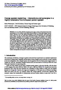
This thesis applies a modelling approach based on energy system analysis, and the applied modelling frameworks, MARKAL and TIMES, use least-cost optimisation in order to analyse the national energy system dynamics over time. While some of the work captures a wider geographical area, all studies comprise policy questions relevant in a Swedish context. The thesis consists of an introductory essay and six stand-alone papers. The main findings of each paper are introduced in the respective abstracts, while the introductory essay instead focuses on the energy system in focus (Sweden), on the model developed within the work leading to this thesis (TIMES-Sweden) and on identifying how national energy system models can be used to support a more robust and transparent energy policy analysis. The papers are integrated into the thesis by putting forward five research questions – of relevance for the included papers and for long-term modelling of the Swedish energy system: Q1) To what extent should cross-border trade of electricity with neighbouring countries be included in a national energy system model? (Paper I); Q2) How can the potential of combined heat and power be represented in a national energy systems model perspective? (Paper II, III, and IV); Q3) How can the potential benefits of Swedish district heating be comprehended in a national energy system model? (Paper IV); Q4) What kinds of ancillary benefits from climate policies can be assessed by national energy system models and how should they be considered in the analysis? (Paper V); Q5) How can TIMES-Sweden (a national energy system models) and EMEC (a national CGE model for Sweden) be linked in order to improve the policy decision-making process at the national level? (Paper VI). The scopes of the embedded papers are on issues of particular relevance for the Swedish energy system; treatment of cross-border trade of electricity within the model, assessing the potential of CHP, capturing district heating in the model, the impacts from domestic CO2emission targets, and finally, the interconnection between macro-economic models and energy system models. National energy system models like TIMES-Sweden generally includes the entire energy system, thus both stationary and mobile energy conversion. The models capture energy conversion processes from primary energy to end use, thus from extraction and imports of energy commodities, via energy conversion into secondary energy carrier (e.g. electricity, district heating and biofuels) and distribution, to end-use processes. The five research questions focus on different parts of the energy system; see Figure 1.
2
Introduction
Policy Instruments
Emissions
Entire Economy
Electricity Heat
IMPORT
EXPORT
International Markets
P R I M A R Y
E N E R G Y
Agriculture
S U P P L Y
Transport Residential
Electri city & Heat
Commercial
Industry
U S E F U L
D E M A N D
Figure 1 The focus of each question and the associated papers put in relation to the national energy system. Blue is the focus of Q1, orange is the focus of Q2, red is the focus of Q3, green is the focus of Q4 and pink is the focus of Q5.
1.3 Central assumptions and delimitations The energy system models used in this thesis are based on either the MARKAL or the TIMES model generator. As an effect of their linearity and partial equilibrium properties, the models contain the following fundamental assumptions (Loulou et al., 2005, Section 3.2):
Profit maximisation and assumptions of self-regulating behaviour of the marketplace – the invisible hand. Thus profit-maximising behaviour of firms and utility-maximising behaviour of households are assumed. While in reality firms and households can have noneconomic preferences, in an energy market perspective this is a reasonable assumption. This will not be further discussed in this thesis.
Perfect foresight: full information both between actors (i.e. no actor sit on unique information) and in time (e.g. the future global prices of oil is known). In reality the future oil and carbon prices are unknown, and so is the resulting technology evolution. The uncertainty of the future is an input to the actual decision process. This can partly be assessed by introducing stochastic programming or by running the model step-wise. Neither of these approaches has been applied or further discussed in this thesis.
3
Introduction
Linearity of investments: all investments in a specific technology will have the same cost per kW independent of the number of instalments or size. In reality, small units are usually more costly than large units (per installed kW) due to economies of scale. Likewise, some technologies are connected with a cost per unit rather than size/capacity (for example emission control). These aspects can to a large extent be captured in the model by defining small and large technologies with a boundary on each group, and this is how the non-linearity of investment is considered in the thesis. In addition, the first unit will be more expensive than unit 1000, due to economies of scale. Other technologies will either be built or not be built, like the case with nuclear plants or pipelines. These can be captured by introducing mixed integer programming. However, this is not applied or further discussed in the thesis.
Outputs of a process/technology are linear functions of its inputs, though many parameters are exponential functions. In reality, the efficiency of some plants will depend on the load factor, i.e. the efficiency is lower at low loads compared with a high plant load factor. This will not be further discussed in this thesis.
TIMES-based models are built on linear programming (LP) but can also include mixed integer programming (MIP) or multi-stage stochastic programming (e.g. Loulou and Lehtila, 2012). MIP is typically used to consider that an event is either happening or not happening (e.g. a large transmission line between two countries). Both MIP and stochastic programming increase the problem greatly and are therefore often only applied on a limited number of activities. Neither of the two is applied in this thesis.
1.4 Outline of this thesis This thesis consists of two parts – an introductory essay and appended papers. The papers are six individual pieces of work and the introductory essay aims to place these papers in a broader context of energy system analysis. The introductory essay is organised as follows: Section 2 describes the research context by giving an introduction to system analysis and concluding with the energy system modelling process. This is followed by a presentation of specific concepts applied in the thesis in Section 3. Section 4 gives an introduction to the Swedish energy system. The TIMES-Sweden model is introduced in Section 5. Section 6 reflects upon uncertainties and model validation. The five research questions are elaborated in Section 7 using the identified energy system modelling process. The main findings are presented in Section 8. Finally, the conclusions are summarized and suggestions for future work are given in Section 9.
4
Methodology – Energy System Analysis
2 Methodology – Energy System Analysis The research introduced in this thesis uses applied energy system analysis, which belongs to/falls under the broader system theory. This section first gives a broad overview of system theory in perspective of the studied systems, followed by a more detailed description of the applied system approach. Energy system analysis is then introduced followed by an overview of how energy system models can be classified. Finally, an energy system model process is presented.
2.1 Systems theory ‘A system is a set of objects together with relationships between the objects and between their attributes.’ O R Young (1964) In 1950, Ludwig von Bertalanffy introduced the theory of open systems in physics and biology as a contrast to the second law of thermodynamics. In Bertalanffy (1950), he argues that the second law of thermodynamics is only true for closed systems, while most systems interact with their surroundings. Thus, he concludes that most systems can therefore not be studied in isolation. He also emphasises that different sciences interact. For example, physics can help explain biology (e.g. gravity defines how big an animal can be) and by understanding biology better new views open up within physics (e.g. osmosis). The ideas were later further developed into general system theory (GST). ‘You cannot sum up the behaviour of the whole from the isolated parts, and you have to take into account the relations between the various subordinate systems which are super-ordinated to them in order to understand the behavior of the parts’ (von Bertalanffy, 1968). Those thoughts are repeated and reframed through the literature of system analysis and system thinking (e.g. Churchman, 1968; Checkland 1981; Luhmann, 1964; and Jackson, 1991). A system may be defined as a set of elements standing in interrelation among themselves and with the environment’ (von Bertalanffy 1968). According to Churchman (1968), system analysis is based on the conception that analysing a system is more complex than analysing each part of the system individually and a central point is to distinguish between the system and its surroundings – the system environment. Churchman (1982) distinguishes between bounded and unbounded system thinking. Bounded system thinking occurs when assuming that there are problems that can be analysed in isolation and that have possible solutions (Churchman 1982, p.6). Churchman argues that most problems related to humanity include all other problems and that we therefore need an ‘unbounded system approach’ which also should include studies of the ethics of humanity, not just within the studied system but universally, i.e. every problem is a part of all other problems (Churchman 1982, p.8). Niklas Luhmann, who made important contributions in the field of social systems (e.g. Luhmann, 1995), argues that the system surroundings are more complex than the system itself and that the complexity in the surroundings needs to be simplified in order to enable a meaningful analysis of the system. He continues by stating that the systems do not really 5
Methodology – Energy System Analysis communicate with their surroundings but can replicate and take in the surroundings as the complexity reduces. Systems interpret their surroundings based on their own preferences and logic, and only the features in line with and recognised by the system will be considered. Luhmann calls this resonance and this is the way a social system is affected by the surrounding society and the overall development of society (Ingelstam, 2002). When looking at a specific system, it is therefore more important to identify how the specific system looks at the surroundings rather than how the surroundings actually function. There are many different types of systems, systems that demand different approaches in order to be understood. One way of categorising different types of systems is by different system families. Ingelstam (2002) defines five different system families (see Figure 2), inspired by Luhmann’s grouping of systems. Ingelstam and Luhmann share three system families, machines, organisms and social system. When Luhmann defines a psychic system family, Ingelstam instead defines one socio-technical system family representing the interaction between society and the technology and one ‘technology, environment and society’ family representing the environment and limited resources. Research on socio-technical systems is also referred to as science, technology and society (STS)1.
Figure 2 The definition of system families as fundamental bricks in understanding the overall system (Ingelstam 2002, p. 28). The appended papers look at three different systems: the Swedish energy system (Papers IV, V and VI), the Nordic power system (Paper I) and the European energy system (Papers II and III). Common for all three systems is that they can be described as large socio-technical systems. A large technical system (LTS) is a system or network of enormous proportions or complexity (Hughes, 1983). According to Ingelstam (2002), a socio-technical system consists of three parts: i) technical material components and their relations (e.g. efficiency of the plants and energy flows), ii) social components and relationships (e.g. the demand for energy service and the competition’s willingness to pay) and iii) the interaction between the technical
1
The abbreviation STS is in the literature used both for science, technology and society and for socio-technical systems.
6
Methodology – Energy System Analysis material and the social components (the competition between technologies and the evolution of different technologies). In a socio-technical system, the technical parts and the social parts of the system are tangled into each other and the system cannot be fully understood by only looking at one part. Distinguishing between the technical and the social system is not straightforward since they are merged into one another. Hughes, a historian of technology and one of the pioneers within large technical systems (LTS) theory, describes this as a seamless web in Hughes (1986). Furthermore, he describes how historians of science and technologies have changed from a non-contextual or ‘internalist’ approach – where each step of the invention of an artefact was presented in a chronological narrative without any explanation of how the changes occurred – to seeking the explanation for change by putting the evolution into a ‘context’, which is divided into groups like social, technology, science, politics and economics. Hughes (1986) instead argues for a system approach, since the artefact and the context interact. The context affects the artefact and the artefact affects the context. Categorisation of the context into hard defined groups should be done sparsely when the interactions are more complex and reach into each other like a seamless web. A theory around social construction of technological systems (SCOT) was presented by Bijker, Hughes and Pinch (1987). In Hughes (1983), the history of the electrification of the western society is told based on the LTS theory. Summerton (1992) looks at Swedish district heating by applying LTS and actor-networks theory. Kaijser (1995) tells the history of the Nordic electricity system evolution using an LTS approach. The past development of the Swedish power system can also be understood by addressing the underlying process in certain central decisions, as in e.g. Anshelm (2000) and Sandoff (2002). Anshelm (2000) describes the discourse of the Swedish public debate on nuclear power from a political science perspective. Sandoff (2002) analyses the competitive advantage in Swedish electricity retail companies by looking at the local investment process. The first comprehensive study on the future Swedish energy system was Solar or Uranium, where Lönnroth et al. (1978) compare two different future Swedish scenarios, one with solar and one with uranium. The authors do not claim to use a special methodology; the complexity of each energy scenario is instead assessed from different angels and the interaction both within and between technology and society is included in the analysis. For example, they discuss the importance of not only evaluating the technology features but to also consider whether society can handle the chosen technology and how the chosen technology might affect the development of society. Another way of assessing the future is by using energy system models, as applied in the present thesis and further described below.
7
Methodology – Energy System Analysis
2.2 The systems approach ‘Systems are made up of sets of components that work together for the overall objective of the whole. The system approach is simply a way of thinking about these total systems and their components.’ C. West Churchman, (1968, p. 11) The research in this thesis is largely built on the approach discussed in Churchman (1968). The title of his book and the title of this section is the systems approach instead of system analysis, as it describes a way of thinking rather than a straightforward methodology. According to Churchman (1968), system thinking starts when one for the first time looks at the world through someone else’s eyes. System thinking leads to the discovery that each world view is extremely limited. Churchman writes that there are no ‘real’ experts in system thinking – the public always knows more. The systems thinkers’ work is instead to find out what ‘everyone’ knows and put it together. In this process it is important to examine both the system’s real aim and the management’s goal with the system. The management can be described as the one who can set targets and steer the overall system. Those vague objectives are then translated into specific performance measures for the system as a whole. Performance measures, as the name implies, should be measurable. The role of the system analyst is to structure the problem, while the role of the management is to set targets for the components, allocate resources and control the system performance. To support the ‘thinking processes, it is useful to create a model. A model is a simplification of reality where the main components and parameters of the problem are represented. The process can further benefit from building a computable model of the problem, in particular linear programming (LP) models (Churchman 1968, p. 61). Even though all problems are not solvable with a computable model, Churchman argues that the way of thinking inherent in LP models helps to structure and solve the problem. Finding the following structure, inspired by LP models, where Churchman describes which aspects need to be identified when approaching a system is therefore no coincidence: 1. The system's overall objectives and performance measures for the system as a whole, 2. The system's components, i.e. their activities, goals and performance measures, 3. The system’s environment, i.e. the fixed constraints that cannot be influenced, 4. The system's resources, i.e. resources that the system can use, and 5. The management of the system, i.e. the decision makers who make the plans for the system. Churchman does not like the idea outlining a system boundary (Churchman 1968, p 35-36). Instead, he wants to distinguish between the parts that belong to the system and should be included in the objective function of the LP model and the parts that belong to the system environment and should be defined as boundaries in the LP model. Everything that from a system’s point of view is ‘fixed’ or ‘given’ is by Churchman defined as the system environment. These are things and people whose characteristics and behaviour are less likely to be 8
Methodology – Energy System Analysis affected by the system in focus but still have an impact on meeting the objective (Churchman 1968, p. 36). Despite the fact that some things can be excluded from the system, it is still easy to consider more and more things as part of the system, to the degree that the system becomes too complex and thereby impossible to solve. On the other hand, if we simplify too much, we might miss important factors with significant impact on the studied system, i.e. what Churchman in ‘The Systems Approach and Its Enemies’ calls the ‘environmental fallacy’ (cited in Gigch 2006, p. 23-24). Some of Churchman’s opponents accuse him of diminishing the analytical challenge and of being too optimistic about the usefulness of models, especially his suggestions that even behaviour can be incorporated in the models by quantifying it. Nevertheless, he too acknowledges the limitations of models. Model results can never be better than the input used. Even though it is tempting to use historical demand as a basis for estimating future demand and thereby assume that the future will be like the past, this is a poor research strategy from a systems point of view (Churchman 1968, p. 127). This can be dealt with by using crossdisciplinary science and mainly using models to get a holistic view of the system. Another limitation of the system approach is that ‘the system is always embedded in a larger system’ and what is optimal for the selected and studied system might not necessarily be optimal at a higher system level (Churchman 1968, p. 76). He stresses the importance of avoiding oversimplification even though a model can never capture the full details of a system (further discussed under uncertainties in Section 6.5). Churchman also raises concerns about the impossibility of being objective when having insights about the details. This is later brought up in e.g. Churchman (1982, p. 17), where he emphasises the importance of a high moral of the system planner and of focusing on the real problem, e.g. ‘kids are starving in great numbers, damn it all’. Churchman’s system approach is central in this thesis. My main concern with it, though, is the freedom of choice of method or rather mixes of methods (e.g. Churchman 1968, Chapter 11). There is an immediate risk of starting with a specific method/model to support an underlying purpose, either deliberately or unconsciously, instead of starting with the problem and then selecting the appropriate method/model. This flexible use of methods can also cause confusion in the scientific community, where the system analysts seem to use a patchwork of methods from different research fields. They do not seem to be strictly objective and are therefore not always deemed to be scientific. However, this risk exists within all fields of science, which was pointed out in Churchman (1961, p.14): ‘The scientist decides what to study; he decides what model is adequate within which to pose his problem; he decides how, when and where to make observations, he decides when to accept or reject a conclusion’. All those decisions can have impact on the results. The main difference between studying sociotechnical system and studying specific engineering processes is that the socio-technical system includes human beings. Human beings, with different fundamental perception and values (moral, ethic, principles), who make different kinds of decisions. Even if those parameters can be measured for individuals, those findings would be difficult to generalize and in addition those parameters are likely to change over time (further discussed in e.g. Churchman 1961; Ackerman and Heinzerling 2004). How, and to what extent, individual decisions should be included in the analysis will depend on the scientific problem. Different 9
Methodology – Energy System Analysis methods/models are needed to solve different kinds of problems. Used wisely, the freedom of methods/models is therefore also the strength of system approach. Methods/models should mainly be seen as tools to solve the overall objective. The focus should be on identifying the objective. Churchman (1968) describes the systems thinker as someone searching for gaps who needs better methods/models in order to analyse a complex system. What is more of an actual concern with the approach described in ‘The systems approach’ (Churchman, 1968) is the undertone that it always is possible to find an appropriate (mathematical) method to solve all problems with system approach. When reading ‘The systems approach’ it is also easy to get the impression that it is possible to identify one or at least a set of ‘optimal solutions’ to the problem. He does state that the best solution not necessarily can be implemented, but one get the impression that it is possible to identify an optimal solution that the outcomes from the analysis can be compared against. I believe this is misleading as all analysis, also the ‘optimal solution’, includes generalisations made by humans, i.e. simplifications. Churchman himself also seem aware of this, in Churchman (1968, p.35) states the following: ‘It is sheer nonsense to expect that any human being has yet been able to attain such insight into the problems of society that he can really identify the central problems and determine how they should be solved. The systems in which we live are far too complicated as yet for our intellectual powers and technology to understand.’ Nevertheless, despite all uncertainties, despite that there never will be one ‘true’ way of looking at the problem and despite that we will never fully understand the systems we live in, it is still valid to approach the system. We will always experience new aspects of the systems and of their components. The core of system thinking is both confusion and enlightenment. ‘The two are inseparable aspects of human living’ (Churchman 1968, p. 231).
2.3 Energy system analysis ‘Present energy systems are the result of complex country dependent, multi-sector developments.’ GianCarlo Tosato (2009) When system analysis is applied to the energy sector, it is named energy system analysis and is ultimately about managing limited resources – allocation of limited sources such as biomass and monetary resources. The development of the national energy system will depend on multifaceted decisions and conditions, of which some are country dependent and some are universal. The government can be defined as the management of the national energy system, as they define the main rules by imposing policies, providing infrastructure and maintaining markets while the decisions about different energy solutions are made by stakeholders and citizens. These decisions are described by Tosato (2009) as based on the 4Es – energy, engineering, economic or environmental – and the sum of all decisions shape the energy system. Even though each of these decisions could be described from a rational point of view, and thereby possibly be represented and described in a model, it is more difficult to find 10
Methodology – Energy System Analysis rationality in the overall system (Tosato, 2009). The reason is that decisions are also based on values and irrationality, which are difficult to capture in an aggregated model as they differ greatly between individuals and can change from one year to another due to e.g. changes in society. Hence, besides the 4Es, the development of the energy system will depend on the social system and the behaviour of individuals. Preferences, interaction and people’s behaviour are difficult to generalise and represent in models, especially in large aggregated models. Nevertheless, this does not imply that they can be ignored, but might need to be assessed outside the model. The 4Es are further described below.
2.3.1 Energy – from primary resource to end-use services The energy system can be described as a sequential series of linked steps, alternating commodities with energy conversion and transformation processes that ultimately result in the delivery of goods and services, visualised in Figure 3 (Tosato, 2009, p.2). In order to analyse the system, it is important to distinguish between different kinds of energy forms. Energy commodity, or energy carrier, is used by Eurostat both when referring to fuels, heat and power, where fuels are substances that can be transformed into electricity and/or heat (Eurostat, 2004). Primary energy is the pure energy form that exists naturally and thus has not been subjected to human-imposed conversion or transformation. Primary energy can also include energy forms that are based on man-made materials without alternative use. Secondary energy is the form of energy found after the conversion or transformation of primary energy. Final energy consumption is by Eurostat defined as energy commodities delivered to consumers for activities that are not defined elsewhere in the balance structure (fuel conversion into electricity and heat or fuel transformation are example of activities that are presented in other parts of the energy balance). Final energy commodities are in the Eurostat statistics considered to be consumed and not transformed into other commodities, and thus disappears from the account (Eurostat, 2004). In the recent energy efficiency directive (Directive 2012/27/EU), final energy consumption is defined as ‘all energy supplied to industry, transport, households, services and agriculture. It excludes deliveries to the energy transformation sector and the energy industries themselves.’ Another way of expressing final energy consumption is an energy commodity supplied to the final consumer’s door. The next step in the energy chain is useful energy, which Häfele (1977) defines as the energy available to the consumers after the final consumer energy conversion, i.e. final energy consumption minus conversion losses.
2.3.2 Engineering – technology efficiency and system efficiency The efficiency of the system will depend on the efficiency of the individual technologies. Technologies are both energy conversion technologies with the main aim to transform energy from one form to another (e.g. biomass to power and heat) and processes that use energy to produce a good (e.g. steel) or service (e.g. to be transported from A to B). In addition there are technologies that transport the energy commodity from the producer to the users. Technologies can be divided into demand-side technologies (including the possibility to define energy conservation measures), supply-side technologies (including conversion into secondary energy carriers), resource extraction technologies, and infrastructure technologies.
11
Methodology – Energy System Analysis
2.3.3 Economics – the value of energy systems The cost of supplying enough energy to meet a specific demand for goods and services depends on the entire energy chain – from extraction, via energy conversion and distribution to delivery. Only costs paid by actors within the energy system will be included. Thus, in a national perspective the import of energy commodities will be measured by the costs at the border and the export will be considered as revenues to the system. The costs of energy conversion and energy networks are associated with capital or investments costs as well as fixed and variable operation and maintenance costs. In addition, implemented taxes and subsidies will have an effect on the overall cost of delivering energy to meet a specified demand for goods and services. When comparing different policy alternatives, the differences in energy system cost can tell us something about the cost of implementing a certain policy. However, these are the costs of supplying the energy and no do include other possible effects on other parts of the economy (i.e., so-called general equilibrium effects). Worth mentioning is also that in an energy system perspective taxes are looked upon as a cost and subsidies as an income. In the best of worlds, taxes exist to compensate for negative externalities from the generation of energy; they are thus correctly accounted as a cost, while in practice they also contribute to the government budget. Subsidies are instead a burden for the government’s finances, while they reduce the specific costs of meeting the energy demand.
2.3.4 Environment – pollution and other environmental impacts All energy use has some degree of environmental impact. The conversion of energy from one form to another is connected with a number of environmental effects both during the extraction of energy sources (e.g. CH4 emissions from extraction of fossil fuels and radiation from extraction of uranium) and the manufacturing of technologies (e.g. toxicants and chemicals from the manufacturing of photovoltaic cells), and combustion of both fossil fuel and biomass is associated with the emission of CO2 and air pollutants such as nitrogen oxides (NOX), particles, sulphur dioxide (SO2) and volatile organic compounds (VOC). In addition, the extraction of energy can affect the biodiversity, as noted in the case of crops for biofuels production in particular. Likewise there are conflicts in land-use between biofuels and food production. However, the conflict is complex the competition of land-use might not be between food production and biofuels but rather between biofuels and animal feed (Hansson et al., 2006). Another area of conflict is the use of water both when growing biomass, when cleaning and cooling large-scale solar plants and when cooling thermal plants (also includes nuclear plants). Environmental impacts from wind power are reviewed by e.g. Dai et al. (2015). There are also land-use conflicts in relation to areas for recreation and tourism and the lifestyle of indigenous peoples. Consequently, there is no such thing as completely ‘clean’ energy sources.
12
Methodology – Energy System Analysis
Figure 3 A schematic energy system with examples illustrating common energy flows used in energy system analysis. Source: Tosato, 2009 (Figure 4-1).
13
Methodology – Energy System Analysis
Figure 4 A simplified schematic representation of energy flows to meet the demand for energy services, illustrating the losses in each conversion step. Source: Häfele, 1977 (Figure 2).
2.4 Energy system models ‘Even if models are inaccurate forecasting devices, they are useful today and they could become even more useful in the near future. First, because there is evidence to suggest that humans, being biased forecasters, are even worse than models. Second because models besides forecasting have another very important use, as tools for analysis. They can assist the human brain in the process of rational analysis and synthesis, by broadening its capacity of doing so, by formalizing its judgemental procedure and by formulating a logical consistency framework.’ Samouilidis (1980) In line with Amerighi et al. (2010), a model is hereby defined as ‘quantitative mathematicallybased methodology’, whereas a procedure instead is defined as a ‘sequence of codified and systematic steps’ shared by the scientific community to examine a specific topic. Early publications with energy models focus on the power sector, due to an identified growing demand for electricity in combination with power plants requiring long-term planning due to large investments and long lead time between decisions and operation. Optimisation models were commonly used as decision tools by the power utility in order to determine the optimal investment strategies (Samouilidis, 1980). The first optimisation models were, in general, linear programming models. These are still commonly used and are today supplemented with a variety of other models such as stochastic programming, mixed integer programming and system dynamic models.
14
Methodology – Energy System Analysis Energy models can be classified in many different ways. Samouilidis (1980) refers to three groups; ‘open loop demand/supply’ models (exogenous demand), ‘energy closed loops’ models (calculates a partial equilibrium) and ‘energy-economic closed loops’ models (the energy economy interaction). Energy models are by Samoulidis (1980) identified to have some typical characteristics, namely how the demand side is included in the model (useful energy or final energy), the ‘degree of details’ (the number of technology options and the number of user segments), the ‘length of the planning horizon’ (10 to 60 years) and the ‘relation to time’ (static or dynamic). Larsson and Wene (1993) instead classify energy models based on decision level. In IPCC (1996), the models are structured according to characteristics, structure and external assumptions. In contrast, Pandey (2002) classifies models based on ‘paradigm’ (analytical approach), space (geographical coverage), sector coverage and time. Within the ATEST project (Amerighi et al., 2010), a literature review finds the following criteria commonly used when classifying energy system models: main aim of the model, theoretical platform, geographical coverage, time dimension (time horizon and granularity), sectoral coverage, technology coverage, economic description, ‘capability to analyse policies’, data requirements and ‘linkage possibilities and needs’. Pfenninger et al. (2014) discuss energy system models of relevance in the face of stringent climate policy, energy security and economic development concerns and divide energy models into four groups: energy systems optimisation models, energy systems simulation models, power systems and electricity market models, and qualitative and mixed-methods scenarios. They point at the fact that energy system models have been developed under several decades, and that we now face partly different modelling challenges, i.e., liberalised markets, intermittent power etc. Nevertheless, they identify that energy system models form the basis for policy analysis in many countries and regions, and that energy system models in combination with other models can help contribute in to meet energy challenges of the twenty-first century. Energy system models are also referred to as comprehensive energy system engineering models (ESEMs). Such modelling tools are used for analysing future technology options from a system perspective. Examples of ESEM used at national level and higher are models based on MESSAGE2, EFOM3, MARKAL4 and TIMES5 model generators. The generators can be used for creating models with different sectoral and geographical scope. MARKAL and TIMES are the ones that have been used in Sweden. The first MARKAL model applied on Sweden was developed by Per-Anders Bergendahl at the Department of Economics, University of Gothenburg (Bergendahl and Bergström, 1981; Tosato et al., 1984, Chapter 6.11). Thereafter different MARKAL-based regional models were developed and used for local energy/environment planning (e.g. Wene and Rydén, 1988; Rydén et al., 1993). A Swedish energy system model at a national level was developed at Chalmers University of Technology and applied in e.g. Larsson (1993) and Larsson and Wene (1993). The model was later developed to also include a MACRO module, i.e., the Swedish MARKAL-Macro model,
2
MESSAGE is described in Messner (1984). EFOM is described in Van der Voort (1982). 4 The MARKAL model generator is described in Fishbone et al. (1981). 5 TIMES is an acronym for The Integrated MARKAL-EFOM System, and the model generator is described in Loulou et al. (2005). 3
15
Methodology – Energy System Analysis documented by Nyström and Andersson (1995). A MARKAL model of Sweden, Denmark and Norway was developed to consider the impacts of cross-border trade (Larson et al., 1998). The model was further developed to also include Finland, creating the MARKAL_Nordic model (e.g. Unger, 2000; Unger and Alm, 2000). MARKAL_Nordic focuses on the Nordic stationary energy sectors and has been extensively used for official Swedish medium and long-term energy analysis (e.g. SEA, 2003; Unger and Ekvall, 2003; Unger and Ahlgren, 2005; Profu, 2010; Profu, 2012). In Börjesson and Ahlgren (2010) a regional MARKAL model is developed and linked with MARKAL_Nordic to compare the cost-effectiveness of biomass gasification technologies and conventional technology alternatives in a regional district heating perspective. Within the Nordic ETP model, a basic Nordic TIMES model was developed based on IEA’s ETP TIMES model with a focus on the power sector. TIMESSweden was developed in work leading to this thesis and two different EU projects, NEEDS6 and RES20207, and captures the comprehensive Swedish energy system. The model is further described in Section 5. Besides MARKAL and TIMES-based models, there are a few other Swedish models with a national focus. A simplified energy system model of Sweden based on OSeMOSYS is presented in Saadi Failali (2013). MODEST, a model similar to MARKAL, was developed by and documented in Henning (1999) and is today generally applied at the local or regional level (e.g. Karlsson et al, 2009; Åberg and Henning 2011). Computable general equilibrium (CGE) models for Sweden (a small open economy) often include the electricity and fuel production as separate sectors, starting with Bergman (1982) and later the EMEC model. EMEC is short for ‘Environmental Medium Term Economic Model’ and is developed and maintained by the National Institute of Economic Research (Östblom, 1999; Östblom and Berg 2006). CGE models differ from energy system models, but they are both used for analysing energy and climate policy analysis. EMEC focuses on the interaction between the economy and the environment, while MARKAL_Nordic and TIMES-Sweden focus on the interaction between the energy and the environment.
2.5 Energy system modelling process ‘System Analysis does not give you a plan for the future, but it helps you to become aware of and to understand quantitative relationships between different parts and different times of a complex system under widely varying conditions. It also helps you to understand contingencies and to compare risks.’ Sigfrid Wennerberg (Preface in Tosato et al., 1984)
6
‘New Energy Externalities Development for Sustainability’ (NEEDS) was a research project of the European Commission in the context of the 6th Framework Programme, Research Stream 2a ‘Modelling internalisation strategies, including scenario building’. Website: www.needs-project.org.
7
‘Monitoring and evaluating the RES directives implementation in EU27 and policy recommendation for 2020’ (RES2020) was funded by the Intelligent Energy Europe research programme. Website: www.cres.gr/res2020.
16
Methodology – Energy System Analysis
Even though energy system models are often used for long-term forecasting, e.g. estimating the future prices of electricity, the most common aim is to explore different alternative developments and to get a deeper understanding of how the energy system can develop over time under different sets of assumptions, i.e. different scenarios. Common for many practitioners (e.g. Churchman, 1968; Samouilidis, 1980) is their attitude towards the model – the problem goes beyond developing a mathematical model and the quantitative results. The work with models – in a system approach – also includes the process of identifying how the system could be represented in the model and a critical assessment on how the results can be brought back to reality and their impacts on the actual policy decisions. The process of working with energy system models can be described as three steps, illustrated in Figure 5, inspired by Clas-Otto Wene8.
Figure 5 The system analysis approach applied on the energy system modelling process. First the ‘real’ system is simplified and conceptualised into a model (step 1). Then all assumptions are sorted in a mathematical model and the algorithms solved (step 2). Finally the model results are interpreted and conclusions drawn about the future energy system (step 3).
8
Clas-Otto Wene, professor emeritus, professor at the Energy System Technology unit, Chalmers University of Technology, 1978-1998.
17
Methodology – Energy System Analysis First the ‘real’ system is simplified and conceptualised into a model (step 1). Then, all assumptions are sorted in a mathematical model and the algorithms solved (step 2). Finally, the model results are interpreted and conclusions drawn about the future energy system (step 3). The process of identifying the components of the system and their relationships is seen as important in order to understand the overall problem. Churchman (1986, p.29) outlines five basic ‘considerations’, all important when approaching the system with the aim of conceptualising the reality into a model; see Table 1. It is not a coincidence that the five considerations are very similar to how a LP model is structured. Churchman argues that the way of thinking inherent in LP models helps structure and solves the problem (further described in Section 2.3). Also Tosato (2009) identifies important bricks that need to be defined in order to describe the system, but with different terms and with a focus on aspects needed when describing an energy system; see Table 1. Table 1 Identifying basic parts in energy system modelling. Identified Energy System Modelling Process
‘Modelling’ Operations Research
System Analysis (Churchman 1968, p. 29-30)
System Analysis (Tosato, 2009)
Define the objective – identify what determines the coefficients in the objective function
1. Identify the system’s overall objectives and performance measures
Scope of the analyses
Identify the variables
2.Identify the components of the system (their activity – their objectives and their performance measures)
Time frames: time horizon and time granularity Components (elements, parts) Connections, interdependencies and chains
Define the problem’s constraints – identify the limitations and boundary conditions
3.Identify the surroundings – the system’s environment and fixed constraints that cannot be affected 4.Identify the resources of the system
Boundaries
Define the LP problem
5.Identify the management and the consumers of the system
Solve the problem (optimisation)
Solve the problem
Solve the problem
Interpret the solution
Interpret the solution
Interpret the solution
STEP 1: Conceptualisation
STEP 2: Model STEP 3: Interpretation
STEP 1: Conceptualisation The first step in the energy modelling process comprises the translation of the ‘real’ system into a model by establishing a conceptualised description of the system. An energy system can be described by physical flows of energy carriers, materials and emissions. One way to illustrate the interaction of the flows is to draw a graphical representation, a ‘map’, of the studied technical energy system, a so-called reference energy system (RES). The concept of 18
Methodology – Energy System Analysis RES was introduced by Marcuse et al. (1976), and an example is shown in Figure 6. Beside the techno-economic parameters of the TES, a number of factors affect the long-term development and investment pattern. Wene and Rydén (1988) identify four boundary conditions that describe the system environment: useful energy demand, technology development, energy resources and physical environment. Tosato (2009) describes the energy system as having four dimensions: energy, engineering, economic and environmental. When deciding which part of the energy system to include or exclude and when deciding how included parts should be described, the system’s management and consumers first have to be identified. The management is in control of steering the system and the consumers are the ones using the services. The level of detail will depend on the studied question and specific assumptions will vary between scenarios. STEP 2: Model The second step of the energy modelling process is the model itself and deals with the model algorithms rather than identifying connections within the energy system (this belongs to step 1). Models that include the entire or major parts of the technical energy system and describe the energy conversion chain from primary energy source, via conversion and transmission technologies, to final or useful demand represent comprehensive energy system engineering models (ESEMs), also labelled energy systems models. STEP 3: Interpretation – interpreting results and drawing conclusions The third step of the energy modelling process is the interpretation of the results and the drawing of conclusions. There is no straightforward approach for interpreting the results, since the approach will depend on the studied question. Nevertheless, some issues need to be addressed in order to draw robust conclusions. One important part of the results analysis is a ‘reality check’ of the result, which is useful both for improving the understanding of the model and gaining acceptance for the results. This does not imply that the results should correspond with the past or with our expectations, but rather that they are explainable. When drawing conclusions, it is also important to explain the results with respect to the defined rules (the indirect model assumptions) and the assumed input to the model. Are the results derived from the cost-minimisation or are they a consequence of the assumptions? It is also important to pay attention to how the result differs from the reality due to the specific model (see Section 1.3). E.g., the model is based on cost-minimisation, i.e. minimise the total system cost to meet the given demand under certain boundaries. In reality the decision preferences differ between individuals and can apart from costs include environmental concerns and neighbours´ interactions. Which impact does this limitation have on the results? It is also important to pay attention to aspects not captured by the model. In these cases additional information need to be added to the quantitative analysis and/or the quantitative modelling results can be used as an input to a qualitative analysis. This is especially the case in areas for which non-economic or technical aspects are assumed to have a big impact on the outcomes. It can also be the impacts of the energy on the economy or society that are not captured in the model, e.g. the impacts of the resulting energy mix on the remaining economy (see Paper VI). 19
Methodology – Energy System Analysis When looking far ahead into the future, the resulting energy system (from the model) might look very different from today. In these cases it can be important to reflect upon the consequences of different energy systems for the overall society? Lönnroth et al. (1978, p.215) look at the implication on the society from two different angles, by asking two different questions. What does a specific energy system request from the society? How will the development of the society and its ‘spirit/atmosphere’ be affected by certain choices of energy system? At this time, Sweden were still deciding if proceeding with the nuclear program or not, and Lönnroth et al. (1978) focused on the choice between nuclear and solar energy. The first question therefore concerned whether a small country was able to handle and keep up with very advanced technologies, such as nuclear power. The second question concerned whether some trends in the society, e.g centralisation, individualisation individualistic, elitist society would be reinforced if choosing a certain energy technology. Today, there is a larger focus on having many different energy sources. A more relevant approach to the first question could then be to examine how specific technologies can be integrated into existing market structures, thus representing a deregulated energy market also including people’s preferences (will certain technologies be chosen?). If certain technologies are found to not fit into the present market structures, the analysis should include what changes that are needed in order for the technology to assimilate. And, more important, would this change in market structure be desirable? A related aspect is the lock-in effect, described in a climate policy perspective in (Unruh, 2000; Unruh, 2002; Unruh and Carrillo-Hermosilla, 2006). An example of a lock-in effect from the past is the choice between alternating current (AC) and direct current (DC). AC, which facilitates transmission of electricity from a distant source (like hydro power) to the demand centres, was chosen. Had DC instead been chosen, a possible outcome could have been that the demand centres – cities – would have been located closer to the energy resources, and centralised small-scale power plants might have been the dominant technology instead of large-scale hydro, nuclear or coal plants. When looking at the future energy system, we are facing a structural change as regards vehicles; will the transport pattern differ if a country promotes plug-in hybrid vehicles rather than electric vehicles? Can this also have an impact on the choice between public versus private transportation? Consequently, it might change the underlying demand assumptions in the model. STEP 1-2-3: An iterative process The energy system modelling process is not a sequential process starting at point 1 and ending at point 3, but rather an iterative process going back and forth between the different steps. In order to attain robust conclusions about the future system, it is necessary to re-visit the in-data (step 1) when checking the consistence and coherence of the results with regard to the ‘real’ system (step 3).
20
Figure 6 The figure shows a reference energy system (RES) with a focus on the residential sector. A RES is a graphical model of the technical energy system with its physical flows of energy, energy conversion technologies and boundaries. The energy demand can be described with final or useful demand. Final demand refers to the amount of a specific energy carrier used, while useful demand refers to a need of a specific service, such as keeping an indoor temperature of 20 degrees Celsius.
Methodology – Energy System Analysis
21
Concepts Applied
3 Concepts Applied This section describes concepts applied in this thesis. The intention is not to give an overview of each concept, but rather to present how each concept has been interpreted in the text.
3.1 Potential When analysing the potential of for example an energy commodity, the diffusion of a technology or the reduction of greenhouse gases (GHG), it is important to acknowledge that there are different kinds of potentials, each representing a category of barriers. IPPC (1996) defines three different potentials for reducing GHG or improving energy efficiency: technical, economic and market potential. The technical potential is the amount that can be reduced/ implemented ‘by using a technology or practice in all applications in which it could technically be adopted, without consideration of its costs or practical feasibility’. The economic potential is the amount that can be cost-effectively reduced/implemented in absence of market barriers. Thus, some of this potential might need additional policies and measures to remove market barriers in order to materialise. The market potential (also called currently realisable potential) is the amount that can be reduced/implemented ‘under existing market conditions, assuming no new policies and measures’ (IPPC 1996, Appendix E). DOE EERE (2006) looks at the potential of different energy sources and stresses the difficulties of comparing quantified potentials from different studies due to differences in assumptions and methods. It is concluded that the fact that different technologies and energy commodities face different kinds of conditions, thus requiring different approaches. This could be the reason why it is difficult to find a clear-cut definition of the different kinds of energy potentials. Even so – or because of that – there is a need to be transparent in the definition applied whenever using the potential. Lopez et al. (2012), and recognising and defines four different types of potentials: resource, technical, economic and market; see Figure 7. Those definitions are useful, but the market definition is not homogeneous with what can be captured in energy system models, when market potential is defined based on both limits due to regulations, limits due to investor response to policies and limits due to regional competition with other energy sources. The first two concern organisational obstacles in the market dealt with in e.g. management science, while the two latter are usually described in monetary values and can be assessed in a partial equilibrium model (e.g. can be captured in energy system models such as TIMES/MARKAL). There are policies in place to remove socalled market failures, such as information asymmetries and externalities. Thus, in a perfect world, implemented policies have compensated for the market failure and have removed the market barrier. One could therefore argue that implemented policies instead of being included in the market potential (as in Figure 7) should be included when estimating the economic potential.
22
Concepts Applied
Resource
Resource potential: Physical constraints, theoretical physical potential, energy content of resource
Technical
Technical potential: System/topographic constraints; land-use constraints; system performance.
Economic
Economic potential: Projected technology costs; projected fuel costs;
Market
Market potential: Regulation limits; investor response; policy implementation/impacts; regional competition with other energy sources.
Figure 7 Different levels of potential.
3.2 Scenarios Systems that are well understood, and where complete information is available, can be predicted with some precision. This can be the case within physical sciences and hence their future states can be predicted. However, the future energy system will depend on many unpredictable assumptions, such as user behaviour (e.g. time in the shower) and investment preferences (e.g. environmental concerns), making the future outcome impossible to predict. The understanding of possible future developments of such complex systems can instead be assisted by a set of scenarios. Scenarios are images of alternative futures, and should not be understood as forecasts or forecasts. A scenario could instead be thought on as a particular image of how the future can unfold. Scenarios are useful tools for investigating alternative future developments and their implications, for learning about the behaviour of complex systems and for policy making. (Nakicenovic et al., 2000). There are two different approaches on how to address scenarios, normative and descriptive scenarios. Normative (or prescriptive) scenarios are explicitly values based and teleological, exploring the routes to desired or undesired endpoints (utopias or dystopias). Descriptive scenarios are evolutionary and open-ended (the choices given to the analysis will determine the end), exploring possible ‘likely’ paths into the future (IPCC 2000, Section 1.2). Many scenarios have elements of both approaches. Likewise, there are different ways to identify the paths or routs – by storytelling/storyline (qualitative), by models (Quantitative) or by a mix of the two. Nakicenovic et al. (2000) emphasises on the fact that no scenarios are ‘value free’. Even though researchers have the ambition to be objective they live in the present paradigm, see discussion in Section 2.2. This is important to have in mind, and point at the importance to occasionally do explorative scenarios, scenarios which might seem unrealistic at the time being.
23
Concepts Applied Due to the fact that the energy systems change slowly, energy scenarios need to have a long time horizon. Nakicenovic et al. (2000), argue for using a time horizon of about 100 years in order to identify a sustainable energy scenario, and with 20-30 year time horizon to identify which policy instrument to implement in order to get to the next phase.
3.3 Externalities ‘An external cost, also known as an externality, arises when the social or economic activities of one group of persons have an impact on another group and when that impact is not fully accounted, or compensated for, by the first group’, (ExternE, 2006). When a company plans for a new power plant, it considers the costs and the benefits actually paid for – the so-called private costs. Still, the company’s activity can have an effect on a third party, which is not considered in the cost-benefit assessment – so-called externalities. These can be both positive (external benefits) and negative (external costs) (Baumol and Oates, 1988). Externalities do not necessary have a specific monetary value. Effects with a direct effect on the price of goods and/or services are easier to assess than effects related to people’s preferences that are not revealed in existing markets. For example, if the real estate price decreases in a neighbourhood due to a firm’s activity, it can to some degree be measured in reduced economic value. It is more difficult to measure the impact of a neighbour playing loud music. One way to find out people’s preferences is to ask how much people would be willing to pay (maximally) to avoid the impact, or how much people would need (as a minimum) in compensation for accepting the impact. Churchman (1982, Chapter 8) problematises the challenge of measuring human values and peoples’ preferences, emphasising that all findings represent individuals’ preferences put in a specific environment. ‘The people that we’re theorising about exist in only one rather odd part of humans’ minds’. Still, Churchman (1982, p. 105) concludes that it is worthwhile quantifying the values as the process itself teaches us a lot about human beings. One method for calculating the external costs of different powergeneration sources was developed within the European ExternE project, presented e.g. in Bickel and Friedrich (2005). Additionally, external cost estimates based on socioenvironmental damages due to electricity and transport are presented e.g. in ExternE (2003). Externalities can cause market failures if the price mechanism does not take into account the full social costs and social benefits of production and consumption. Eco-taxation is one of several examples of how the cost to the environment and health can be included, so-called internalisation of external costs (ExternE, 2003).
3.4 Discounted total system cost A TIMES model computes a partial equilibrium on energy markets. More specifically, the model computes both the flows of each energy carrier and each material as well as their price for each time step and in every period of the energy system. The described energy system typically includes primary energy forms, secondary energy forms and energy services. Mathematically, the model maximises the surplus or, more specifically, cost-minimises the negative surplus, resulting in a ‘total system cost’. The objective of TIMES models will thereby be to minimise the discounted total cost of the system over the entire modelling period. All cost components are appropriately discounted to a specific year (usually the base 24
Concepts Applied year), (Loulou et al. 2005, Section 4.3). For each defined region, a typical TIMES model computes a total net present value of the stream of annual costs; see equation 1 (based on Loulou et al. 2005, p.38). The system cost is expressed for each of the chosen time horizons and not exclusively for the periods that have a cost defined. This makes for a smoother – and more realistic – interpretation of the cost flows within the energy system. All investments and dismantling costs are transformed into streams of annual payments. The value of all investments active after the studied time horizon, the salvage value, is included as a single value at the last period. All other costs are on an annual basis (Loulou et al. 2005, Section 4.3). Discounting and the choice of discount rate are discussed in Section 3.2.
1
,
,
(1)
1 ∈
where NPV is the net present value of the total cost for all regions (r to R), R is the set of regions in the area of study, and dr,y is the general discount rate in region (r) and year (y). Locally, discounting rates can be allocated to specific technologies and/or sectors. REFYR is the reference year for discounting. YEARS is the set of years for which there are costs and includes all years in the horizon, plus past years (before the initial period) if costs have been defined for past investments, plus a number of years after the end of the horizon in which some investment costs including remaining dismantling costs and salvage values. ANNCOST(r,y) is the total annual cost in region (r) and year (y). The annual cost includes the following elements: i) capital costs incurred for investing in and/or dismantling processes; ii) fixed and variable annual operation and maintenance (O&M) costs, and other annual costs occurring during the dismantling of technologies; ii) costs incurred for exogenous imports and for domestic resource production; ii) revenues from exogenous exports; iv) delivery costs for required commodities consumed by processes; taxes and subsidies associated with commodity flows and process activities or investments; v) revenues from recuperation of embedded commodities, accrued when a process’s dismantling releases some valuable commodities; and vi) salvage value of processes and embedded commodities at the end of the planning horizon. In the case when elastic demand is applied, welfare losses resulting from reduced end-use demands are also included. (Loulou et al. 2005, Section 4.3). There are special features in TIMES that can be used to overcome some of the underlying assumptions when desirable. For example, lumpy investment makes it possible to assign a binary constraint to specific technologies. This is useful in the presence of investments in technologies that are only economically feasible at a certain size (e.g. waste combustion plants) or when an investment will either take place or not take place (e.g. an over sea transmission line).This feature should be used sparsely as it increases the solution time greatly, although it is convenient when studying a small local energy system or a national pipe or infrastructure (Loulou et al. 2005, Section 3.2).
25
Concepts Applied
3.5 Discount rate Why discounting? Discounting is used to compare future costs and benefits against current costs and benefits, acknowledging that having one euro today is worth more than having one euro in the future. The discount rate, or preference rate, represents the value of a future euro relative to a current euro, expressed as a percentage rate for a period of one year. The discount rate should not be confused with the ‘internal rate of return’ or ‘interest rate’. The choice of discount rate, when comparing different climate mitigation policies, has been discussed extensively in the literature (e.g. Azar and Sterner, 1996; Stern, 2006). The impacts of having a high discount rate would be that future incomes/benefits and costs/damages will be rated lower compared with incomes and costs today. In the end the choice of discount rate will depend on the analysed problem. For example, the sustainability definition in the Brundtland report (UN, 1987) includes equality between generations and this needs to be considered e.g. when comparing the cost of climate mitigation (cost of reducing GHG) with the cost of climate adaptation (cost of adapting to changes due to rising temperature). In this case, when including the aspect of future generations, a very low discount rate should accordingly be applied. Stern (2006), for example, argues for applying a discount rate of 1.4 percent. When comparing two alternatives that are closer in time, e.g. different alternative of reducing GHG, a higher discount rate can be used. There is no scientific consensus on which social discount rate to use, and different countries apply different discount rates when comparing different large-scale projects. The European Commission proposes to put a benchmark for the social discount rate to 5.5% in the Cohesion countries, and 3.5 % in other countries during the period 2007-2013, but leaves it to each country to decide (European Commission, 2006). Nevertheless they recommend deciding on one benchmark value to be used for all projects. The Swedish Transport Administration used to recommend a social discount rate of 4 percent for large public infrastructure investments (SIKA, 2002; 2009), but have recently changed this to 3.5 percent (SIKA, 2014).
26
Characteristics of the Swedish Energy System
4 Characteristics of the Swedish Energy System This section introduces the Swedish power system – a fundamental part of the Swedish energy system – in order to illustrate how certain conditions can impact the future evolution of the Swedish energy system, conditions that in many cases are unique for Sweden and/or the Nordic countries. How the future energy system evolves largely depends on available resources, on the existing energy system and on future needs. Common for many energy conversion technologies is the long lifetime and high investment costs, making it more cost- effective to change parts than replace units. Thus, there is inertia in the system, which can delay the shift to new technologies. Hence, in order to understand the development it is important to get an understanding of the current system. This section will therefore first give a historical introduction to the development of the Nordic power market and then discuss the Swedish electricity demand and supply put in relation to Europe and the Nordic countries.
4.1 Historical development of the Nordic power market Kaijser (1995) defines the boundary of a specific power market as the extent of the electricity grid, and the market is defined by the rules for how the network is used. By these definitions, the Nordic electricity system has been a power market for about 100 years. The abundance of natural energy resources in the north and demand centres in the south played a major role in the development of the Swedish electricity grid. The world’s first commercial high-voltage line was built in Sweden in 1893 between an iron mine in the community of Grängesberg and a hydro power station 14 km away. The transmission line connected a hydropower plant (supply) with an iron mine (demand) and illustrates how natural resources were utilised over longer distances. Similar trends were seen in Norway and Finland. In contrast, in absence of hydropower and being a geographically much smaller country, Denmark instead invested in thermal power plants close to the demand, resulting in a concentrated grid structure around the demand centres. (Kaijser, 1995). Thermal and hydro power supplement each other in the electricity system. By building water reservoirs next to the hydro power plant, energy can be stored between day/night and between seasons and hence investments in expensive peaking power plants are avoided. This was the reason for building the first Nordic international transmission line between Helsingborg (Sweden) and Helsingør (Denmark) in 1915. The primary aim of the transmission line was to transmit Swedish surplus hydro power to Denmark during the summer months. However, already during one of the first years it was a hydrologically dry year and the power flow went the other way around. This illustrates the benefits of cross-border connections and more specifically the benefits of thermal power in providing a cost- effective reserve for hydro power during years with less water. (Kaijser, 1995). In the 1960s, a transmission line was built between Trondheim (Norway) and Östersund (Sweden), and from there the electricity was transferred to the demand centre in southern Sweden. The background to the transmission line was an economy of scale identified when planning a new hydro power plant, providing twice as much electricity at almost the same 27
Characteristics of the Swedish Energy System cost. After Swedish investors put in capital, it was decided that half of the power was to be transmitted to the nearby city of Trondheim (Norway) and half to Stockholm (Sweden). At the same time, the transmission line within Sweden was strengthened. Like in the case with the transmission line between Helsingborg and Helsingør, the power flow went in the opposite direction in one of the first few years to compensate for a hydrological dry year on the Norwegian side of the border. Once again this was a win-win situation and the start of a Nordic power market (Kaijser, 1995; Kvaerner, date unknown). The development of the Nordic power market has continued ever since. In 1963, the Organisation for Nordic Electricity Power Cooperation (Nordel) was founded as a body for cooperation both between Nordic transmission system operators (TSO) and between Nordic power utilities. One of its objectives was to ‘issue advice and recommendations promoting an efficient electric power system in the Nordic region, taking into account the conditions prevailing in each country’ (ENTSOE, 2013). Within Nordel, the Nordic TSOs for example discussed operation rules for the Nordic power system, which was the foundation for an extensive electricity exchange decades before the spot market was established. Variable costs were decreased and the supply safety increased (Nordel, 1997). This illustrated the importance of institutional cooperation for efficient cross-border trade. The differences between the Nordic countries still remain; see Figure 8. In 1991, the Norwegian power market was deregulated and Sweden followed five years later. Nord Pool, the world’s first multinational power market, was established during this period. Since 1999, the entire Nordic region (excluding Iceland) functions as one single power exchange market. Today, the common power market is divided into a financial market (NASDAQ OMX and bilateral contracts) used for managing risks, a day-ahead spot market (Elspot) and an intraday market (Elbas), where power can be traded until 30 minutes before it is delivered. Final adjustments are made on the balancing market operated by the respective TSOs in order to maintain the correct grid frequency and security of supply. The Baltic countries have in recent years joined the spot market, and Germany, the Netherlands, Belgium and Estonia have joined the Elbas market (Nord Pool Spot, 2013). Since January 2012, Norway and Sweden are part of a common market for electricity certificates (Government Offices of Sweden, 2012). This market was first introduced in Sweden in 2003 in order to promote electricity from renewable energy sources (e.g. SEA, 2007).
28
Characteristics of the Swedish Energy System 40 35 30 Wind
25
Hydro Nuclear
20
Waste 15
Biomass Fossil
10 5 0 Denmark
Finland
Norway
Sweden
Figure 8 Installed electricity generation capacity in Denmark, Finland, Sweden and Norway (GW), based on Eurostat (2014a).
160 140 120 Wind
100
Condensing
80
CHP Nuclear
60
Hydro
40
Net Import
20 0
2012
2009
2006
2003
2000
1997
1994
1991
1988
1985
1982
1979
1976
1973
1970
‐20
Figure 9 Electricity generation in Sweden in TWh, 1970-2012. Source: SEA (2013a).
4.2 Electricity generation mix The Swedish electricity system is characterised by a large share of flexible hydropower and nuclear power, as shown in Figure 9. Even though the annual electricity demand has been around 140 TWh since 1990, the amount of electricity from hydro and nuclear power varies substantially between years due to hydrological precipitation, nuclear maintenance, electricity prices in neighbouring countries (which partly depend on the hydro situation in Norway and the wind power in Denmark) and strategic decisions (saving water between years). The variation in demand since 1990 mainly depends on a varying demand for space heating due to variations in outdoor temperature between years. Accordingly, both the demand and the supply of electricity to a large degree depend on the weather. In 2012, the power generation in 29
Characteristics of the Swedish Energy System Sweden was 161 TWh with a net export of 20 TWh. Hydro power contributed with 78 TWh, nuclear with 61 TWh, combined heat and power (CHP) with 15 TWh (mainly biomass and some derived and natural gases), wind with 7 TWh and condensing power with less than 0.5 TWh (SEA, 2013a). The Swedish power mix differs significantly from the overall Nordic power mix and the European power mix (see Figure 10a-e), which is useful to have in mind when comparing policy advice between countries. The Nordic power mix has been and will continue to vary between years, due to the varying availability of hydro power. When comparing the annual generated electricity (in TWh), an increasing trend in EU28 can be seen in Figure 10a-e, while the generation in the Nordic countries has only increased slightly but is varying between the years. The latter is related to a high share of electricity for heating – a demand that varies with outdoor temperature – combined with a high share of hydro power in the production mix – a supply that varies between hydrological years. There is a significant trade of electricity both within the Nordic countries and between the Nordic countries and their neighbours (Germany, Poland, Netherlands and Russia). This trade has an impact on both the annual generated electricity and the electricity generation mix. In general there is a net import of electricity during dry hydrological years and a net export during rich hydrological years. When instead analysing the electricity mix based on energy source, the EU28 mix looks very similar over time, with the exception of a strong expansion of wind power. In contrast, the electricity mix in Sweden and within the Nordic system differs significantly across years, due to variation in demand, hydrological conditions and availability of nuclear energy. EU28 ‐ European Union (2614 TWh)
Sweden (147 TWh)
Nordic countries (349 TWh)
Nuclear Hydro Wind Solar Fossil Biomass Waste Peat Other
Figure 10a Electricity mix based on source for EU28, the Nordic countries (excluding Iceland) and Sweden in 1990. Based on Eurostat (2014b). EU28 ‐ European Union (3066 TWh)
Sweden (145 TWh)
Nordic countries (395 TWh)
Nuclear Hydro Wind Solar Fossil Biomass Waste Peat Other
Figure 10b Electricity mix based on source for EU28, the Nordic countries (excluding Iceland) and Sweden in 2000 (a hydrological wet year). Based on Eurostat (2014b). 30
Characteristics of the Swedish Energy System EU28 ‐ European Union (3268 TWh)
Sweden (135 TWh)
Nordic countries (374 TWh)
Nuclear Hydro Wind Solar Fossil Biomass Waste Peat Other
Figure 10c Electricity mix based on source for EU28, the Nordic countries (excluding Iceland) and Sweden in 2003 (a hydrological dry year). Based on Eurostat (2014b). EU28 ‐ European Union (3395 TWh)
Sweden (149 TWh)
Nordic countries (392 TWh)
Nuclear Hydro Wind Solar Fossil Biomass Waste Peat Other
Figure 10d Electricity mix based on source for EU28, the Nordic countries (excluding Iceland) and Sweden in 2010. Based on Eurostat (2014b). EU28 ‐ European Union (3326 TWh)
Sweden (167 TWh)
Nordic countries (416 TWh)
Nuclear Hydro Wind Solar Fossil Biomass Waste Peat Other
Figure 10e Electricity mix based on source for EU28, the Nordic countries (excluding Iceland) and Sweden in 2012. Based on Eurostat (2014b).
4.3 Electricity demand The historical development of electricity consumption in Sweden 1970-2012 (Figure 11) shows an increasing demand for electricity 1970-1985 followed by a somewhat steady level. The spikes that can be seen are due to variations in temperature and industry production. For example, 2010 was a cold year resulting in a high demand for space heating, while the financial crisis had a large impact on industrial production in 2009. The rapid increase in electricity demand in the beginning of the period is partly due to a gradual transition from oil for heating of buildings to electric heating. Another reason is the large amount of hydro power and an expansion of nuclear power from 1975 to 1985. Both hydro power and nuclear power are associated with low variable costs of operation and maintenance, resulting in low electri31
Characteristics of the Swedish Energy System city prices followed by a comparable high use of electricity within the industry. For example, the Swedish iron and steel industry relies more on electricity compared with most other countries (which instead uses natural gas or large amounts of coal). The main users of electricity in the industry sector are pulp and paper, chemical and petrochemical and iron and steel, with an average share 1990-2011 of 40 %, 10% and 9% respectively (Eurostat, 2014b). The pulp and paper industry shows an increasing consumption of electricity since the 1970s (e.g. Skogsindustrierna, 2014). This increase is offset by a ‘permanent’ decrease in electricity use in the chemistry and machinery sectors (due to energy efficiency measures and closure of factories) and later a temporary decrease in the iron and steel industry (due to the financial crisis). In addition, electricity is used to produce district heating, both with heat pumps and electric boilers (Swedish District Heating Association, 2014). Recently there has been a decrease in electricity consumption in the residential sector, mainly due to the shift from electric-only heating to heat pumps. In 2012, 56 % of the electricity consumption was used in the commercial and residential sectors, while 39% was used in the industry sector (SEA, 2013a). TWh 160 140 120 100 80 60 40 20
Industries
Transports
DH & Refineries
Residential & Services
2012
2010
2008
2006
2004
2002
2000
1998
1996
1994
1992
1990
1988
1986
1984
1982
1980
1978
1976
1974
1972
1970
0
Losses
Figure 11 Final electricity consumption in Sweden in TWh, 1970-2012. Source: SEA (2013a). Put in a European perspective, the electricity demand per capita is twice as high in Sweden compared with the European average (Eurostat, 2014b; Eurostat, 2014c). The sector distribution of consumed electricity in EU28, the Nordic countries and Sweden are presented in Figure 12. As can be seen, the distributions look fairly similar in 1990. Thereafter Sweden shows only a slightly higher increase in demand in the service sector while in EU28 the electricity consumption has increased much more than average in the service sector and has in fact almost reached the level of the industry sector. When comparing the electricity consumption in EU28 and in Nordic countries with that in Sweden, in Figure 12, one could get the impression that the demand is similar. However, the electricity consumption varies significantly between the Nordic countries; see Figure 13. In order to use generalised values, it is important to be familiar with each country’s energy system. 32
Characteristics of the Swedish Energy System
EU28 (2163 TWh )
Nordic Countries (304 TWh)
Sweden (120 TWh)
Industry Residential Service Transport Agriculture etc. Other
EU28 (2798 TWh )
Nordic Countries (348 TWh)
Sweden (127 TWh)
Industry Residential Service Transport Agriculture etc. Other
Figure 12 Final electricity consumption per sector in EU28, the Nordic countries (excluding Iceland) and Sweden, in year 1990 (above) and 2012 (below). Based on Eurostat (2014b). Denmark (31 TWh)
Finland (81 TWh)
Norway (109 TWh)
Sweden (127 TWh) Industry Residential Service Transport Agriculture etc. Other
Figure 13 Final electricity consumption per sector in four Nordic countries, in year 2012. Based on Eurostat (2014b).
4.4 Swedish demand for space heating and warm water In Sweden, as in most countries, the main demand for space heating and warm water is in the residential and services sectors. Unlike many other countries, Sweden uses a large share of electricity for space heating and hot water. When electricity, in contrast to district heating and gas, can be used for several uses, it is difficult to distinguish between household electricity and electricity for heating in the residential sectors. Likewise, in the service sector, it is difficult to distinguish between electricity for heating, cooling, ventilation and other appliances. This should be taken into account when analysing the historical development of final energy use in Sweden.
33
Characteristics of the Swedish Energy System Final energy use in the Swedish residential and service sectors has changed remarkably since 1970, as shown in Figure 14. The overall trend is towards a decreasing energy demand, despite an increase in both population and GDP per capita. This decrease is mainly due to new building standards, energy efficiency improvements in existing houses and an increasing share of heat pumps replacing direct electric heating. When looking into the energy mix, there has been a shift from oil products to electricity, district heating and biomass. The shift is both an effect of fuel taxation and periods with policies targeting specific technologies (e.g. installing water heating system, heat pumps, heat exchangers and pellet burners) and/or energy-efficiency measures (e.g. insulation and energy-efficient windows). During the first period (end of the 1970s), there was a national focus on decreasing the country’s oil dependence, both by increasing the energy efficiency of building shells and by replacing existing oil furnaces with electricity and/or biomass. As an effect of the increasing share of electricity used for heating, the electricity demand during the cold season peaked. The aim of the second period (late 1990s) was therefore to reduce the electricity demand. All-electric heating systems were replaced with district heating, bio-pellets or heat pumps and the support included investments in water-based heating-distribution systems. In 2011, the final energy consumptions for space heating and warm water was 275 PJ, out of which district heating contributed 56%, electricity 24%, biomass 17%, oil 3% and gas less than 1% (SEA, 2013a). TWh 200 180 160 140
Other
120
Biomass
100
District heating
80
Electricity
60
Oil Corrected
40 20
1970 1972 1974 1976 1978 1980 1982 1984 1986 1988 1990 1992 1994 1996 1998 2000 2002 2004 2006 2008 2010
0
Figure 14 Final energy use in the residential and service sectors in Sweden, 1970-2011. Source: SEA (2013a).
34
Characteristics of the Swedish Energy System
4.5 District heating District heating is a centralised system that supplies consumers (households, industries and commercial buildings) with heat for space heating, domestic hot water and other heating purposes. District heating is also a so-called large sociotechnical system (Summerton, 1992). The evolvement of sociotechnical systems depends on the interaction between actors, organisations, institutions, society and the system itself (Hughes, 1987). The introduction of district heating in Sweden is described in Summerton (1992). District heating started to develop in Sweden around 1950, and have increased significant over time. The first expansion was around 1970 due to an extensive public housing programme (the so called ‘Million Programme’) and a decision to move to centralised combustion (‘one chimney’) to increase cities’ air-quality. A second growth phase of district heating took place around 1980 due to a national policy with the aim of getting independent of oil (an effect of the oil crises). During this time Sweden had a surplus of electricity (due to a large expansion of nuclear power) which could be used for district heating. (Sahlin, 2013). The market penetration of district heating is largest in multifamily houses (residential sector) followed by offices and premises (service sector), but district heating also have a significant share of the heating in single family houses (residential sector). In year 2013, district heating supplied 92 % of the heating (space heating and hot water) in multi-family houses, 79 % in offices and premises and 18% in single-family houses (SEA, 2014). District heating has played an important part in the transition to an almost fossil free energy system in Sweden (Werner, 2010). The sector has responded quickly to new market regulations. For example, CHP plants based on biomass and municipal solid waste (MSW) increased significantly as a direct effect of the introduction of the electricity certificate scheme in 2003. As a result, the use of fossil fuels for district heating was reduced from 16 % in 2004 to 8 % in 2013, Swedish District Heating Association (2014), as seen in Figure 15.
Figure 15 Swedish district heating mix based on source in 2004 and 2013. Source: Swedish District Heating Association (2014). 35
TIMES-SWEDEN
5 TIMES-SWEDEN The focus of this section is on the main characteristics of TIMES-Sweden in order for the reader to better understand the discussions in the following sections. TIMES-Sweden has been chosen to illustrate the research when the model is developed and improved as part of this thesis, first within two European projects and then further developed by Krook-Riekkola. MARKAL_Nordic differs in terms of sector focus (the focus is on the electricity and district heating sectors) and geographic coverage (includes four Nordic countries). TIMES-Sweden is an energy system model covering all parts of the Swedish energy system. TIMES-Sweden is based on the TIMES model generator. TIMES is an acronym for The Integrated MARKAL-EFOM System and is developed within ETSAP9. The main characteristics are common for all models based on the TIMES model generator, while the assumed data and how they are connected are unique for the specific model (some data are shared between models). TIMES-Sweden shares the main structure with EU-TIMES (e.g. Simoes, 2013), deriving from the same model. Yet EU-TIMES includes all EU Member states plus Norway and Switzerland, while TIMES-Sweden focuses on the Swedish energy system. This section is divided as follows: Firstly, the model characteristics are described in contrast to other models (both TIMES in general and TIMES-Sweden specifically). Secondly, each of the main assumptions are described (TIMES in general). Thirdly, the main data sources are described (TIMES-Sweden specific). Finally some examples of results are presented (TIMES-Sweden specific).
5.1 Model characteristics There are many ways of categorising energy models. This section uses different ways of categorising models in order to describe the model. Some characteristics are common for all TIMES models and some are specific for TIMES-Sweden. Energy systems model: Energy system models when the model includes several sectors, unlike sector models that focus of the interaction within one sector/one part of the energy system. This facilitates that analysis of competition of secondary energy carrier, such as electricity and district heating, and limited resources, such as biomass. Optimisation model: A TIMES model ‘compute[s] a partial equilibrium on energy markets’. Or more specifically, the model computes both the flows of each energy carrier and each material as well as their price for each time period and at every stage of the energy system. The described energy system usually includes primary energy forms, secondary energy forms and energy services. Mathematically, the model maximises the surplus, or more precisely, cost minimises the negative surplus, which is named the ‘total system cost’. The objective is
9
The Energy Technology Systems Analysis Program (ETSAP) is an implementing agreement of the International Energy Agency (IEA). It is a platform for exchanging experiences within the energy system analysis field and for discussing ways to improve common tools. www.iea-etsap.org/web/index.asp
36
TIMES-SWEDEN therefore to minimise the discounted total cost of the system over the entire modelling period. All cost components are appropriately discounted to a specific year. (Loulou et al., 2005). Bottom-up model: In the past there was an explicit distinction between bottom-up models and top-down models. Bottom-up models were ‘technology rich’ energy system models describing the technology system based on details giving aggregated answers. In contrast, topdown ‘economic’ models used aggregated statistical data in order to show trends in the details. Today the differences are less distinct (IPPC, 1996; p.13). Many economic models have incorporated detailed information about the power system by technology (bottom-up features) and many national energy system models start from aggregated statistical data that have been broken down into sub-systems (top-down features). TIMES-based models have the possibility to apply price elasticity, which is based on rough historical trends. This is more similar to a classic historical top-down approach than a bottom-up approach. Technology rich: The model fundamentally calculates the optimal allocation of energy carriers and mix of technologies. At present the TIMES-Sweden database contains 746 different end-use technologies to meet 90 different end-uses. The database also includes 157 different CHP technologies (industrial, district heating and small-scale), 93 other power plants and 120 heat plants. In addition, there are 135 mining and trade processes and more than 600 different processes that contain both physical industrial processes (i.e. blast oxygen furnace) and ‘artificial’ conversion processes in which the name of the energy carrier is changed. Artificial processes make it possible to trace sector fuels and thereby facilitate the allocating taxes and subsidies at sector level and facilitate a transparent result analysis. This description is not applicable for the MARKAL_Nordic model used in this thesis. This previous MARKAL_Nordic had an aggregated representation of the user sectors and the focus was on the power market. When it comes to the technology representation, the two models also differ in term of structure and naming convention10, which affects the transparency of the result analysis. Energy-economic: Both economic and technical aspects are considered in the model, and both parts are important for the result. The objective function is typically to minimise the total system cost over the entire time horizon and, thus, the optimisation seeks to find the optimal mix of technologies to create the given amount of demand at the lowest cost. The choice between technologies and processes will therefore be determined by the fuel costs, delivery costs and techno-economic parameters of the technologies.
10
Even though MARKAL_Nordic is technology rich, the structure of the model is very different from TIMESSweden. MARKAL_Nordic was built on an old MARKAL platform, which only allowed six-letter names and thereby limited the structure. In contrast, TIMES-Sweden has a naming convention structured to facilitate sector analysis by for example having all energy commodities used in the residential sector starting with the same three letters and all processes used in the sector starting with the same letter. This makes it easier to implement e.g. sector-specific taxes and also increases the transparency of the result analysis by facilitating an overview of the sector changes.
37
TIMES-SWEDEN Partial equilibrium: The model calculates the equilibrium between demand and supply of energy. It considers only part of the economy to attain equilibrium and is thereby defined as a partial equilibrium model. Since TIMES-Sweden contains both supply and demand sectors, the model is able to capture the competition of energy carrier within and between sectors. As a consequence, the final energy consumption, presented in the statistics, is an output of the model. There is also a possibility to include a demand elasticity, which allows the demand to decrease if the price of meeting the given demand is very high. However, the model does not include the competition between spending money on energy related services/goods compared with spending money on other services/goods, which is the case for a general equilibrium model. Dynamic: The model is dynamic when the objective is to identify the development of the energy system over time, thus the objective function is to minimise the cost over the entire time horizon. The decisions in one time period will have an impact on the subsequent timeperiods. This is unlike a static model, which gives a photo-snap of the situation. Perfect foresight: The objective function minimises the discounted total system cost over the entire studied time horizon, thus assuming full information over time and between sectors, and hence all information about future prices, policies and technologies is known for everyone from year one. Time dimension: The time dimension is flexible in TIMES, with respect to last year in the model (time horizon), length of each period (time step) and division within the year (time granularity). Time step and time granularity can vary over the modelling period. The first modelling years – when much information is available – can for example be split by weeks and applying 1 year as time step, while later years – when the uncertainty is larger – can be split by season and applying 5-10 years as time step. In TIMES-Sweden, each year is divided into 12 time-slices based on four seasons which are divided into day, night and a daily peak hour (i.e. 4x3 time-slices). The present version of TIMES-Sweden has data until 2050, but this can easily be extended. (The time-dimension is fixed in MARKAL models. In MARKAL_Nordic the model horizon is fixed to year 2051, 8 time-steps and the time granulation is 3 seasons with day and night). Regional coverage: The regional coverage is defined by the system boundary and is unique for each model. TIMES-Sweden focuses on Sweden with aggregated national data. Some larger industries are divided into local sites, such as the iron and steel industry. One could consider dividing some sectors into regions instead of national data, like the demand for space heating, where the heating profile over the year differs depending on where the demand is located. (MARKAL_Nordic includes four Nordic countries, while it mainly focuses on the sector of electricity and district heating).
38
TIMES-SWEDEN
5.2 Main assumptions A typical TIMES model consist of five different types of assumptions: energy service demand, primary resource potential, policy settings, techno-economic parameters and environmental parameters. Common for all assumptions is that they can differ between scenarios and that figures can be given for each time period as well as for each time step. Energy service demand: The energy service demand is driving the model and can be defined by a demand profile to represent variations in demand throughout the year. The choice of demand segments will depend on the system boundary. The demand is not restricted to energy demand. In the case of modelling the entire energy system, the demand is typically defined as services or products. Examples of demand segments include demand for steel in Mtonnes (the industry sector), demand for space heating in multi-family buildings (the residential sector) and demand for short distance travels in vehicles in million person-km (the transport sector). The demand projections are defined for each year defined and specified in the model, and are usually based on official figures or calculated based on key drivers. Driver-based demand projections can either be calculated outside the model or within the model, but always outside the optimisation. Population, GDP, GDP per capita, sector GDP, number of households and people per household are all examples of drivers. The drivers are externally obtained, either from other models or accepted sources. The drivers can easily be changed between scenarios (Loulou et al., 2005). In addition there is a demand elasticity feature in TIMES that can make the demand respond to price changes or other changing conditions between the reference scenario and an alternative scenario. Primary resource potential: Limited energy and material resources can be defined by multistepped supply curves for each time period as well as cumulative potential over time. The latter is useful when endogenously modelling the annual use of oil reserves. The number of steps in the supply curve is flexible; each step represents how much is available at a certain cost. The resource potential also includes restrictions on import and export of energy commodities and materials. Techno-economic parameters: Technologies or processes are nodes with defined input and output in which commodities are transformed into new commodities. This holds for all processes except, import, mining and resource processes (which only have output) and export processes (which only have input). Technologies can be divided into existing technologies, base-year technologies and technologies available for the model to choose from. All technologies can be defined by techno parameters such as efficiency (can be defined per activity as well as per commodity), availability (defined annual and/or time step), and contribution to peak equation. Examples of economic parameters are investment costs, fixed and variable operation and maintenance cost, taxes and subsidies (can be defined per activity as well as per commodity). All parameters can be changed over time to account for technology learning. Technology learning is based on the assumption that cost and/or energy efficiency can improve over time as a result of performing research (learning-by-researching) and by using the technology (learning by doing).
39
TIMES-SWEDEN Environmental parameters: There is a possibility to define emissions, which are treated similarly as energy flows, as commodities in TIMES. In addition, so-called permits can be defined, which can register the use of or the production/emission of commodities. Permits can for example be applied on water use, land use and/or keep track on the use of renewable energy uses or energy-efficiency measures. Emissions and permits can be measured in weight, volume, number or whatever makes sense. Like energy and demand commodities, emissions and permits can be defined as input and output to processes and can be included in boundary equations. Policy settings: The policy definition will differ between scenarios. The technology richness of TIMES makes it possible to define taxes, substitutes, markets and targets at technology level, thus facilitating the analysis of micro measures such as technology portfolios, targeted subsidies to groups of technologies and white certificates. When applying a micro level policy across sectors, it is crucial that all sectors have the same level of details – the model can obviously not capture aspects that are not represented. The inclusion of the entire energy system enables analysis of broader policy targets such as environmental and energy taxes, climate targets and permit trading systems (green electricity certificate systems and EU ETS). All taxes, subsidies and targets can be implemented at commodity, technology and/or sector level. Policies can also target the attitude to specific technologies, e.g. the future installed capacity of nuclear power. The main policies introduced in the TIMES-Sweden reference scenario are energy and environmental taxes, the EU ETS scheme (exogenously given prices) and the electricity certificate market to promote electricity from renewable energy sources (endogenously by defining quotas).
5.3 Main data sources The model is being continuously updated, and the same data sources are not applied in all papers included in this thesis. The references below refer to the most recent version of the model. Time dimension: The base year in TIMES-Sweden, 2000, is calibrated to have an energy balance in line with existing statistics. Year 2005 and 2010 are adjusted to represent the statistics (e.g. Eurostat, Statistics Sweden and the Swedish Energy Agency), but without the intention to fully replicate the past. Demand projections: The demand projection takes as a starting point the existing demand in year 2000. Existing demand is based on statistics from e.g. Eurostat, Statistics Sweden and the Swedish Energy Agency (SEA). Demand estimates for the past are continuously updated when statistics are made available. Projection drivers were originally derived from GEME311, a European CGE model, and have been individually adjusted when the projections diverged too much from the statistics of past years (2001, 2005 and 2010). The drivers have in
11
GEM-E3 is an acronym for General Equilibrium Model for Economy - Energy - Environment. More information is available at: https://ec.europa.eu/jrc/en/gem-e3/
40
TIMES-SWEDEN a recent study instead been linked to the EMEC, a Swedish CGE model; see Paper VI. However, more research is needed with respect to the correlation between economic growth and demand growth at a Swedish level. The demand projections for space heating in new buildings are mainly based on the Swedish building standards (e.g. SNBH 2009; 2014) and projections of building volume. Household electricity and service electricity, in residential and commercial sectors, are assumed to have a moderate annual increase of 0.245 %, which is low compared with older studies, however, following the trend over the last twenty years (e.g. SEA, 2013a). Energy balance: Base year data are based on Eurostat data that are validated and when needed updated with official national statistics. The main sources for the energy data in TIMES-Sweden are Statistics Sweden, the Swedish Energy Agency and Nordel12. Technology database: The database contains techno-economic assumptions about future technologies for each sector. It was originally created within the international cooperation of the NEEDS project13 and thereafter further improved in the RES2020 project14 (e.g. RES2020 2007; 2009). The database has since been updated when improved data have been identified and in cases of inconsistencies. ELFORSK reports (i.e. Hansson et al., 2007; Nyström et al., 2011) have been used for the electricity sector, but cost data were first modified when the data originated from a different year compared with the other technology costs in the model database. Heat and cooling technologies are to some extent updated based on Pardo et al. (2012b). The investment cost of the various technologies develops over time with respect to both the ‘value of money’ (due to inflation accrued and exchange rate) and material and construction costs (especially steel prices), e.g. the Chemical Engineering Plant Cost Index (CEPCI). All these parameters need to be considered when comparing different sources. In an optimisation model, it is usually more important that the relative costs of different technologies are correctly described than that the absolute costs are correct. Cogeneration and conventional thermal power plants were in the original database separate technologies, even though cogeneration can be considered an application of a conventional plant. A harmonisation of cogeneration and conventional thermal power plants has been implemented in the model, based on expert knowledge. Resources: Hydro power availabilities are based on historical data, adjusted for wet/dry hydrological years (main source: Nordel 1997-2008). Herland (2005), Government Offices of
12
Nordel was a body for co-operation between the transmission system operators in Denmark, Finland, Iceland, Norway and Sweden. It was founded in 1963 and closed in 2009 when the operational tasks were transferred to the European Network of Transmission System Operators for Electricity (ENTSO-E).
13
‘New Energy Externalities Development for Sustainability’ (NEEDS) was a research project of the European Commission in the context of the 6th Framework Programme, Research Stream 2a ‘Modelling internalisation strategies, including scenario building’. Website: www.needs-project.org.
14
‘Monitoring and evaluating the RES directives implementation in EU27 and policy recommendation for 2020’ (RES2020) was funded by the Intelligent Energy Europe research programme. Website: www.cres.gr/res2020.
41
TIMES-SWEDEN Sweden (2007), Börjesson (2007) and Ericsson and Börjesson (2008) are used as the main sources for biomass potential. Swedish National Grid (2008) is used as the main source of annual wind potential. The wind profile is based on Blomqvist et al. (2008) and MartinezAnido et al. (2013). The model includes an assumption of added investments in the national grid in order to facilitate a large expansion of wind power. The cost assumptions are based on (Södergren and Barr, 2011), but tailored to a linear programming format. Wind power between 10-20 TWh requires grid investments of 96 MEuro per TWh, and above 20 TWh requires grid investments at 145 MEuro per TWh. All national grid investments are assumed to have a life-time of 40 years. Emissions: RAINS model15 is the main database for emissions factors in the European TIMES as well as in TIMES-Sweden. From the database, emission factors for energy commodities and technologies were derived (within the two European projects NEED and RES2020). These emissions factors have, within the ancillary benefit study presented in Paper-V, been updated in TIMES-Sweden based on available national emission factors. Main Swedish sources: Boström et al. (2004), SEPA (2008; 2009) and Statistics Sweden (2008). Fuel prices: The International Energy Agency (IEA) and SEA (2013b) are the main source for fossil fuels. The Swedish Energy Agency and personal contacts are the main source for biofuels, solid biomass and municipal waste. Policy assumptions: Environmental and fuel taxes are derived from the Swedish Tax Agency (2008a, 2008b, 2012) and the SEA (2011a). Biofuels are not taxed today, but following Kågeson (2007) there is an assumption in the model that biofuels will have energy taxes in line with other transport fuels from 2015 and onwards. ETS prices are derived from IEA’s 4D and 2D scenarios. The Swedish green certificate system is modelled endogenously to meet the quotas outlined by the SEA (2007, 2011b).
15
RAINS stands for Regional Air Pollution INformation and Simulation and is a model developed by IIASA for ‘integrated assessment of alternative strategies to reduce acid deposition in Europe and Asia’.
42
Reflections on uncertainties and validation
6 Reflections on uncertainties and validation “Forecasting can be effective in a predictable environment; an environment cannot be predictable, by definition, when fundamental changes from established patterns are involved. …… However, even if models are inaccurate forecasting devices, they are useful today and they could become even more useful in the near future. First, because there is evidence to suggest that humans, being biased forecasters, are even worse than models. Second because models besides forecasting have another very important use, as tools for analysis. They can assist the human brain in the process of rational analysis and synthesis, by broadening its capacity of doing so, by formalizing its judgemental procedure and by formulating a logical consistency framework.” Emmanuel Samouilidis (1980) Although energy system models have advanced since Samouilidis wrote his paper, cited above, the quote is still valid. Today’s models can handle larger sets of data and run the optimisation faster (in less time), but there will always be large uncertainties about the future. Assessing the long-term development of a national energy system includes making assumptions about technological progress, future energy prices and future people’s behaviour and preferences. National energy system models also include national average values, e.g. operational and maintenance costs for average gas-fuelled power plants and efficiency measures for average residential oil furnaces. Consequently, the outcomes from models depend on an abundance of uncertain parameters. Would it be possible to measure the uncertainties in energy system models? Would it be possible to validate the accuracy in the model results? Lundqvist and Mattsson (2002, p. 9) argue that there are not yet any robust scientific approaches to identify the size of the errors in projections resulting from national transport models. The reason is partly that model validation is a very complex chore and partly that the focus in the past mainly has been on developing and improving the models per se. In order to advance in this field, Lundqvist and Mattsson (2002, p. 9) propose four different validation criteria: practical, theoretical, and internal and external validation. Although transport models differ from energy system models, both types consist of robust and established mathematical models and are capable of handling information from a large quantity of data sources. Thus, the validation criteria used for transport models could be applicable also on energy system models. The four validation criteria are briefly described below, based on Lundqvist and Mattsson (2002, p. 9) and to some extent presented in an energy system perspective. Practical validation: How does the system design correspond to the scope of intended policy analysis? Which parts of the energy system is included in the model? Is the system level correct? Which mechanisms are determined endogenously and which are given exogenously? Are the basic parts of energy system modelling described correctly (see Table 1, Section 2.5) in order to answer the research question? (Validation of Step 1 in the energy system modelling process presented in Figure 5.) Theoretical validation: To what extent can the theoretical foundation of the model describe the ‘causal relationships’ of the analysed system? On 43
Reflections on uncertainties and validation which theoretical foundation is the model based? Partial or general equilibrium? Optimisation? Dynamic or static? (The theoretical foundation of TIMES-Sweden is described in Section 3.4 and Section 5.1.) And does this correspond to the studied system? (Validation of Step 1 in the energy system modelling process presented in Figure 5). Internal validation: Identification of errors in the model that will generate the wrong results, e.g. are parameters of the right sign and right magnitude? Is the response from changing specific values – sensitivity analyses – reasonable? External validation: How well can the model reproduce independent data, i.e. data not used to calibrate the model? To what extent can the model reproduce future (forecasting) or previous years (backcasting)? By validating the models, the uncertainty of the models can be captured and improved. The aim of this section is not to give an extensive review of uncertainty but instead to reflect on how uncertainties have been dealt with in the present work with TIMES-Sweden. The following topics will be addressed: 1) energy balance, 2) level of details, 3) consistency, 4) reality check, 5) sensitivity analysis and 6) black box. Even though the validation of models is not a dedicated target of this thesis, and TIMES-Sweden has not been systematically validated, the four criteria have been present when developing and using the model. The applicable validation criteria from above are mentioned in the heading of each topic.
6.1 Energy balance (practical and external validation) In a presentation on understanding energy statistics for modelling, IEA (2014) emphasise that modelling relies heavily on statistics and the need for ‘accurate, complete and comparable information across countries and over time’. In addition, accuracy, completeness and comparability across technologies are important when the competition between energy carriers across sectors (described in Section 5.1) is partly determined by the technologies available in each sector and their relative competitiveness. One way to accomplish this is to calibrate the base-year energy balance against official energy statistics. In TIMES-Sweden, the energy balance ranges from primary energy to the defined demand for energy-related energy services and goods, similar to Figure 3. Thus, this includes the identification of conversion factors, i.e. energy efficiencies, in each conversion step. In order for assumptions to be consistent, the use of one data source is preferable. However, official energy statistics usually do not include the level of detail needed and these statistics therefor need to be combined with scientific reports that typically only cover a limited number of studies or sectors, so generalisations are necessary; e.g. Paper II (Pardo et al., 2013). In addition to a base-year calibration, the use of a base-year populated by available energy statistics is valuable in order to identify missing connections in the model. By not allowing new investments in the base year, any missing connection in the reference energy system will generate an error. Besides defining the starting point of the model, available statistics can be used in the ‘external validation’ (see above), as soon as new statistics are made available. This is what Churchman et al. (1957, p.589) calls ‘retro perspective tests’.
6.2 Consistency (internal validation) In a comprehensive LP model perspective, like TIMES-Sweden, it is essential to have consistent representation of the different options that can provide energy (and materials) to 44
Reflections on uncertainties and validation each of the different demand categories. All possible combinations will be compared in the optimisation, and it is therefore more important to have the relative difference of two parameters correct than having the absolute numbers correct, although good absolute numbers are essential to enable comparisons with other studies. In a comprehensive energy system analysis, it can also be difficult to agree on correct values. The reason why certain values can differ between research fields is that they can have different system boundaries, i.e. efficiencies might be defined differently with regards to e.g. the inclusion of plant only or also fluegas condensation. This can cause problems in the communication with technology experts, whose expertise and focus are on specific technologies and not on the differences between technologies and the overall system.
6.3 Level of details (practical validation) The required level of details in national energy system models depends on the objective of the study (e.g. Churchman, 1968; Tosato, 2009). The TIMES platform together with its software can handle a detailed modelling structure and can manage large data sets. Nevertheless, detailed models often rely on data that is not available straight from the statistics, and thus the statistical data must be further processed before being fed into the model. From a long-term policy perspective, a division of household electricity into energy services (e.g. washing, cooking, fridge, computers, lights and cooling) would be desirable to identify potential trends in the demand for household electricity and in order to identify the trade-off between new power plants and energy efficiency. How households use electricity depends both on existing appliances and the behaviour of the residents. Thus, both behavioural studies and individual measurements of targeted appliances are needed in order to identify how household electricity is used over the year. Both kinds of studies have been applied on a limited number of households in Sweden, end-use metering studies in e.g. Zimmermann (2009) and behavioural studies in e.g. Karlsson and Widén (2008) and Lindén, (2008). Those studies could be applied on all households in order to enable a detailed structure of household electricity, but would obviously involve a large level of uncertainty. Large uncertainty in the assumptions might distract the results and hence there is a risk that incorrect conclusions are made. Thus, a more detailed model is not necessarily more accurate. When deciding how the real system should be represented in the model, the desired level of detail has to be put in contrast to the uncertainty in the data. Vice versa, the existence of data for a specific sector does not necessary implies that this sector should be described in detail. A good scientific approach is rather to identify the best conceivable (not necessarily obtainable) level of detail. And as Churchman et al. (1957, p.579) write, the relative concept of ‘best conceivable’ means ‘the best that we can conceive, not the best that can ever be conceived’.
6.4 Reality check (external validation) One way to perform a reality check is to check how the model has performed historically, i.e. to compare the results with available energy statistics. The numbers do not necessary need to match, but a substantial difference should be scrutinised and understood. This is a useful tool in improving the model assumptions, and thereby in making the model more accurate. As past years can be used to validate the model, a dynamic energy system model does not necessary become more accurate with a recent base year. 45
Reflections on uncertainties and validation A reality check on the future is more challenging. One way to validate the accuracy of neartime assumptions is to use a stakeholder group or expert panel with experts from the industry, academia, governmental organisations, NGOs etc. The stakeholder group aids in verifying assumptions that are based on soft data (vs. hard data/facts); see Figure 16 and e.g. PahlWostl (2004) and Checkland (1981). Without communication with stakeholders, important aspects on how system agents e.g. operate plants can be omitted and the system will be wrongly represented in the model (Churchman et al., 1957, p.578-579). The interaction between stakeholders and regional LP models is also described in Wene and Ryden (1988). However, this interaction is more integrated with the policy decisions, and thus the interaction with stakeholders is also important in implementing the decisions. They emphasise that in addition to stakeholders providing input to the model, the model is ‘an instrument within the paradigm of learning’ for the stakeholders.
Figure 16 The interaction between stakeholders and model. So called hard (data analysis) and soft (participatory process) systems methodologies are combined, emphasising the importance of having an iterative process and not a linear approach. Based on Figure 3 in Pahl-Wostl (2004).
6.5 Sensitivity analysis (internal validation) There will always be parameters that are impossible to predict, e.g. the oil price in year 2030, the demand for road transports in 2025, and the future development of techno-economic parameters of wave power. The most important exogenous assumptions are typically varied in a sensitivity analysis, where a series of model runs are completed based on a combination of these assumptions (Loulou and Lehtila, 2012).
46
Reflections on uncertainties and validation There are statistical tools that can be used to deal with uncertainties in large data sets and researchers are continually looking for methods to identify the most important exogenous assumptions. Guivarch et al. (2013), for example, presents a method to analyse the results from a massive number of scenarios created by varying the socioeconomic assumptions within an integrated assessment (IA) model. However, this approach in not necessarily the best approach when assessing the uncertainty of energy system models, mainly because it assumes a limited number of results indicators. A typical national energy system model, such as TIMES-Sweden, can consist of 150 000 unique data values. In long-term analysis, each of those nodes/data-points will contain a varying level of uncertainty. This does not need to be a challenge, since all assumptions might not be important. More important, however, is that each modelling run generates a large amount of results, making it difficult to select appropriate result indicators. Different assumptions will impact different parts of the result set. There is an immediate risk of ‘getting lost in the numbers’ when generating multiple scenarios, thus, that the actual aim of the analysis will be forgotten. The strengths of energy system models are rather to explain the results by making it possible to trace them; see Section 6.6. Multiple scenario analysis is applicable for black-box models (where it is more difficult to trace the results and the results are better understood by varying the in-data), while uncertainties in an energy system model framework might be better dealt with by regular sensitivity analyses.
6.6 Avoid black-box (theoretical validation) The linearity of models like TIMES-Sweden makes it possible to untangle the superior results by ‘deep-diving’ into the results and identify each component of the analysed system, their activity and their performance measures. Thus, it makes it possible to identify the most costeffective combinations of technologies and processes for our defined problem. The size of many national energy system models can easily turn them into black-boxes, if the data is not structured in a way that makes it possible to extract the explanatory factors from the resultdatabase. In order to have robust results and validate the model, it is therefore crucial to not only have the mathematical algorithm correct but to also have a naming convention and a structure that facilitates the transparency between the in-data and the results (between Step 1 and Step 3 in Figure 5).
6.7 Oversimplification (internal validation) Churchman (1968) discusses the risk of ‘oversimplification’, which means drawing conclusions based on what at a first sight seem to be the logical explanation when in reality there are many logical explanations that should not be neglected as they may be more important. Including more components and/or relationships between components will not improve the model if they give the wrong signals to the overall objective function. This highlights the importance of focusing both on Step 1 and Step 3 in the energy system modelling process, see Figure 5.
47
Challenges in National Energy System Modelling
7 Challenges in National Energy System Modelling This chapter illustrates the importance of all three steps of the energy system modelling process, as described in Section 2.4, by discussing the research questions presented in Section 1.2. The aim of this section is to illustrate the importance of each of the defined steps when using energy system models to provide robust and transparent inputs to the national policy making process. This is done by introducing five different research questions, which all address different challenges in national energy system modelling. Each question takes a starting point in one or more of the appended papers but is different from the main aim of the respective papers. Table 2 gives an overview of the focus of each question. Even though all steps are necessary when using energy system models, the main focus in this thesis is on the first and the third step. The first step in the energy modelling process includes the translation of the ‘real’ system into a model by the establishment of a conceptualised description of the system. The second step is the model in itself and deals with the model algorithms rather than defining connections within the energy system (this belongs to step one). Finally, the third step is the interpretation of the result. Q1) To what extent should cross-border trade of electricity with neighbouring countries be included in a national energy system model? (Paper I) Q2) How can the potential of combined heat and power be represented in a national energy systems model perspective? (Paper II, III and IV) Q3) How can the potential benefits of district heating be comprehended in a national energy system model? (Paper IV) Q4) What kinds of ancillary benefits from climate policies can be assessed by national energy system models and how should they be considered in the analysis? (Paper V) Q5) How can TIMES-Sweden (a national energy system models) and EMEC (a national CGE model for Sweden) be linked in order to improve the policy decision-making process at the national level? (Paper VI)
48
Challenges in National Energy System Modelling Table 2: Overview of how each research question relates to the three steps in the energy system modelling process. Each research question is associated with 1-3 of the appended papers. The colours indicate which steps that are in focus, where dark blue means strong focus, white means minor focus and light blue medium focus. Research question Q1) Cross-border trade (Paper I; methodological focus).
Q2) Combined heat and power (Paper II,III and IV; methodological and policy focus).
Step 1: Conceptualisation Identify how cross-border trade should be represented, with respect to: Trade flow direction Time granularity Volume Price Define an approach towards identifying the demand for energy service based on national statistics (in Paper II). Identify the CHP potentials based on resource, technical, economical and market potential (based on findings from Papers II-IV).
Step 2: Model
Step 3: Interpretation
Q has no impacts on how the model functions.
Focus on the impacts on the result from the changes made in Step 1 (in Paper I).
-
-
Q has no impacts on how the model functions.
Compare the technical potential derived from different sources (in Paper III). Identify how technical and economic potential can be assessed based on national energy system models (in Section 7.2).
Q3) District heating (Paper IV; policy focus).
Assesse i) how to choose the alternative scenario and ii) model changes to capture the identified alternative scenario.
Q has no impacts on how the model functions.
Q4) Ancillary benefits from climate policy (Paper V; policy focus).
Define policy scenario and identify emission factors (in Paper V).
Q has no impacts on how the model functions.
Q5) Linking CGE and energy systems models (Paper VI; methodological focus).
Identify similarities and differences between the two models and discuss how those differences and similarities impact the soft-linking procedure (in Section 7.5).
Identify a softlinking procedure between the two models and test the procedure (in Paper VI).
49
Supplement the quantitative model analysis with a qualitative analysis (in Paper V). Use reference group to scrutinising preliminary results in order to identify inconsistent model assumptions (in Section 7.4). Introduce the concept of ancillary benefits and discuss which external costs can be assessed with a national energy system model (in 7.4). Compare the cost of different definitions of a Swedish climate target, with and without the external costs from non-climate emissions, i.e., assess the ancillary benefits/costs from a climate policy (in Paper V). Test the soft-linking procedure by applying two policy scenarios – reference and climate. Focus on how the softlinking results differ from the no-linking results. (In Paper VI).
Challenges in National Energy System Modelling
7.1 Cross-border trade Q1: To what extent should cross-border trade of electricity with neighbouring countries be included in a national energy system model? (Paper I) This first question focuses on the model representation of cross-border trade of electricity, i.e. Step 1 in the energy modelling process. Although the study was performed 10 years ago, the underlying question remains important since there is no consensus on how to represent the surroundings in national energy system models when each case is unique. In order to identify to what extent cross-border trade of electricity with neighbouring countries should be included in a national energy system model we first have to identify how trade can be represented in the model. In TIMES and MARKAL, trade flows are defined by so-called import and export processes, either as a system boundary process (the commodity flow start/end with the process) or as a connection with another region included in the optimisation. Four dimensions are considered: trade flow direction, time granularity, volume and price. The trade-flow direction and time granularity are part of the model structure, while the volume and price are scenario parameters that easily can be changed from one scenario to another. Trade flows can either be non-existing or described with one direction (import or export) or two directions (import and export). Cross-border trade does not need to be included in the model if the potential for cross-border trade is assumed to be insignificant. This is the case when there are no transmissions lines or the cross-border trade is assumed to have no impact on future energy choices and/or investment in the energy system. Trade can be described as one-directional when there are transmission lines only in one direction or the trade flow is mainly going in one direction and future changes are unlikely. In the case when the net trade direction between regions varies or has the potential to vary over the year or between years, the trade should be described with two directions. In the case of cross-border trade between the Nordic countries and Germany-Poland, as addressed in Paper I, the statistics point to changes in net flow direction within the year and between different years. It is therefore appropriate to describe the cross-border trade with Germany and Poland in terms of both export and import of electricity. The identification of the appropriate time granularity, in Paper I, was first approached by analysing historical differences in terms of electricity demand and production mix, which determine the potential differences in electricity price. The difference in electricity demand was assessed by comparing the hourly electricity consumption between seasons (winter, summer and intermediate)16 and between countries (Sweden and Germany)17. The comparison
16
The reason for choosing only three seasons when comparing hourly data was that MARKAL_Nordic only have three seasons. Thus, having the trade described with a higher time resolution than the national power systems obviously does not add anything to the model analysis. TIMES-Sweden, in line with the JRC-EUTIMES model, has four seasons (winter, spring, summer and autumn) and thus captures more variation over the year. Nevertheless, an important question is whether the Nordic power system is sufficiently described with seasons (and day/night/peak) or if a week-based time resolution is needed, especially considering that more wind power is entering the system. However, this question goes beyond the focus of this thesis.
50
Challenges in National Energy System Modelling showed small differences between seasons in Germany and considerable seasonal variation in Sweden, while the daily demand variations were more pronounced in Germany (Figure 2, Paper I). Large differences were also revealed when looking at the production mix by comparing annual generated electricity by source in the Nordic countries with that in Germany and Poland (Figure 1, Paper I). The Nordic countries have a large share of flexible hydro power, while Germany and Poland have a large share of thermal base and peak load plants (coal and natural gas, respectively), i.e. two complementing technologies in upholding the power balance. Hence, those differences are similar to the ones between Sweden and Denmark, which triggered the expansion of cross-border trade a hundred years ago (described in Section 4.1). The differences in demand profile and technology mix reveals the potential for cross-border trade to change direction both between day and night and between seasons, supporting a model representation of cross-border trade to have the same time granularity as the national electricity commodity. The next step was to analyse if a more detailed time granularity would impact the results. Results from the previous model version (1-trade period) were compared with the results from a model version in which the trade was described by both seasons (winter, summer and intermediate) and day/night, i.e. six different time-slices, in line with the time granularity in the model representation of domestic electricity flows. The export was shown to be similar between the two cases, but in addition, there was a significant amount of import in the 6-trade period case. The main conclusion is that in a Nordic perspective, it is important to consider seasonal and daily variations in the representation of crossborder trade of electricity with continental Europe. Furthermore, the comparison showed that the model was able to capture the variation in prices. The total traded volume, can either be a result from the model (endogenously calculated) or given to the model (exogenously defined), and can vary between scenarios. The representations of trade in terms of volume and price are interlinked, and the essential question is to what extent the cross-border trade should be exogenously given to the model or endogenously calculated by the model. In the cases when trade is considered, one could think of three main levels of representation: i) fully endogenous by including parts or the entire surrounding power system in the optimisation, ii) exogenously specified prices while traded volume is calculated endogenously within the optimisation and iii) constraining the traded volume based on statistics and/or official trade flow projections. In all three cases the price can be given at different price steps. In the first case, time step-specific prices representing different technologies can be used to represent parts of the surrounding power system. Which alternative to use will depend on how much the surroundings affect the system in focus and to what extent the system in focus affects the surrounding energy systems. This can be assessed by analysing historical trade patterns. Long time series for assessing the price impacts from cross-border trade from the Nordic countries on the German and Polish spot market were not available at the time of the study (the power market had recently opened). As an alternative approach, the annual German and Polish cross-border trade of electricity from the European Network of
17
Hourly data is difficult to assess, which is the reason for limiting the analysis to Sweden and Germany instead of attempting a more appropriate analysis of the differences between Nordic countries and Germany/Poland.
51
Challenges in National Energy System Modelling Transmission System Operators for Electricity (ENTSO-E) was analysed in Paper I, showing that the trade with the Nordic countries was only a minor share of their total cross-border trade. It is therefore likely to believe that the Nordic countries are not likely to have an impact on the price in Germany and Poland, and thus that the cross-border trade can be described with exogenous prices when studying the development of the Swedish energy system. Nevertheless, this picture can change if a power plant in the Nordic countries is the last unit entering into the power market and, thereby, setting the marginal price, and thus setting the price also in Germany and Poland. Yet, in order for this to happen there first has to be a grid expansion within Germany and Poland, respectively. Another aspect of the question is whether or not to include a neighbouring country’s power system or not. Churchman (1968, p.35-38) argues that only parts that the ‘studied system’ can influence should be a part of the system, i.e. should be included in the objective function. Parts that will affect the ‘studied system’, but to which the ‘studied system’ cannot control, should instead belong to the system environment (i.e. treated exogenously in the model). In this specific case, the principal decisions about neighbouring countries’ power systems are made by their respective government. Examples on such decisions are the so-called ‘Energiewende’ in Germany and the Finnish decision about building new nuclear power plants. In a national policy perspective, the Swedish power system can have impacts on a neighbouring country’s power system, but will not be able to set the rules – make policy decisions – for a neighbouring county’s power system. One could therefore argue that the choices in the neighbouring power markets should not be included, i.e. not be endogenous, in a national energy system model when the aim is to support long-term national policy decision. Instead neighbouring power markets could be represented with, e.g., different prices for each timeperiod (which can be varied in a sensitivity analysis). This does not contradict the importance of also analysing the interaction between countries’ power markets, as these results are important in order to make robust assumptions in national energy system models. In the case of exogenous prices, it is important to have prices that represent the same underlying assumptions as the studied scenario, e.g. with regards to fossil fuel price projections and carbon emission prices. One way is to use price projections from models dedicated to estimate the price of electricity and capture electricity trade between countries. Möst and Keles (2010) review different models for assessing the liberalised energy markets, with a focus on stochastic modelling approaches. They conclude that the stochastic approach is useful to deal with the uncertainties that exist in the liberalised markets. Thus, it could also be useful when including exogenous prices for surrounding countries’ power markets. Another approach to include exogenous prices is to base the prices on the levelized costs of ‘representative technologies’, i.e. for each time-step pick a technology that represents the technology on the margin in the neighbouring country18. The levelized cost can be calculated using the approach described in IEA (2010). For consistency, the calculation should be based on the same
18
This approach is implemented in Paper IV, with natural gas power plants (large combined cycle) assumed to be the marginal technology during daytime and coal power (steam turbine) during night time. The approach will be improved in future studies.
52
Challenges in National Energy System Modelling underlying scenario assumptions when it comes to fuel price, EU-ETS, discount rate and techno-economic parameters as in the model. The question whether to have the traded volume described exogenously or endogenously remains unsolved, as there are pros and cons of each alternative. The appropriate approach will ultimately depend on the studied problem. Endogenous trade will be appropriate when the main focus is on the short- and medium-term power market, i.e. the trade will be crucial for the result. While an exogenous trade can be appropriate in the long-term term analysis of the comprehensive national energy system (focusing on domestically competition of fuels between and within sectors) and where the uncertainty in the development of the surrounding countries’ power system are large. For example when analysing how biomass can contribute cost-efficiently to meet national climate targets, the focus should rather be on different possibilities to supply and use biomass in the national energy system. Nevertheless, it is still important to consider possible impacts from cross-border trade of electricity, but this can be dealt with by varying the annual cross-border trade in sensitivity analysis. How the trade is distributed over the year can still be endogenous in the model. Thus, this represents a simplified and transparent approach on how to capturing the effects of cross-border trade of electricity with neighbouring countries. To summarise, from a long-term Swedish perspective, the cross-border trade with the rest of Europe is best described with two directions (export and import) and with a time granularity that captures both seasonal and the day/night variation. In a medium-term analysis the variation of wind power might imply e.g. a weekly resolution (outside the scope of the present study); the results from medium-term (5-10 years) power market studies can be used as input to define the cross-border trade in long-term models. When it comes to the traded volume, there are pros and cons of representing cross-border trade endogenously in the national energy system model. Cross-border trade is shown to be able to impact the installed power capacity in Sweden (Paper I), and the cross-border trade can therefore have an impact on the development of the energy system, which suggest that an endogenous cross-border trade should be included in the model. However, there are large uncertainties about the development of the neighbouring power and overall energy systems, which the management of the analysed system cannot control, which in turn suggests that the traded volume instead should be varied in a sensitivity analysis. Consequently, the approach will differ depending on the focus of the analysis. However, in all cases it is important that the assumed import/export prices are consistent with the overall assumptions both in term of scenario assumptions (e.g. EU-ETS price, fuel prices) and in term of underlying assumptions (e.g. power plants’ techno-economic parameters and discount rate).
7.2 Combined heat and power in national energy system models Q2: How can the potential of combined heat and power be assessed within a national energy systems model perspective? (Paper II, III, and IV) This second question addresses the potential of combined heat and power (CHP, also called cogeneration) in a national energy system model perspective, by discussing to what extent it 53
Challenges in National Energy System Modelling should be integrated as an input in the model (Step 1 in the energy modelling process) and to what extent it can be calculated from the model (Step 3). CHP is in the so-called Energy Efficiency Directive (Directive 2012/27/EU) identified as an important technology in order to meet the energy directive target, especially when replacing a conventional power plant, i.e. instead of only generating electricity also producing industrial heat or district heating in the same process. The need for a systematic and transparent approach is revealed by the diversity in estimated national technical and economic CHP potential from three different approaches: national reports in CODE (2009), EU-TIMES and PRIMES, (for comparison see Paper III, Section 4). Section 7.2.1 below defines four different CHP potential categories and discusses requirements of the model representation to in a transparent manner assess the technical and the economic potential (Step 1 in the energy system modelling process). This is important especially considering that the European Commission (2014) found the definition of technical and economic potential, respectively, to be one of the main reasons for divergence between countries and between studies. In Section 7.2.2, finally, the estimation of the technical and economic potential of CHP is assessed based on the model results (Step 3). Even though small-scale and industrial CHPs are included in Paper III, the discussion below will be limited to large- and medium-scale cogeneration and there will be a focus on CHP for district heating. Directive 2012/27/EU defines small scale as units with installed capacity below one MWe (capacity of generating electricity). Thus, this section will only consider CHP above one MWe.
7.2.1 Defining CHP potentials The potentials addressed below are based on the four potentials defined by Lopez et al. (2012) (resource, technical, economic and market potential), but with one exception. Implemented energy and climate policies are assumed to be included in the economic potential and not in the market potential, see discussion in Section 3.1. Each potential represents different sets of barriers for the diffusion of the technology. Theoretically the diffusion of CHP will depend on the availability of material needed to produce the plant (the technology), the availability of input fuels to the plant (e.g. coal and biomass) and the demand for the service provided by the plant (e.g. electricity or heat). Since the production of CHP plants is mainly based on steel and does not rely on rare materials, the potential of producing a CHP plants will be kept outside the discussion. The resource potential – the theoretical physical constraints – of cogeneration is restricted by either fuel limitations (input to the plant) or demand limitations (plant output). CHP plants can use a range of fuels as input, but there is a finite demand for electricity and heat. Consequently, there are no immediate physical constraints to providing fuels/input to the CHP plant and the ‘resource potential’ can be defined by the demand for its service/output (electricity and/or heat). The next concern to reflect upon is whether electricity or heat or both are limiting the diffusion of CHP. Following the laws of thermodynamics, one can argue that electricity in theory can supply the entire heat and cooling demand, but that derived heat can only replace electricity when used for heating and cooling, since the exergy (or energy quality) of heat is lower than the exergy of electricity. The potential demand for district heating will thereby always be smaller than the potential demand for electricity. The resource potential will therefore be constrained by the energy demand that can physically be met by 54
Challenges in National Energy System Modelling district heating, i.e. within the temperature interval possible to be provided by district heating. This includes both space heating, warm water, low temperature needs in industries and space cooling19 (see e.g. Pardo et al., 2012a; Werner, 2005). This is a highly theoretical constraint, thus, less useful measure per se, and mainly an exercise to understand the wide-ranging boundaries. The technical potential – the system constraints – of cogeneration can be defined as the amount of the delivered demand that is technical possible to be meet by the electricity and heat delivered from the cogeneration plant. Most of the electricity demand in Europe is connected to the electric grid, while only parts of the potential heat demand are connected today. Electricity can be transmitted over longer distances and is sold on a national (or European) market, while district heating networks are local and therefore represent smaller markets. Consequently, the technical potential is constrained by the demand for heat produced by CHP plants (and not by the electricity demand). In this case, the demand can be defined as the amount of the above defined demand for heat and cooling that can technically be supplied by district heating. Since district heating relies on the existence of a large-scale infrastructure that generally is built over time20, it is important to distinguish the potential of CHP today and the potential in the future. The potential today can be defined as the amount that can be delivered to existing district heating grids, while the future potential will depend on where district heating networks are technically feasible to build. When defining how much of the heat and cooling demand is technically possible to supply by district heating, it is necessary to recognise the limitation in the distribution systems. Heat losses increase with distance, which limits the use of district heating to towns and cities (e.g. Andrews et al. 2012, Section 12.5). As Sweden has a low population density, there will always be district heating networks, i.e. heat sinks that are too small for medium and large-scale CHP plants. By analysing the relation between heat demand and size of cities (inhabitants), a theoretical physical constraint of CHP can be identified. When the constraints of the diffusion of CHP have been identified, the measure of the potential can be discussed. In the CODE report (CODE, 2009), the technical potential of CHP potential is described as installed capacity in GWe (electric), even though it is the heat markets (industrial heat and district heating) that are identified in the report as the barrier of CHP. This can still make sense as the big energy efficiency gains associated with cogeneration come from recovering waste heat produced when generating electricity, e.g. paragraph 35 in the recent energy efficiency directive (Directive 2012/27/EU), and not the other way around. The technical potential of installed capacity (in GWe) depends on the power plants’ so-called ‘alpha-value’ or ‘power-to-heat ratio’ (see e.g. Annex I in Directive 2012/27/EU),
19
The derived heat can be converted to cooling by an absorption chiller, either to a district cooling grid or locally in the building through the district heating grid. However, the actual share of cooling demand that can utilise the derived heat is much smaller than the corresponding share for heating demand. This should be reflected in the technical potential.
20
The evolution of district heating networks in Sweden is e.g. described by Summerton (1992).
55
Challenges in National Energy System Modelling and thereby on the technology (e.g. combined cycle and steam back pressure) and fuel used (e.g. natural gas and biomass). The economic potential – the compared, with other alternatives, cost-efficient share in absence of market barriers – of cogeneration depends on the projected technology costs, projected fuel costs and implemented policies. The competition between technologies to meet a given demand can be assessed using an energy system model. In paper III, the heat demand restricting cogeneration is based on results from the EU-TIMES model; more specifically the resulting district heating demand plus industrial heat demand at country level. Following the technical definition, the economic potential of CHP should be defined as the delivered amount of heat and electricity that is economically competitive compared with other alternatives, bounded by the technical potential. The market potential – restricted by market barriers – of cogeneration/CHP considers that all economically competitive cogeneration will not be realised due to market disturbances, i.e. lack of institutional support and regulatory and administrative barriers. Examples of market barriers identified by the member states include ‘access to capital’, ‘authorisation procedures are bureaucratic and difficult to work with’ and ‘procedures for connection to electrical grids are not standardised or codified’ (CODE, 2009). Financial and institutional barriers are discussed in Andrews et al. 2012, Chapter 24).
7.2.2 Model representation to assess technical potential The technical potential of CHP is constrained by the demand for space heating, warm water, low temperature needs in industries and space cooling that technically can be connected to a district heating network. The future demand for district heating will depend on the future demand for heat. Heat is a wide concept. In the user’s perspective the actual demand is not an energy commodity but rather a ‘service’, e.g. comfortable room temperature, in Figure 3 named ‘energy service’. However, since this demand is not measured, we first have to identify whether it is possible to attain reliable data on existing demand for each specific energy service. From a national energy system perspective, considering the uncertainty in the data, we have to evaluate the trade-off between what is desired (from a system perspective) and what is available (from a data perspective). Starting with what is desired, the heat and cooling demand depends on the building shell in combination with the difference between outdoor and indoor temperature (which determines how much ‘useful energy’ is needed to meet the needed ‘energy service’) and the type of heating/cooling device used (which defines how much ‘final energy’ is needed). From a modelling horizon, the choice of heating/cooling device could arguable be included in the cost optimisation as everyone needs a heating device and the decision process can be described as
56
Challenges in National Energy System Modelling being economically rational21. The choice between different building shells, however, is more multidimensional; first there is a large uncertainty regarding the existing building shells, second there is a large uncertainty regarding which kinds of building improvements that will take place. Several studies show that large shares of cost-effective energy efficiency actions are not realised and that the incentives for energy efficiency when renovating large-scale housing estates differ (e.g. Högberg et al., 2009). When considering the amount of uncertainty in the in-data assumptions and the risk for oversimplification (discussed in Section 6.5), the inclusion of energy efficiency alternatives and future building shell choices in national energy system models can be questioned. Nevertheless, the purpose of energy system models is not primarily to describe the actual decisions process but rather to identify cost-effective pathways to e.g. meet a carbon emission reduction target. In this case energy system models can identify the “economically optimal” level of energy efficiency which can be used as input when deciding on energy requirements in the building regulation. Continuing with what is available, the statistics are based on what is measured – what is debited – hence what is delivered to the house, which by the Eurostat definition is the ‘final energy consumption' (see Section 2.3). In the Swedish energy statistics, final energy consumption is also presented per heating device based on surveys and the Register of Real Estate Assessments (FTR) (SEA, 2012). It is thus possible to estimate the ‘useful energy’ demand by assuming the efficiency of the heating devices even though it will include some aggregated assumptions. The connection between ‘useful energy’ and ‘energy service’ is far more complex and includes behavioural aspects (temperature in the room), building shell and outdoor climate. Considering the uncertainty in identifying the energy service, the focus should instead be on identifying a straightforward and transparent method for estimating the ‘useful energy’ based on existing statistics on ‘final energy consumption’. Even though the translation of final to useful energy includes uncertainties, it is transparent and the results can be compared with those in other studies. A method for estimating the EU heating and cooling demand, at country level, in the residential, service and industrial sectors based on available official sources is defined in Paper II. The focus is on defining a generic method that enables identification of the energy flows of each specific activity at national level. The method is based on final energy consumption per energy commodity and sector, as presented in Eurostat. Thereafter assumptions are made regarding how the final energy consumption is distributed between sub-sectors (type of building, type of service and type of industry) and between activities (space heating, domestic hot water, cooking, space cooling, refrigeration and different levels of industrial heat). Estimated breakdown of energy use is presented in Paper II (Table 2). Next, the energy efficiencies for different activities are collected. Efficiency due to technology, fuel and
21
This is a simplification of reality. There are individual differences, however. Looking at an aggregated level the choice of ‘heating system’ is to a higher degree based on economic preferences compared with e.g. the purchase of a new car. Generally, the drivers for making a specific investment are more complex in the case of vehicles than a heating system. The main driver for the latter is to achieve heat, while for the former e.g. status consideration may be at play in addition to the possibility to travel from point A to point B.
57
Challenges in National Energy System Modelling activity is presented in Paper II (Table 3). The process of finding the right parameters can be described as putting a jigsaw puzzle together. The information is gathered from national statistics and technical reports from various official sources (i.e. administrative agencies, industrial association, research institutes). The location of specific information differs from country to country and so does the level of detail of the information. Some of the information is not available in all countries and some is not available in any country, thus simplifications are needed. Even though there are uncertainties in using the data, the method presented in Paper II is transparent and rely on open data sources, i.e. easily reviewed by others. The proposed method can easily be adapted as more reliable information is made available.
7.2.3 Model representation to assess economic potential The economic potential of CHP is defined as the amount of delivered amount of heat and electricity that is economically competitive compared with other alternatives. As the economic potential of CHP depends on the economic-efficient demand for district heating, the way district heating is captured in the model is crucial for the results. It is difficult to capture all costs of the system in the models. The preliminary results from many national energy system models point at significant decreases in district heating demand22, both in new buildings and in existing building stock. Some decrease can be expected due to better insulated buildings and increased competition with heat pumps (Göransson et al., 2009), but in order for a large decrease to take place a significant amount of the existing buildings have to be disconnected from district heating. Since the variable costs of district heating are generally low after the investment is completed, a large decrease in district heating demand seems less likely. One can therefore suspect that district heating is inaccurately captured in these models. There are several examples on how a too simplified representation of district heating can give misleading results. Many models, for example, only include one district heating device option for each building type (e.g. multi-family house, urban single house and office). Thus, it is the same technology that will replace an existing heat exchanger (in a building with district heating) as will replace a totally different heating device (in a building without district heating). This is a valid approach for technologies that do not rely on a specific infrastructure, while in the case of district heating the investment cost for a new heating device will differ significantly depending on whether or not the building is connected to the district heating network or not. Thus, buildings that are already connected to the network will only have to replace the heat exchanger, while those without district heating also face a connection cost. Many national energy system models have introduced a constraint that force a given amount, or share, of heat to also continually be supplied by district heating in an effort to compensate for the limitation of representing district heating in the models, and thus to capture that dwellings connected to a specific infrastructure (e.g. district heating, gas) have a larger inertia
22
As preliminary results are rarely published, it is not possible to provide any references. This statement is based on the authors experience when reviewing preliminary results from different models.
58
Challenges in National Energy System Modelling before changing heating source. Similar assumptions are usually applied for dwellings connected to the city-gas network. In the JRC-EU-TIMES model, the boundary is defined as a share of the final energy for heating (Simoes et al., 2013, Table 45). This works as long as the future building stocks are assumed to have the same building standard as present stocks, i.e. have the same heating demand per square metre. In scenarios when new building are assumed to have a much lower demand for space heating, the overall building stock will have a declining heating demand, and thus the demand for district heating will decrease over time even though the demand in existing dwellings remains the same. The resulting demand for district heating will thereby be a direct effect of the assumptions on how the buildings will evolve and not be an output from the optimisation, i.e. will not describe the cost-effectiveness level of district heating. A more accurate representation of the district heating demand in existing buildings would be to define the boundary in absolute numbers. An alternative approach would be to assume the lifetime of existing district heating devices to be prolonged over the entire modelling period, thus, to assume that buildings with district heating will continue to have district heating. Neither of these approaches will capture the economic competition between different heating devices. In order to do so, two separate district heating technologies could be defined, one with infrastructure costs (and heat exchanger) and one without (only heat exchanger). A boundary also has to be introduced in order to keep track of the demand in buildings connected to the district heating network. This change was implemented to TIMES-Sweden in the study presented in Paper IV. An even more accurate representation of district heating would be to represent district heating with one grid process (access to the district heating network) and one heat-exchanger technology (the heating device). This is still to be implemented in TIMES-Sweden. Similar reasoning could be applied for heating from the local gas grid. When identifying the CHP’s competitiveness compared with other alternative it is not only important that district heating is captured in the model; it is also important that the representation of CHP technologies are consistent with the representation of other power-generating technologies. Technically, CHP is only an extension of a conventional thermal power plant, while they in many models are treated as independent technologies. How much the performance of a CHP (heat-to-power ratio, electric efficiencies) differs from that of a conventional plant depends on the fuel (e.g. gas and biomass) and technology (e.g. steam turbine and combined cycle). In Paper III, the power plant database of PRIMES was used to define one CHP plant for each conventional thermal power plant in the database. Examples of initial values used when defining CHP plants based on the techno-economic parameters of conventional power plants are shown in Table 3. Those values were thereafter updated to adjust for fuels, e.g. plants based on biomass would have a lower electric efficiency and a higher heatto-power ratio compared with plants based on natural gas. The resulting techno-economic parameters are presented in Table 1 in Stankeviciute and Krook Riekkola (2014).
59
Challenges in National Energy System Modelling Table 3: Illustrative examples of initial change of techno-economic parameters when defining new CHP plants based on conventional power plants. Assumed difference in cost parameters compared with conventional power plants
Inv. costs Power to Heat*
Assumed difference in technology compared with conventional power plant
(Euro/kWe)
Fixed O&M costs
Variable O&M costs
(Euro/kWe)
(Euro/MWh elc) or (Euro/GJ elc)
Combined cycle
0.95
*1.1
*1.1
*1
Gas Turbine
0.55
*1.1
*1.1
*1
Steam turbine back pressure
0.45
*1.1
*1.1
*1
Steam turbine condense
0.45
*1.1
*1.1
*1
*1.2
*1.2
*1
Internal combustion 0.90
Add extra pipe work, valves, heat exchanger etc.
Add extra pipe work, valves, heat exchanger etc. Internal combustion plants are assumed to be small, thus the extra costs will be comparable higher per installed MW.
O&M: Operation and Maintenance *The power-to-heat ratio was derived from assumptions regarding electricity efficiency and assumed total efficiency. Both electricity efficiency and total efficiency were assumed to depend on the fuel used, and above power-to-heat ratio was adjusted accordingly. The resulting parameters are presented in Table 1 in Stankeviciute and Krook Riekkola, 2014. The definition of power-to-heat ratio includes heat delivered to the grid, i.e. includes flue-gas condensation etc, and will thereby typically be lower compared with the alphavalues presented in the technical literature.
As heat is difficult to distribute over distances, unlike electricity in the power grid, the costefficient choice of CHP plant will also depend on the local conditions; both the availability of cheap fuels /heat sources and the magnitude of the heat demand. The economic conditions can differ for large and small units (economic-of-scale), and those differences vary between different technologies. Plants which have complex (not uniform) fuels, e.g. solid municipal waste, demand large units for good combustion properties and minimisation of pollutants. These combustion plants also have a high initial cost due to legally required pollution control technologies, which makes them practically unfeasible in small networks with small heat sinks. These aspects are difficult to capture in linear optimisation models and it can instead be appropriate to put boundaries on which technologies are feasible in each kind of grid. In 60
Challenges in National Energy System Modelling Krook-Riekkola and Söderholm (2013), Swedish district heating was divided into six different network types, to capture differences in the economic conditions for small ( 50 MW) CHPs, thus compensating for the linearity of investments. The division takes into account that annual delivered heat determine how large CHP units that are possible in the network and whether waste incineration is an option, and that some medium sized (large and small) are closer to the forest and thereby face a lower price of biomass; see Table 4. Table 4: The definition of district heating systems in TIMES-Sweden based on the existence of CHP and waste incineration plants in present Swedish district heating networks. (KrookRiekkola and Söderholm, 2013).
Annual delivered heat Combined heat and power (CHP) Waste incineration plants, boilers or CHP
Large DH networks
Medium-large DH networks
Medium-small DH networks
Small DH networks
>1000 GWh All
300-1000 GWh