Naval Research Laboratory - Defense Technical Information Center

Naval Research Laboratory Stennis Space Center, MS 39529-5004

NRL/MR/7330--07-9026

Naval Research Laboratory Ecological – Photochemical – Bio-optical – Numerical Experiment (Neptune) Version 1: A Portable, Flexible Modeling Environment Designed to Resolve Time-dependent Feedbacks Between Upper Ocean Ecology, Photochemistry, and Optics Jason K. Jolliff John C. Kindle Ocean Sciences Branch Oceanography Division

February 21, 2007

Approved for public release; distribution is unlimited.

Form Approved OMB No. 0704-0188

REPORT DOCUMENTATION PAGE

Public reporting burden for this collection of information is estimated to average 1 hour per response, including the time for reviewing instructions, searching existing data sources, gathering and maintaining the data needed, and completing and reviewing this collection of information. Send comments regarding this burden estimate or any other aspect of this collection of information, including suggestions for reducing this burden to Department of Defense, Washington Headquarters Services, Directorate for Information Operations and Reports (0704-0188), 1215 Jefferson Davis Highway, Suite 1204, Arlington, VA 22202-4302. Respondents should be aware that notwithstanding any other provision of law, no person shall be subject to any penalty for failing to comply with a collection of information if it does not display a currently valid OMB control number. PLEASE DO NOT RETURN YOUR FORM TO THE ABOVE ADDRESS.

1. REPORT DATE (DD-MM-YYYY)

21-02-2007

2. REPORT TYPE

3. DATES COVERED (From - To)

Memorandum Report

4. TITLE AND SUBTITLE

5a. CONTRACT NUMBER

Naval Research Laboratory Ecological – Photochemical – Bio-optical – Numerical Experiment (Neptune) Version 1: A Portable, Flexible Modeling Environment Designed to Resolve Time-dependent Feedbacks Between Upper Ocean Ecology, Photochemistry, and Optics

5b. GRANT NUMBER 5c. PROGRAM ELEMENT NUMBER

PE0601153NN

6. AUTHOR(S)

5d. PROJECT NUMBER

Jason K. Jolliff and John C. Kindle

5e. TASK NUMBER 5f. WORK UNIT NUMBER

73-8404-07-5 7. PERFORMING ORGANIZATION NAME(S) AND ADDRESS(ES)

8. PERFORMING ORGANIZATION REPORT NUMBER

Naval Research Laboratory Oceanography Division Stennis Space Center, MS 39529-5004

NRL/MR/7330--07-9026

9. SPONSORING / MONITORING AGENCY NAME(S) AND ADDRESS(ES)

10. SPONSOR / MONITOR’S ACRONYM(S)

Office of Naval Research One Liberty Center 875 North Randolph Street Arlington, VA 22203-1995

ONR 11. SPONSOR / MONITOR’S REPORT NUMBER(S)

12. DISTRIBUTION / AVAILABILITY STATEMENT

Approved for public release; distribution is unlimited.

13. SUPPLEMENTARY NOTES

14. ABSTRACT

A modeling system has been constructed that combines ecological element cycling, photochemical processes, and bio-optical processes into a single simulation that may be coupled to hydrodynamic models that provide temperature fields as well as the advection/diffusion of state variables. The model is derived from a history of ocean biogeochemical models that describe the transformation of elemental reservoirs (carbon, nitrogen, phosphorus) based upon lower-trophic order ecosystem function. The model description of the relationship between reservoirs of organic carbon and optical properties permits the use of satellite ocean color data to validate and constrain the model. The model has been coupled to the Modular Ocean Data Assimilation System, which permits examination of the one-dimensional case in any region of interest around the globe.

15. SUBJECT TERMS

Ocean modeling Ocean color

Marine ecosystems Photochemistry

16. SECURITY CLASSIFICATION OF: a. REPORT

Unclassified

b. ABSTRACT

Unclassified

17. LIMITATION OF ABSTRACT c. THIS PAGE

Unclassified

UL

i

18. NUMBER OF PAGES

52

19a. NAME OF RESPONSIBLE PERSON

Jason Jolliff 19b. TELEPHONE NUMBER (include area code)

(228) 688-5308 Standard Form 298 (Rev. 8-98) Prescribed by ANSI Std. Z39.18

Contents 1. Introduction ……………………………………………………………….... .

1

1.1. Core Concepts ………………………………………………….….

2

2. Model Details ………………………………………………………………..

5

2.1. Ecological Element Cycling ……………………………………… 2.2. Bio-Optics and Photosynthesis …………………………………… 2.2.1. 2.2.2. 2.2.3. 2.2.4.

9 22

Spectral Absorption Coefficients ……………………….. Spectral Backscattering Coefficients ……………………. Irradiant Boundary Condition ………………………….. Attenuation and the Visible Photon Budget ……………..

22 25 26 26

2.3. Ultraviolet Attenuation and Photochemical Sub-Model ………….. 2.4. MODAS-Derived Vertical Diffusivity ……………………………. 2.5. Model Integration ………………………………………………….

30 32 33

3. Example Application: Western Gulf of Mexico …………………………….

36

4. Summary …………………………………………………………………….

39

Appendix. Comprehensive List of Symbols and Acronyms …………………..

40

Acknowledgements …………………………………………………………….

43

Literature ……………………………………………………………………….

43

iii

Naval Research Laboratory Ecological-Photochemical-Bio-Optical Numerical Experiment (Neptune) Version 1: A Portable, Flexible Modeling Environment Designed to Resolve Time-Dependent Feedbacks between Upper Ocean Ecology, Photochemistry, and Optics 1. Introduction For over 98% of the world’s ocean surface area, the predominant constituents contributing to surface water optical properties are phytoplankton and non-living organic matter of autochthonous origin [Morel and Prieur, 1977; Morel, 1988; Bricaud, et al., 1998]. While the Case I (or Bio-Optical) assumption presumes that these constituents co-vary in space and time, the processes that constrain the abundance of phytoplankton and non-living organic matter are fundamentally different such that optical indices for these constituents may diverge [Carder, et al., 1989; Siegel, et al., 2002; Siegel, et al., 2005; Lee and Hu, 2006]. Furthermore, the type of phytoplankton, i.e., the taxonomic composition of the surface phytoplankton community, may further impact the surface optical property variability [e.g., Carder and Steward, 1985; Balch, et al., 1996; Sathyendranath, et al., 2004; Westbury, et al., 2005]. Specific phytoplankton groups may be adapted to specific light, nutrient, and hydrodynamic regimes and their dominance during a particular season or within a particular oceanographic feature may further modulate the optical properties observed. Therein lies the complexity of resolving feedbacks between the optical properties of the surface ocean and dynamic changes in phytoplankton abundance, phytoplankton community composition, and fluctuating changes in the optical properties and concentration of non-living organic matter: there is a continuing time-dependent synergy of feedback mechanisms between the ecological element cycling, which directly impacts the outcome of phytoplankton species competition as well as overall phytoplankton abundance, and processes that impact the optical environment, which may include a combination of biochemical, bio-optical, photochemical, and hydrodynamic mechanisms. The NRL Ecological-Photochemical-Bio-Optical Numerical Experiment, or Neptune for brevity, is an attempt to provide a flexible, portable modeling construct that has the capability to address the fundamental optical and ecological processes that determine optical property variability in the upper ocean. Neptune is fundamentally based upon the established lineage of ocean biogeochemical models [e.g., Walsh, 1975; Wroblewski, 1977; Walsh, et al., 1978; Jamart, et al., 1979; Cullen, 1990; Fasham, et al., 1990; Gregg and Walsh, 1992; Sarmiento, et al., 1993; Spitz, et al., 2001] wherein transformations of carbon, nitrogen, and phosphorus between organic and inorganic species are simulated as a consequence of lower trophic-order ecological processes. As the name implies, the modeling construct consists of three main components: (1) the ecological element cycling computations that describe phytoplankton competition for and transformations of inorganic nutrients to organic matter as well as subsequent organic matter cycling mediated by heterotrophic organisms; (2) photochemical transformations of chromophoric organic matter stimulated by incident ultraviolet irradiance; and (3) a biooptical module that computes the optical properties of state variables, how those optical _______________ Manuscript approved January 10, 2007. Jolliff and Kindle

Page 1 of 49

properties attenuate spectral, visible light, and the potential photosynthetic response of photoautotrophic organisms to the absorption of a budgeted photon flux density. Flexibility is inherent to the Neptune modeling construct; no a priori assumption is made that a single version of the model, i.e., potential material flow pathways for carbon, nitrogen, and phosphorus, is structurally correct. Rather, multiple modalities of material flow may be examined such that in addition to parameter space, model structural uncertainty may also potentially be constrained by observational fields. Multiple functional groups of photoautotrophs and heterotrophs may potentially be added or reduced to a single composite reservoir; multiple organic matter reservoirs based upon chemical composition, biodegradability, or optical and photochemical properties may be added or restricted as well. The overall philosophy is to constrain model complexity down to an essential set of state variables and parameters requisite to provide answers to the scientific questions being addressed. This kind of flexibility is likely mandatory to begin to move coupled bio-optical/hydrodynamic modeling constructs into tactical modes that may address the U.S. Navy’s desire to observe and predict the marine environment in support of U.S. Navy operations. 1.1. Core Concepts Despite this flexibility, Neptune is nonetheless rooted is several core concepts upon which the simulations ultimately rest. First, a small fraction of the photons absorbed by non-living organic matter and phytoplankton pigments stimulate photochemical change: either the enzymatically mediated process of photosynthesis or various abiotic photochemical processes [Kieber, et al., 1989; Mopper, et al., 1991]. In either case, the second law of photochemistry, the Stark-Einstein Law, states that a single photon may only potentially stimulate a single molecule of a substance to react. We thus reduce both of these processes down to a simple expression: (photons absorbed) Φ = photochemical yield (1) where Φ is the apparent quantum yield of photosynthesis or the apparent quantum yield of abiotic photochemical reactions involving colored dissolved organic matter (CDOM). The apparent quantum yield is simply a ratio of photons absorbed to product produced. Spectral variability is approximated by summing the spectra over a given band width, Δλ, of discrete increments: N

photochemical yield =

∑ photons absorbed(λ ) Φ(λ ) Δλ

(2)

i=1

where N is the total number of discrete spectral increments over a given spectral range. Neptune begins at the full ultraviolet and visible spectral range of 290 – 700 nanometers, with increments beginning at 10 nm for 290 – 550 and 20 nm for 550 – 700 nm. As conservation of mass and energy must always be observed, the second law of photochemistry allows the model to further budget how photons incident upon the

Jolliff and Kindle

Page 2 of 49

ocean’s surface are absorbed over discrete depth intervals and then how material reservoirs within those intervals are subsequently transformed. In the case of CDOM, there are numerous photochemical transients that may potentially impact the biology and ecology of the upper ocean [Moran and Zepp, 1997] and the Neptune construct provides a basic scaffold upon which those processes may potentially be examined. In our initial version of Neptune, however, we are concerned primarily with the photolytic decay of CDOM because the reduction of CDOM absorption allows additional photons to potentially be absorbed by phytoplankton and thus stimulate the growth/accumulation of organic matter, or potentially reduce assimilation rates due to photoinhibition of the photosynthetic process. Phytoplankton assimilation of inorganic carbon, nitrogen, and phosphorus does not, however, depend solely upon the absorption of photons, but may be constrained by scarcity of other requisite resources. Here, as in many other ocean biogeochemical models, we assume that Liebig’s Law of the Minimum may provide a conceptual construct to adequately represent phytoplankton growth based upon which resourcebased growth calculation provides the lowest organic carbon yield. Calculating the phytoplankton carbon assimilation rate based upon the scarcity of resources requires that the uptake rate of nutrients be approximated for phytoplankton groups. Uptake of nutrients is calculated as a function of both an intrinsic maximum assimilation rate, Vm, and Michaelis-Menten uptake kinetics [Michaelis and Menten, 1913] where affinity for nutrients is a function of nutrient concentration and a halfsaturation constant, Ks. For the simple case of the change in product concentration, [P], as a function of substrate concentration, [S], Michaelis-Menten kinetics are described by: d [ P] [S ] = Vm dt K s + [S ]

(3)

Another core assumption is that phytoplankton net assimilation of carbon, nitrogen, and phosphorus occurs at fixed molar ratios, i.e., the Redfield [1963] ratios that are imprinted upon the deep ocean. Combining Liebig’s Law of the Minimum, Michaelis-Menten uptake kinetics, and the assumption of balanced net carbon and macronutrient assimilation at Redfield proportions, allows one to replace Vm in equation (3) with a single maximum assimilation rate, μm, and calculate an array of potential assimilation rates wherein each array element is potentially reduced by the scarcity of a unique resource:

[ Potential Assimilation Rates] = μm [

[Si ] ], i = 1, 2, 3... (4) K s _ i +[Si ]

The minimum of the array is then the realized assimilation rate, in accordance with Liebig’s Law of the Minimum. We begin by describing two forms of nitrogen, one reservoir of dissolved inorganic phosphorus, and a spectrally decomposed photon flux as

Jolliff and Kindle

Page 3 of 49

potentially limiting agents, but this could be potentially expanded to include dissolved forms of silica and micronutrients such as iron. In summary, conservation of energy/mass, the second law of photochemistry, Leibig’s Law of the Minimum, Michaelis-Menten uptake kinetics, and Redfield ratios provide the core conceptual framework. The link between upper ocean optics and ecology is then provided by: (1) the model parameters that directly relate the distribution of carbon within various organic reservoirs to Inherent Optical Properties (IOP’s); (2) the equations that describe the attenuation and scattering of photons incident upon the sea surface with depth; and (3) the equations and parameters that describe how absorption of photons stimulate transformations of carbon, i.e., flow of material between modeled reservoirs. The modeling construct presented thus unifies ecological, which in this context refers largely to the competition of microorganisms for scarce resources, with the photochemical/bio-optical processes into a single simulation. The Neptune modeling system is broken down into several components that are coded as independent FORTRAN 90 subroutines. The purpose of this report is to document these subroutines, explain the science behind their formulation, and provide a benchmark for later reference as the model is modified and improved.

Jolliff and Kindle

Page 4 of 49

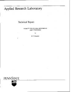
2. Model Details The model consists of a main program unit and several modules containing subroutines for describing both boundary conditions and various ecological, photochemical, and optical processes. The core subroutine functions are to: (1) define the spectral irradiant boundary conditions for visible and ultraviolet bands as a function of time-of-day, dayof-year, decimal latitude, and decimal longitude; (2) simulate the ecological element transformations; (3) simulate the attenuation of spectral, visible irradiance and perform the light-growth phytoplankton calculations; (4) simulate the attenuation of spectral, ultraviolet irradiance and compute the abiotic photochemical yields from CDOM; and (5) provide a solution to the simple one-dimensional case where state variables are subjected to vertical diffusion as the exclusive hydrodynamic process. This last step may be discarded when Neptune is integrated into more sophisticated hydrodynamic simulations. The main program unit is responsible for declaring and initializing the state variables and some key parameters that are sent to the optical and ecological subroutines. The main program unit then updates state variables after the ecological and photochemical changes are calculated and records the changes using netCDF format at user specified intervals. The number of state variables is flexible and is ultimately based on how many phytoplankton functional groups and classes of non-living organic matter are defined. For the initial Neptune start up, three size-based phytoplankton functional groups and three classes of non-living organic matter are defined. A size-based phytoplankton functional group approach was selected since both phytoplankton optical properties and phytoplankton affinity for nutrients may vary with gradations in overall cell size [Raven, 1998; Bricaud, et al., 2004]. With the exception of ammonium, nitrate (nitrite), inorganic phosphorus, and suspended sediments, the state variables are tracked in units of carbon concentration and the respective nitrogen and phosphorus contents are budgeted by using fixed C:N:P ratios. With the notable exception of heterotrophic bacteria, organic reservoirs become progressively carbon rich subsequent to the initial organic synthesis, i.e., phytoplankton primary production, such that excess nitrogen and phosphorus budgeted during organic matter transformations are returned to the ammonium and inorganic phosphorus reservoirs. Since heterotrophic bacteria are nitrogen and phosphorus enriched compared to their organic matter substrates, they may potentially require an inorganic nutrient supplement. This potential requirement is dependent upon the carbon gross growth efficiency (GGE) and the C:N:P ratio of the organic substrate. This calculation and its structural implications for the simulated ecosystem are discussed in Section 2.1. Figure 1 describes the base Neptune construct for state variables and material flow. Figure 2 shows the material pathways when terrestrial/estuarine boundary fluxes are included with additional state variables. The initial material flow is largely dependent upon the grazing fractions: carbon grazed by consumers is either respired or diverted to one of four non-living organic matter reservoirs. Figure 3 shows a potential structural modification that may describe colored dissolved organic carbon (CDOC) production as a consequence of bacterial processes.

Jolliff and Kindle

Page 5 of 49

Jolliff and Kindle

Page 6 of 49

} UV Photochemistry

Optical Submodels Spectral PAR - 400 - 700 nm Spectral UV 290 - 400 nm

Phytoplankton Gross Carbon (N, P) Assimilation f (nutrients, T, PAR)

:

Heterotrophic Inorganic P (N) Supplement

CDOC Colored Dissolved Organic Cabron; refractory humic substances, µM C

F5

Microphytoplankton 20 - 200 µm diamter µM C

Nanophytoplankton 2 - 20 µm diamter µM C

Picophytoplankton 0.2 - 2 µm diamter µM C

} Heterotrophic Bacteria µM C

Bacterial DOC Assimilation 30% efficiency

Bulk DOC Dissolved Organic Carbon; semilabile, colorless, µM C

F4

F2

Resp. Grazing Mortality

Small Particulate Detritus 0.2 - 10 µm, µM C

F1 - Respired C F2 - To Large Detritus F3 - To Small Detritus F4 - To Bulk DOC F5 - To CDOC

Detritus Solubilization Remin.

Large Particulate Detritus > 10 µm, µM C

F3

Carbon Fractions: the model assumes that grazing is the major carbon transformation pathway for primary production; picophytoplankton carbon is largely respired whereas proportionately more micophytoplankton carbon is transferred to detrital carbon pools.

Microbial Loop

Grazing Ivlev

Grazing Ivlev

Grazing Ivlev

F1

Figure 1. Neptune-1 material flow pathways: circles represent processes, rectangles represent state variables, and dashed lines are remineralization pathways.

Ammonium Nitrogen µM N

Nitrification

Nitrate Nitrogen µM N

Dissolved Inorganic Phosphorus µM P

DIC Dissolved Inorganic Carbon µM C

Basal Resp.

Jolliff and Kindle

Page 7 of 49

Boundary Flux

} UV Photochemistry



TCDOC Terrestrial/Fluvial flux of refractory humic substances, µM C


F5





Boundary Flux

:

} Boundary Flux

Heterotrophic Bacteria µM C

Bacterial DOC Assimilation 30% efficiency

Bulk DOC Dissolved Organic Carbon; semilabile, colorless, µM C

F4

F2



F1 - Respired C F2 - To Large Detritus F3 - To Small Detritus F4 - To Bulk DOC F5 - To CDOC

Detritus Solubilization Remin.


F3


Sediments

Microbial Loop

Grazing Ivlev

Grazing Ivlev

Grazing Ivlev

F1

Figure 2. Neptune-1 material flow pathways, as in Figure 1, with added terrestrial/fluvial/estuarine boundary fluxes.


Nitrification




Basal Resp.

Jolliff and Kindle

Page 8 of 49

} UV Photochemistry



:






F4

Bacterial Semilabile DOC Assimilation 30% efficiency

Bacterial Labile DOC Assimilation 30% efficiency

F2


Heterotrophic Bacteria µM C


F1 - Respired C F2 - To Large Detritus F3 - To Small Detritus F4 - To Labile DOC

Microbial Loop

} Detritus Solubilization Remin.


F3


Labile DOC Dissolved Organic Carbon; colorless, µM C

Semilabile DOC colorless, µM C

Grazing Ivlev

Grazing Ivlev

Grazing Ivlev

F1

Figure 3. Neptune-2 material flow pathways: circles represent processes, rectangles represent state variables, and dashed lines are remineralization pathways.


Nitrification




Basal Resp.

In the first construct (Figures 1 and 2), organic matter is implicitly produced as semilabile. The second (Figure 3) shows this process explicitly: DOC is produced at Redfield [1963] ratios and becomes carbon enriched through bacterial modification. This same process produces some CDOC. We show these two model structures as examples of potential modifications, though many more are possible. These will be referred to as Neptune-1 (Figure 1 and 2) and Neptune-2 (Figure 3). Below we describe the three main modeling components: ecological element cycling (2.1), the irradiant boundary condition and the visible optics that are coupled to the phytoplankton light-growth calculations (2.2), and the photochemical yield subroutine (2.3). The remaining section describes the hydrodynamics for the portable, onedimensional case that is coupled to the MODAS system (2.4). 2.1. Ecological Element Cycling The state equation for each state variable is given below, followed by a detailed description of the ecological computations. The main programming unit for describing element cycling and phytoplankton competition for nutrients is contained in the module poseidon.f90. The specific parameter symbols and values are given in Tables 1, 2, and 3. Parameter values are based on literature values [Holm and Armstrong, 1981; Ertel, et al., 1986; Fasham, et al., 1990; Benner, et al., 1992; Chisholm, 1992; Geider, 1992; Kemp, et al., 1993; Kirchman, 1994; Vallino, et al., 1996; Hopkinson, et al., 1998; Walsh, et al., 1999; del Giorgio and Cole, 2000; Kirchman, 2000; Mopper and Kieber, 2000; Carlson, 2002; Hopkinson, et al., 2002; Wozniak, et al., 2002; Lucea, et al., 2003; Paytan, et al., 2003], unless otherwise noted. Due to the large number of symbols and terms, supplemental tables that describe all symbols and acronyms may be found in the Appendix to aid the reader. In addition, a temperature field is required as input to the model since growth, grazing, and several other biological functions are temperature dependent. All phytoplankton carbon reservoirs (Pi; i = 1, 2, or 3 in Neptune Version 1), regardless of how many phytoplankton functional groups are established, conform to the general equation: ∂wph _ i Pi ∂Pi ∂P ∂ = −∇ • (VPi ) + Kz i + μnet _ i Pi − ∂t ∂z ∂z ∂z

(5)

where the first two terms on the right hand side (RHS) refer to the hydrodynamic components. The first term (RHS) is the advective flux divergence (in Cartesian coordinates), which is shown here for a generic tracer X: ⎛ ∂u ∂v ∂w ⎞ ∇ • (VX ) = ⎜ + + ⎟X ⎝ ∂x ∂y ∂z ⎠

Jolliff and Kindle

(6)

Page 9 of 49

Jolliff and Kindle

Page 10 of 49

calibrated to Q10 = 1.88 calibrated*3 [Vallino et al., 1996] [Holm and Armstrong, 1981]

0.063 oC-1 49.5 mmol C m-3 0.1 mmol N m-3 0.1 mmol P m-3

*1 – DOP/DOC ratios in marine environments are often 0 the model then switches to potential net gains of DIP from bacterial organic matter assimilation and respiration. DOC for Neptune-1 is produced via phytoplankton grazing, solubilization of particulate detritus, photobleaching of CDOC and is lost via heterotrophic bacterial assimilation/respiration: ∂DOC ⎡ 2 ⎤ ⎡ 3 ⎤ ⎡ 2 ⎤ ⎛g B⎞ = ⎢ ∑ CDOC ph _ i β i ⎥ + ⎢ ∑ m1_ iα 2 _ i Pi ⎥ + ⎢ ∑ Detiκ t (1 − X DET ) ⎥ − ⎜ rb ⎟ (42) ∂t ⎣ i =1 ⎦ ⎣ i =1 ⎦ ⎣ i =1 ⎦ ⎝ GGE ⎠ The first two terms on the RHS may be expanded or reduced. For Neptune-2, labile DOC is produced exclusively via phytoplankton grazing and is consumed by bacteria. ∂DOC1 ⎡ 3 ⎤ g B = ⎢ ∑ m1_ iα 2 _ i Pi ⎥ − rb X DOC (43) ∂t ⎣ i =1 ⎦ GGE The bacterial uptake of DOC1 not assimilated is transferred to both the CDOC and semilabile DOC pools, an additional parameter, XCDOC, is required to determine how this carbon is divided between the two potential receiving reservoirs. Semilabile DOC is thus produced as a consequence of bacterial modification of labile DOC, photobleaching of CDOC, and detrital solubilization. It may also be potentially consumed by the bacteria, if balanced growth requirements are met. ∂DOC2 ⎡ 2 ⎤ ⎡ 2 ⎤ ⎛ 1 ⎞ g B = ⎢ ∑ CDOC ph _ i β i ⎥ + ⎢ ∑ Detiκ t (1 − X DET ) ⎥ + g rb B(1 − X CDOC ) ⎜ − 1⎟ − rb (1 − X DOC ) ∂t ⎝ GGE ⎠ GGE ⎣ i =1 ⎦ ⎣ i =1 ⎦ (44)

Jolliff and Kindle

Page 19 of 49

Small organic carbon particulate detritus, SDET, is the sum of the phytoplankton production terms (via grazing) minus the solubilization and sinking: ∂w SDET ∂SDET ⎡ 3 ⎤ = ⎢ ∑ m1_ iα 3_ i Pi ⎥ − SDET κ t − d 1 ∂t ∂z ⎣ i =1 ⎦

(45)

as is large particulate detritus, LDET: ∂w LDET ∂LDET ⎡ 3 ⎤ = ⎢ ∑ m1_ iα 4 _ i Pi ⎥ − LDET κ t − d 2 ∂t ∂z ⎣ i =1 ⎦

(46)

The only significant difference between how large and small detritus are treated by the model is the rate of sinking. This is because ecological models that seek to mimic vertical carbon flux tend to assign high rates of sinking to large detrital particles [Walsh, et al., 1999], whereas much smaller particles that are still operationally defined as particulate (but sink much more slowly) are important for optical considerations. The detritus C:N:P ratio for both large and small detritus (DET) is initially fixed at 250:25:1 reflecting the nitrogen and phosphorus depletion of non-living particulate organic matter in coastal systems relative to Redfield ratios. Solubilization and remineralization of detritus are the two modeled loss pathways, both described by a decay rate maximum, κm, at 30oC, with the temperature dependence given by:

κ t = min[κ m , (κ m e Kt (T −30) )]

(47)

Remineralization of DET represents the implicit respiration of carbon by particle adhesive microbes. The biomass of particle adhesive microbes is not modeled explicitly, but their C:N:P ratios are assumed to be similar to water-column heterotrophic bacterioplankton--typically phosphorus rich relative to carbon (C:P ~ 53). The C:P ratio of DOC is not applicable here since it is assumed that DOP is preferentially remineralized from particles, as is often observed [Hopkinson, et al., 1997; Lucea, et al., 2003]. The C:P ratio of particle adhesive microbes determines the fraction of detrital organic carbon remineralized to DIC, XDET, by calculation of the required carbon assimilation for particle adhesive microbes: DET κ tξ3

ξ2

= DET κ t X DET , DET = SDET + LDET

(48)

The numerator on the left hand side of (48) is the total phosphorus fluxed out of the DET pool (detritus carbon times the rate of loss times the P:C ratio of detrital organic matter). The assumption is made that all of this phosphorus is used by microbes (the remineralization pathway), so if this term is multiplied by a bacterial C:P ratio (inverse of P:C for bacteria, ξ2) the total carbon flux to the remineralization pathway (an implicit overturn of the microbial population) is calculated. The expression may be rearranged

Jolliff and Kindle

Page 20 of 49

and simplified to the ratio of the bacteria C:P (53) to detritus C:P (250) determining the remineralized fraction (53:250 = 21%). Repeating the calculation for nitrogen with the remineralization fraction fixed at 21% but allowing for a labile DOC pool C:N ratio of 15 yields a particle adhesive microbe C:N ratio of 3.18, within the range of observation for marine bacteria [Kirchman, 2000]. Terrestrial boundary conditions serve as optional state variables. Terrestrial CDOC, terrestrial particulate organic detritus, and suspended lithogenic sediments are subjected to the same advection/diffusion as other state variables. The loss terms for suspended sediment is sinking and the terrestrial (or fluvial) CDOC is subjected to photochemical decay which is discussed in section 2.3. Organic detritus is subject to sinking and solubilization to semilabile DOC. Bulk changes is dissolved inorganic carbon (DIC) are budgeted, but the model does not presently compute the carbonate system (ΣDIC, alkalinity, pH) nor the potential air/sea gas exchange. Loss of DIC is budgeted as phytoplankton carbon assimilation and gains are a function of the respiratory, photochemical, and solubilization terms: ∂DIC ⎡ 3 ⎤ = ⎢ ∑ (m1_ iα1_ i + ε1_ i − g r _ i ) Pi ⎥ + B(m2 + ε 2 ) + DET κ t X DET + ∂t ⎣ i =1 ⎦ (49) 1 ⎡ 2 ⎤ g rb B( − 1) [ ( Neptune - 2 : (1- X DOC )] + ⎢ ∑ CDOC ph _ i (1 − βi ) ⎥ GGE ⎣ i =1 ⎦ The total system carbon, nitrogen, and phosphorus are checked to verify the system cycles elements conservatively. Finally, for phytoplankton functional groups where a maximum sinking speed is designated, the realized sinking rate is a function of the phytoplankton biomass. The concept is to simulate the formation of faster sinking cell aggregates at high biomass levels. This phenomenon is particularly pertinent to diatoms, or in our size-based approach, the microphytoplankton. We choose an expression that resembles the Michaelis-Menten uptake kinetics so that a half-saturation biomass constant, nw, can be designated, i.e., the biomass where the sinking rate is 50% of the maximum value: w phr _ i =

[ Pi ] w ph _ i (50) nw + [ Pi ]

This concludes the description and discussion of the core ecological element cycling computations contained within the module poseidon.f90. There are two fundamental quantities that must be calculated before the above changes may be computed: (1) the light-limited phytoplankton growth rate; and (2) the photochemical yields from CDOM. These quantities are computed in the optics module apollo.f90 and are explained in the following sections.

Jolliff and Kindle

Page 21 of 49

2.2. Bio-Optics and Photosynthesis The optical computations are coded in the FORTRAN 90 module apollo.f90, which contains the subroutines oceanblue (determines the visible light attenuation and lightcalculated phytoplankton carbon assimilation rates), and tcdoc (determines ultraviolet irradiance attenuation and the photochemical yields from CDOM). The subroutine angle in the module solar.f90 calculates the appropriate irradiance boundary condition and solar zenith angle as a function of position, day-of-year, and time-of-day. 2.2.1. Spectral Absorption Coefficients The additive nature of water column inherent optical properties (IOP’s) greatly simplifies their computation as a function of carbon reservoirs. For example, the total absorption coefficient may be expressed as the sum of individual constituents:

at(λ) = aw(λ) + acdm(λ) + aph(λ) (51) where the subscript w refers to pure seawater, cdm refers to colored detrital matter, which is the sum of the dissolved and particulate non-living organic matter absorption, and ph refers to all living phytoplankton absorption. All coefficients have units of inverse meters. Absorption of light by pure seawater is taken directly from published values [Pope and Fry, 1997]. Absorption by CDM is described by adding the total CDOC and the particulate detrital absorptions together:

⎡ NCDOC ⎤ ⎡ N DET ⎤ acdm (λ ) = ⎢ ∑ aCDOCi (λ ) ⎥ + ⎢ ∑ aDETi (λ ) ⎥ (52) ⎦ ⎣ i =1 ⎦ ⎣ i =1 The initial version requires the summation of marine CDOC and any potential terrestrial CDOC as well as the total number of particulate detrital pools. For the open ocean implementations, a minimum of 1 CDOC reservoir and 2 forms of particulate detritus are required. The conversion of the CDOC reservoirs to a spectral absorption value is dependent upon multiplication by the mass specific absorption, a*, parameterized for a reference wavelength (m2 mol-1; 440 nm). The spectral shape of the mass specific absorption values are determined by an exponential function that is dependent upon a spectral slope parameter, S: a *cdm (λ ) = a *cdm (440 nm) e (-S(λ -440)) (53)

For particulate detritus, as well as all particles besides living phytoplankton cells, the general methods described by [Stramski, et al., 2001], referred to hereafter as SBM 01, and the methods of [Mobley and Stramski, 1997], referred to hereafter as MS 97, are

Jolliff and Kindle

Page 22 of 49

Table 4. Particulate Absorption Parameters. Component

Absorption

units

ref.

Organic Carbon Detritus

σa,det (λ) = 8.791 X 10-4 exp(-0.00847 λ) μm2/particle

SBM 01

Mineral Sediment

σa,min (λ) = 1.013 X 10-3 exp(-0.00846 λ) μm2/particle

SBM 01

Heterotrophic Bacteria

σa,hbac (λ) = -6.0 X 10-18 (λ) + 5 X 10-15

m2/particle

MS 97

Detritus Carbon g C m-3 conversion to particles m-3 = 1.402 x 10-16 g C / particle (Calculated assuming a specific detritus scattering coefficient of 1.0 m2 g-1 and an organic SPM to organic carbon ratio of 2.6 = organic detritus carbon specific scattering 2.6 m2 g C-1 (555 nm), then back calculated using Stramski et al., 2001 expressions.) Mineral Sediment g m-3 conversion factor to particles m-3 = 3.23 X10-15 g / particle (Calculated assuming a mineral specific scattering coefficient of 0.5 m2 g-1 (555 nm), then back calculating using Stramski et al., 2001 expressions.) Bacteria moles nitrogen m-3 to bacteria particles per m-3 conversion factor = 2.94 X 10-14 mol N/particle (assuming 2.1 fg N per cell Lee and Furhman 1987)

Jolliff and Kindle

Page 23 of 49

Table 5. Backscattering Parameters Component

Backscatter

units

ref.

Organic Carbon Detritus σbb,det (λ) = 5.881 X 10-4 (λ)-0.8997

μm2/particle

SBM 01

Mineral Sediment

σbb,min (λ) = 1.790 X 10-2 (λ)-0.9140

μm2/particle

SBM 01

Heterotrophic Bacteria

σbb,hbac (λ) = 3.16 x 10-16 for all (λ)

m2/particle

MS 97

Picophytoplankton

σbb_phyt1 (λ) = 1.0 X 10-15 for all (λ)

m2/particle

SBM 01

Nanophytoplankton


m2/particle

SBM 01

Microphytoplankton


m2/particle

SBM 01

Detritus, Sediment, and Bacteria converted as in Table 4. Mass carbon m-3 to particle m-3 conversion for Picophytoplankton C:Chl ratio = 150.0 1.433 X 10-03 pg Chl per cell; Morel et al., 1993 Mass carbon m-3 to particle m-3 conversion for Nanophytoplankton C:Chl ratio = 100.0 1.433 X 10-03 pg Chl per cell; Bricaud et al., 1988 Mass carbon m-3 to particle m-3 conversion for Microphytoplankton C:Chl ratio = 50.0 1.433 X 10-03 pg Chl per cell; Ahn et al., 1992

Jolliff and Kindle

Page 24 of 49

utilized here to define particle absorption as the product of the particle concentration, Np (particles m-3), and the absorption cross-section per particle, σa(λ) (m2 per particle): ⎛ Nphbacσ a _ hbac (λ ) + Npdetσ a _ det (λ ) ⎞ ahbac (λ ) + adet (λ ) + ased (λ ) = ⎜ ⎟⎟ (54) ⎜ + Np σ sed a _ sed (λ ) ⎝ ⎠

where the subscript hbac refers to heterotrophic bacteria, det refers to particulate organic detritus, and sed refers to mineral-based suspended sediments. Table 4 describes the spectral relationships for the absorption cross-section per particle and the calculated mass concentration to particle density conversions, which are drawn from literature values [Lee and Fuhrman, 1987; Bricaud, et al., 1988; Ahn, et al., 1992; Morel, et al., 1993]. The absorption coefficient of living phytoplankton is calculated from the chlorophyll concentration. Two steps required for the computation are the assignment of the carbon to chlorophyll mass ratio, C:Chl, and the spectral chlorophyll-specific absorption coefficient a*(λ) (m2 mg-1). For the first step, a static C:Chl ratio is assigned to each phytoplankton functional group. For Neptune-1 and Neptune-2, the ratios are assigned at 150 for picophytoplankton, 100 for nanophytoplankton, and 50 for microphytoplankton. Once the chlorophyll reservoir of each phytoplankton functional group is computed, it is multiplied by the spectral chlorophyll-specific absorption term to compute the spectral absorption coefficients. Variability exists within the absorption per unit chlorophyll parameter due to phytoplankton taxonomic differences related to cell size and pigment composition [Cleveland, 1995; Bricaud, et al., 2004; Millan-Nunez, et al., 2004]. In general, however, both field and laboratory culture observations confirm that a* often decreases with increasing cell size. For the initial Neptune parameterization, picophytoplankton are given the highest a* values and microphytoplankton the lowest. The spectral values were adapted from Bricaud et al. [1995] (see their Table 2 and Figure 7). 2.2.2. Spectral Backscattering Coefficients Particles scatter as well as absorb incident irradiance. Estimating the total backscattering coefficient of the water column is essential to the approximation of visible light attenuation. The backscattering coefficient of pure seawater is assumed to be 50% of the total scattering coefficients across the visible spectrum (400 – 700 nm), which are taken from literature values [Smith and Baker, 1981; Pope and Fry, 1997]. CDOM backscattering is assumed to be negligible, leaving only particle backscattering as described by: bbp (λ ) = bbph (λ ) + bbhbac (λ ) + bbdet (λ ) + bbsed (λ ) (55)

Each backscattering coefficient may be described as the product of the particle concentration and the backscattering particle cross-section (m2 per particle):

Jolliff and Kindle

Page 25 of 49

⎛ Np phσ bb _ ph (λ ) + Nphbacσ bb _ hbac (λ ) + ⎞ bbp (λ ) = ⎜ ⎟⎟ (56) ⎜ Np σ λ σ λ ( ) + Np ( ) det bb _ det sed bb _ sed ⎝ ⎠

where ph refers to phytoplankton, and the remaining subscripts refer to heterotrophic bacteria, organic carbon detritus, and mineral-based suspended sediments, respectively. The expressions describing the value of each backscattering cross-section as a function of wavelength (nm) is proved in Table 5, as well as mass concentration to particle density conversion factors for the three classes of phytoplankton in Neptune-1 and Neptune-2. 2.2.3. Irradiant Boundary Condition Incident irradiance is modeled using the Gregg and Carder clear sky irradiance model [Gregg and Carder, 1990] for the visible range (400 – 700 nm), and equations adapted from the GCSOLAR UV model [Zepp and Cline, 1977] for the lower spectral range (290 - 400 nm). The models were combined into a single source code that gives direct and diffuse clear sky/band-centered irradiances just below the sea surface with Δλ = 10 nm for band-centered wavelengths 295 - 555 nm and Δλ = 20 nm for band-centered wavelengths 570 to 590 nm. A spectrally neutral reduction factor of 15% is applied to the direct and diffuse output to approximate the average reduction by clouds. Previous versions of this model [Jolliff, 2004] used National Center for Environmental Prediction’s (NCEP) reanalysis climatology cloud fractions to better estimate the impact of clouds. This technique can be implemented for any specific area where NCEP estimates are available. 2.2.4. Attenuation and the Visible Photon Budget The incident, planar, downwelling, and band-centered irradiance just below the air/sea interface, Ed(0-,λ; W m-2 nm-1) is first converted to the band-averaged photon flux (ρ, mol photons m-2 s-1):

ρ dir (λ ) = Ed _ dir (λ )

Δλ (nm) (57) q(λ )α

and

ρ diff (λ ) = Ed _ diff (λ )

Δλ (nm) (58) q (λ )α

where q (λ ) =

Jolliff and Kindle

hc (59) λ ( m)

Page 26 of 49

and h is Planck’s constant, c is the speed of light, and λ is wavelength in meters. The α in the RHS of equations (57) and (58) is Avogadro’s number and the wavelength bandwidth in these equations is in nanometers. The photon flux is then progressively attenuated over descending depth increments, Δz, by estimation of the downwelling attenuation coefficients for the direct and diffuse photon fluxes, Kd_dir(λ) and Kd_diff(λ), using the single-scattering approximation [Gordon, 1989]: K d _ dir ( z , λ ) =

at ( z , λ ) + bbt ( z , λ ) (60) θz

K d _ diff ( z , λ ) =

at ( z , λ ) + bbt ( z , λ ) (61) 0.7

and

where the direct attenuation is divided by the estimated direct path length, i.e., the cosine of the solar zenith angle, θz, once refracted through the air/sea interface. The diffuse attenuation is normalized by the cosine of a constant diffuse angle of ~45º. Attenuation over each discrete vertical depth interval is calculated following the BeerLambert Law: [ − K d _ dir ( z ,λ ) dz ]

ρ d _ dir ( z , λ ) = ρ d _ dir ( z − 1, λ )e

(62)

and [ − K d _ diff ( z , λ ) dz ]

ρ d _ diff ( z, λ ) = ρ d _ diff ( z − 1, λ )e

(63)

The total quantity of photons absorbed by the phytoplankton absorption fraction is retained over each depth level and used to calculate the light-limited growth rate and photoinhibition terms. Since backscattered photons may be potentially absorbed from the upwelling irradiance stream, some estimation of this contribution is required to better estimate the total absorbed photon budget. Photons absorbed from the upwelling irradiance stream are thus estimated by calculating the irradiance reflectance (R = Eu / Ed) for the discrete depth level [Mobley, 1994]: R( z, λ ) =

( K d ( z, λ ) − at ( z , λ ) μd −1 ) (64) ( K u ( z, λ ) + at ( z, λ ) μu −1 )

where the average cosine of upwelling irradiance, μu, is held constant at ~0.39 [Kirk, 1994]. The diffuse and direct notation was dropped for brevity; for the direct stream, μd =

Jolliff and Kindle

Page 27 of 49

θz, and for the diffuse stream μd = 0.7. Since the attenuation functions are approximated using the single scattering approximations, equation (64) may be recast as: R( z, λ ) =

bbt ( z , λ ) μd −1 (65) ⎡⎣ 2at ( z, λ ) + bbt ( z , λ ) ⎤⎦ μu −1

The upwelling stream for each depth interval is the downwelling flux multiplied by the irradiance reflectance. The important quantity towards which we are calculating is the photon flux absorbed by phytoplankton over each discrete depth increment, Δz. We begin by first tallying the downwelling photon flux density absorbed by phytoplankton, ρdv(z, λ), then calculating the upwelling analogue quantity, ρuv(z, λ):

(

ρ dv ( z , λ ) = Ω ⎡⎣ ρ d _ dir ( z − 1, λ ) − ρ d _ dir ( z , λ ) ⎤⎦ + ⎡⎣ ρ d _ diff ( z − 1, λ ) − ρ d _ diff ( z , λ ) ⎤⎦

) (66)

and Ω=

a ph ( z, λ )

1 (67) at ( z, λ ) + bbt ( z, λ ) Δz

Upwelling photons are also attenuated, although the upwelling irradiance increases with ascending depth. We thus approximate a discrete depth upwelling attenuation solely as a function of the depth-centered irradiance reflectance:

ρuv ( z, λ ) = Ω ( Rdif f ( z , λ ) ρ d _ diff ( z , λ ) + Rdir ( z, λ ) ρ d _ dir ( z , λ ) ) (1 − e[ − K

u ( z , λ ) Δz ]

) (68)

The spectrally integrated total photon flux harvest for phytoplankton, ρH (mol photons m-3 s-1) between grid levels z-1 and z is then the spectral summation of the calculations centered on depth level z: N

ρ H = ∑ ρuv ( z , Δλi ) +ρ dv ( z , Δλi ) (69) i =1

From first principles, only photons absorbed are available to do photochemical work. For the enzymatically mediated photochemical process of photosynthesis, this simple relationship can be expressed through the apparent quantum yield:

Φc = mole organic carbon produced / mole photons absorbed

(70)

The theoretical phytoplankton carbon yield (TCPY; mol carbon m-3 s-1) is then simply the calculated photon harvest multiplied by the apparent photosynthetic quantum yield: Jolliff and Kindle

Page 28 of 49

TPCY = ρ H ( ΦC ) (71) The maximum rate of photon absorption for the phytoplankton biomass (ρM; mol photons m-3 s-1) may then also be calculated as the product of the maximal temperatureadjusted rate of growth, the phytoplankton biomass, and the inverse of the quantum yield:

ρ M = g max T P (Φ c ) −1 (72) It follows that absorbed photon fluxes below this threshold would limit growth, while absorbed photon fluxes above this threshold may potentially inhibit growth. However, a strictly linear percentage reduction in maximal growth rate does not reproduce the normal hyperbolic relationship observed between growth (or photosynthetic rate) and irradiance (i.e., the PI curve). This is because photosynthesis is an enzymatically-mediated process, and the kinetics of such processes is best mimicked by Michealis-Menten-type functions. If the ratio of TPCY to the temperature-adjusted maximal assimilation rate (gmaxT) times the phytoplankton biomass (P) is less than unity, the light-limited growth calculation is performed:

gL =

Ψ ( g max T ) (73) MM ρ + Ψ

where Ψ=

TPCY (74) g max T P

and MMρ is the Michaelis-Menten half-saturation constant for photon flux, empirically determined to be ~ 0.072 for a wide variety of cultured phytoplankton [Rubio, et al., 2003]. If the TCPY ratio, Ψ, is greater than 4.0 then the estimated photoinhibitive effect on growth rate is estimated as a function of the incident photon flux [Rubio, et al., 2003]: gL =

1.0 1.0 + ⎡⎣ 20.0 ρ d λ ( z − 1) ⎤⎦

( g max T )

(75)

and N

ρ d λ ( z − 1) = ∑ ⎡⎣ ρ d _ dir ( z − 1, λi ) + ρ d _ diff ( z − 1, λi ) ⎤⎦ (76) i =1

Jolliff and Kindle

Page 29 of 49

These expressions mimic the photosynthesis-irradiance (PI) curve of marine phytoplankton, but are instead calculated as a function of the phytoplankton community’s maximal rate of growth, biomass, quantum yield of photosynthesis, and the absorbed photon flux. 2.3. Ultraviolet Attenuation and Photochemical Sub-Model. The attenuation of ultraviolet light and the computation of photochemical yields follow a construct similar to the one outlined in Section 2.2: the attenuation of photons with depth is budgeted such that the photon quantity absorbed by the reactive constituent is retained and multiplied by a quantum yield to determine the product yield over each discrete depth increment. The boundary visible irradiance values were calculated as a function of the solar zenith angle which was, in turn, calculated as a function of latitude, longitude, dayof-year, and time-of-day using equations set forth in Gegg and Carder [1990]. The expressions that describe incident downwelling ultraviolet irradiance as a function of the solar zenith angle were adapted from the GCSOLAR model version 1.2 (http://www.epa.gov/ceampubl/swater/gcsolar/) wherein the computations are based on the work of Baker et al. [1980]. The UV spectra are centered on the 295 – 395 nm bands at ∆λ=10 nm resolution. The stratospheric ozone amount must be designated before determining the UV boundary condition. Either a default value may be used or the UV boundary condition may be determined from Total Ozone Mapping Spectrometer global data (courtesy of NASA/GSFC; http://toms.gsfc.nasa.gov/ozone/ozoneother.html). For example, the grand mean of the zonal averages from each latitude band from the entire time series (1997 – 2005) was used determine the ozone value for the Gulf of Mexico and the Sargasso Sea. The first 11 spectral bandwidths of the irradiance boundary encompass the ultraviolet range 290 – 400 nm. The diffuse and direct components of the planar, downwelling, and band-centered irradiance just below the sea surface, Ed(0-,λ; W m-2 nm-1) are first converted to the band-averaged photon flux (ρ, mol photons m-2 s-1) following equations (57-59). We make the simplifying assumption that scattering within the ultraviolet (UV) range is negligible compared to absorption, such that the ultraviolet attenuation functions simplify to: K d _ dir ( z , λUV ) =

at ( z , λUV ) (77) θz

K d _ diff ( z , λUV ) =

at ( z , λUV ) (78) 0.7

and

Jolliff and Kindle

Page 30 of 49

where the direct attenuation is divided by the estimated direct path length, i.e., the cosine of the solar zenith angle, θz, once refracted through the air/sea interface. The diffuse attenuation is normalized by the cosine of a constant diffuse angle of ~45º. We further assume that CDM and water dominate the UV absorption:

at(λUV) ≅ aw(λUV) + acdm(λUV) (79) Absorption of light by pure seawater is taken directly from published values and absorption by CDM is described by adding the total CDOC and the particulate detrital absorptions together: ⎡N ⎤ ⎡N ⎤ acdm (λUV ) = ⎢ ∑ aCDOCi (λUV ) ⎥ + ⎢ ∑ aDETi (λUV ) ⎥ (80) ⎣ i =1 ⎦ ⎣ i =1 ⎦ Attenuation of the downwelling UV photon flux is calculated as in equations (62-63). No reflectance is considered since scattering is assumed to be negligible. The UV photon harvest for each discrete depth increment by CDOC component being considered is then described by: ⎛ ⎡ ρ d _ dir ( z − 1, λUV ) − ρ d _ dir ( z , λUV ) ⎤ + ⎞ ⎣ ⎦ ⎟ ⎜ ⎟ (81) ⎝ ⎡⎣ ρ d _ diff ( z − 1, λUV ) − ρ d _ diff ( z , λUV ) ⎤⎦ ⎠

ρ dv ( z, λUV ) = Ω ⎜

and Ω=

aCDM ( z , λUV ) 1 (82) at ( z , λUV ) Δz

The quantum yields for photochemical products from CDOM are adapted from Johannessen and Miller [2001] for the CO2 yield. They give a coastal value:

Φ ph _ CO2 (λ ) = e− (6.36+0.0140( λ − 290)) (83) and an open ocean value:

Φ ph _ CO2 (λ ) = e− (5.53+0.00914( λ − 290)) (84) which we apply to terrestrial CDOC and marine CDOC, respectively. We assume that the yield of CO2 from CDOM photochemical change is roughly equal to the yield of bleached DOC [Miller and Moran, 1997; Mopper and Kieber, 2000], such that the total loss of CDOM from photochemical change is double the spectrally integrated product yield of CO2:

Jolliff and Kindle

Page 31 of 49

11

total _ ph _ yield ( z ) = 2.0∑ ρ dv ( z ,λUVi )Φ ph _ CO2 (λUVi ) (85) i =1

Thus half of the total photochemical yield is diverted to the colorless, semilabile DOC pool and half returns to the DIC pool. Previous application of the photolysis sub-model [Jolliff, et al., 2003; Jolliff, 2004] suggested that CDOC likely consists of a photochemically reactive component and an inert, or background component. We thus modify the total absorption description to accommodate a background absorption CDM signal, aCDMb, that is not linked to any state variable carbon reservoir:

at(λUV) ≅ aw(λUV) + acdm(λUV) + acdmb(λUV) (86) where the background signal is a constant 0.015 m-1 at 440 nm, and is spectrally described by equation (53) using a spectral slope, S, of 0.015. Application of this formulation to the Sargasso Sea suggests the background signal is closer to 0.006 m-1 at 440 nm. Discerning ways to represent photochemically active and inert chromophores in the model remains an active area of research and development. 2.4. MODAS-Derived Vertical Diffusivity for the One-Dimensional Case For the one-dimensional application of the model, the eddy mixing coefficients, Kz(z), may be inferred from the Modular Ocean Data Assimilation System vertical temperature fields without any additional information. To accomplish this task, we adapt the vertical mixing parameterization scheme of Pacanowski and Philanderer [1981], or PP81 for brevity. Their scheme solves for Kz(z) as a function of the local gradient Richardson number:

Kz ( z ) =

v0 + κ b (87) (1 + αRi g ) n +1

where v0 = 100 cm2 s-1, κb, the background diffusivity, is 0.1 cm2 s-1, and the empirical constants are assigned the PP81 values of n = 2, and α = 5. As in Li et al. [2001], the local Richardson gradient, Rig, is calculated as the ratio of the Brunt-Väisälä frequency to the vertical current shear. The Brunt-Väisälä frequency is calculated from the temperature-based density gradients (assuming a constant salinity) from solution of the UNESCO equation of state. Since the vertical current shear is unknown, we backcalculated a bulk shear approximation by assuming the vertical eddy diffusivity at depths above the isothermal layer depth are ~100 cm2 s-1. The isothermal layer depth is defined as the first descending depth below 10-meters where the temperature difference from 10meters depth exceeds 0.8 deg C [Kara, et al., 2000]. The mean Brunt-Väisälä within the isothermal layer depth divided by the maximal diffusivity yielded a bulk shear term that was used to calculate eddy diffusivities below the isothermal layer depth using the PP81 scheme.

Jolliff and Kindle

Page 32 of 49

2.5. Model Integration The flow of the code execution is shown in Figure 4. The main program unit declares/initializes the state variables, and then opens/reads boundary conditions and hydrodynamic/temperature files necessary for code execution. The irradiant boundary condition is computed ahead of code execution for a range of solar zenith angles, and then selected during code execution depending upon position and time. The photochemical yield calculations (Section 2.3) and light-limited growth calculations (Section 2.2) are computed first and the necessary information (light-limited growth rate, photochemical yields) is passed to the element cycling subroutine (Section 2.1). The hydrodynamic advection/diffusion and particle sinking computations are performed and then the code loops to another time-step execution. The state variables as well as some optical information are recorded at the end of each daily iteration. For the one-dimensional application, the MODAS script to generate temperature fields and the FORTRAN code to generate eddy diffusion coefficients must be run ahead of model execution. Presently, we are combining 5-years or more of daily MODAS fields into a composite climatology for a given area of interest. The MODAS script, the eddy diffusion and temperature climatology, and the main program unit must all generate the same grid dimensions and resolution. The latitude and longitude location must also be specified in the main program unit in order to correctly calculate the sun angle as a function of time and location.

Jolliff and Kindle

Page 33 of 49

(Boxmodel.f90) - Main Program Unit use - NETCDF, cdfmodule - netCDF output use - types_dec - variable types declarations use - solar - sun angle calculations use - apollo - optical calculations (2.2-2.3) use - mixmaster - 1-D hydrodynamics use - sinker - sinking subroutine use poseidon - element cycling (2.1) parameter declarationsd variable declarations grid defieniitons (space, time)

Open output file and define output variables

Output netCDF file

Open and read irradiance files: (direct, diffuse, spectral dim., sun angle dimension)

Irradiacne Output File

Make climatology Solve for Density Richardson # Impute Kz

Open and read hydrodynamic variables; eddy diffusivity for 1-D case, and Temperature

Hydrodynamics (Kz, T)

Initial Conditions Define Threshold Values (if needed)

Optional Initialization File

vismaker.f90 290 - 700 nm specify ozone specify sun angles

Daily T Files

MODAS script define depth grid location; generate synthetic Temperature files

Continued

Figure 4. Model code execution flow chart.

Jolliff and Kindle

Page 34 of 49

Begin Day Loop1 Assign Daily Temp, Kz

Begin Timestep Loop2 (360 or 1800 s) Call Angle determine irradiant boundary

solar.f90

Y Light?

Call TCDOC Call oceanblue

apollo.f90

photochemical yields = (X) light-limited growth = (X) N photochemical yields = (0) light-limited growth = (0)

Call ecomaker (element cycling)

poseidon.f90

Call adv/diff.

mixmaster.f90

Call Sinking

sinker.f90

L1?

Update State Equations Remin. bottom grid -optional

Write to output file

L2?

END

Figure 4. Continued, Model code execution flow chart.

Jolliff and Kindle

Page 35 of 49

3. Example Application: Western Gulf of Mexico Briefly, we provide an example of our application of Neptune to the western Gulf of Mexico. The MODAS script was used to generate daily temperature fields for five years from 1 to 161-meters depth at 1-meter resolution. These data were merged into a single annual climatology (Figure 5) and the eddy diffusion coefficients were estimated from this field. The nutrient fields (NO3, NH4, DIP) were initialized using temperature to nutrient relationships observed in the northeastern Gulf of Mexico [Jochens, et al., 2002]. The model was then run towards a steady state solution: the annual cycle was repeated for five years and the system was forced to element conservation by implicitly remineralizing particulate detritus within the lower-most grid cell. Our detailed model description of the relationship between carbon reservoirs and optical properties allowed us to compare the steady state model solution with Sea-viewing WideField-of-view Sensor (SeaWiFS) mean climatology extracted from a 1º x 1º area surrounding our location of interest. Both the standard OC4v4 chlorophyll algorithm and the QAA algorithms [Lee, et al., 2002] were applied to the extracted SeaWiFS data so that model/satellite comparisons of surface phytoplankton absorption (443 nm), surface chlorophyll concentration, and CDM absorption (412 nm) could be made (Figure 6). The model mimics both the amplitude and phase of the satellite signals. We were able to use the satellite data to begin to constrain model structure and model parameter selection, as described elsewhere [Jolliff, et al., 2006]. The model also reproduced the depth distribution of chlorophyll common to stratified waters, i.e., the appearance of the deep chlorophyll maximum, particularly during summer months (Figure 7). An interesting result of our model is that the DOC and CDOC distributions are out of phase (Figure 8). In fact, DOC apparently accumulates in surface waters during summer whereas CDOC is depleted during this time. This type of CDOC to DOC decoupling has been observed in subtropical oceans [Nelson, et al., 1998; Steinberg, et al., 2004]. Our continuing sensitivity analyses further demonstrate that the cycling of DOC impacts the recycling of nutrients and, in turn, the amplitude and phase of the seasonal surface chlorophyll signal. We are now investigating these model features using in situ data from the Sargasso Sea. The portability of the combined Neptune/MODAS modeling construct allows us to examine how data may constrain the model in any region around the globe where data are available. We also plan to couple refined versions of Neptune to regional applications of the Naval Research Laboratory Coastal Ocean Model so as to apply our methods of satellite validation and constraints to three-dimensional fields.

Jolliff and Kindle

Page 36 of 49

(A)

MODAS Temperature (B)

depth (m)

oC

Month

Figure 5. (A) Map of western Gulf of Mexico test area for Neptune, and (B) the 5-year annual MODAS climatology for one-dimensional temperature profiles.

Jolliff and Kindle

Page 37 of 49

(Α)

(Β)

SeaWiFS phytoplankton abs. (m-1; 443 nm) Model phytoplankton abs.

SeaWiFS chl-a (mg m-3) Model chl-a

(C)

SeaWiFS CDM absorption (m-1; 412 nm) Model CDM absorption

Figure 6. The model’s surface results are compared to the mean annual cycle (2 years are shown) as estimated from daily averages of SeaWiFS data (2002 - 2004) of phytoplankton absorption (A), surface chlorophyll concentration (B), and CDM absorption (C). The satellite data suggest that the relationship between chlorophyll-a and phytoplankton absorption is not constant; phytoplankton absorption efficiency per unit chlorophyll-a (a* m2 mg-1 pigment) decreases during the winter. The model mimics this pattern via changes in the phytoplankton composition: during winter, microphytoplankton are more abundant. Microphytoplankton are parameterized with a lower a* than picophytoplankton. Picophytoplankton Chl-a

Nanophytoplankton Chl-a

Microphytoplankton Chl-a

Figure 7. The model simulates the transitions between the winter/spring well-mixed chl-a distribution and the summer stratified water column wherein a deep chlorophyll maximum is evident. Simulated surface waters during summer are dominated by the picophytoplankton size class. DOC (no color) µM C

Colored DOC µM C

Heterotrophic Bacterial Biomass µM C

depth (m)

Figure 8. The model also shows opposite trends for colorless, bulk dissolved organic carbon (DOC) and colored dissolved organic carbon (CDOC) distributions: DOC accumulates in surface waters during summer whereas surface water CDOC is depleted during this time. Accumulated DOC is eventually broken down by a heterotrophic bacterial biomass that peaks during late summer, early fall.

Jolliff and Kindle

Page 38 of 49

4. Summary A modeling system has been constructed that combines ecological element cycling, photochemical processes, and bio-optical processes into a single simulation that may be coupled to hydrodynamic models that provide temperature fields as well as the advection/diffusion of state variables. The model is derived from a history of ocean biogeochemical models that describe the transformation of elemental reservoirs (carbon, nitrogen, phosphorus) based upon lower trophic-order ecosystem function. Here we relate these reservoirs to optical properties in order to describe how the spectrally decomposed attenuation of both visible and ultraviolet irradiance stimulates photochemical and photosynthetic changes in upper ocean elemental reservoirs. For our initial model startup, we have parameterized phytoplankton functional groups based on size since size appears to impact both nutrient affinity and optical property variability in consistent ways. Our model description of the relationship between reservoirs of organic carbon and optical properties allows us to use satellite ocean color data to begin to validate and constrain the model. We have thus far coupled the model to the Modular Ocean Data Assimilation System, which permits us to examine the one-dimensional case in any region of interest around the globe. This portability will further allow us to continue to refine and constrain the model using satellite ocean color data as well as in situ data, wherever it becomes available.

Jolliff and Kindle

Page 39 of 49

Appendix. Comprehensive List of Symbols and Acronyms Table A1. Ecological Symbols and Acronyms Ks n nw μnet gr gL gN gP gmaxT gm30 μnetb grb gCb gNb gPb gmaxTb gm30b ε1 ε2 ε1m ε2m m1 m2 m1max m2max m1maxT m2maxT b κt κm X XDOC XDET XCDOC MBNA BNR MBPA BPR DOC CDOC T Kt

Jolliff and Kindle

general form of the Michaelis-Menten half-saturation constant model Michaelis-Menten (MM) half-saturation constants (see parameters list) half-saturation constant for phytoplankton sinking; mmol C m-3 net community carbon assimilation rate for phytoplankton; s-1 maximal realized gross carbon ass’n rate; s-1 light-limited maximal gross carbon ass’n rate; s-1 nitrogen-limited maximal gross carbon ass’n rate; s-1 phosphorus-limited maximal gross carbon ass’n rate; s-1 temperature adjusted gross maximal carbon ass’n rate; s-1 maximum gross carbon ass’n rate at 30º C; s-1 net community carbon ass’n rate for heterotrophic bacteria; s-1 maximal realized net cellular carbon ass’n het. bacteria; s-1 maximal carbon-limited bacteria net cellular carbon ass’n; s-1 maximal nitrogen-limited bacteria net cellular carbon ass’n; s-1 maximal phosphorus-limited bacteria net cellular carbon ass’n; s-1 temperature-adjusted gross cellular maximal carbon assimilation rate; s-1 maximum gross cellular carbon assimilation rate; s-1 temperature-adjusted phytoplankton basal respiration rate; s-1 temperature-adjusted bacterial basal respiration rate; s-1 maximum phytoplankton basal respiration rate at 30º C; s-1 maximum bacterial basal respiration rate at 30º C; s-1 realized phytoplankton mortality rate (grazing); s-1 realized heterotrophic bacteria mortality rate (grazing); s-1 phytoplankton mortality rate (grazing) at 30º C; s-1 heterotrophic bacteria mortality rate (grazing) at 30º C; s-1 temperature-adjusted phytoplankton mortality rate (grazing); s-1 temperature-adjusted heterotrophic bacteria mortality rate (grazing); s-1 Nitrate uptake inhibition term Temperature-adjusted particulate organic detritus solubilization rate; s-1 Maximum particulate organic detritus solubilization rate at 30º C; s-1 Nitrate to total nitrogen uptake fraction Fraction of Bacterial DOC uptake from Labile DOC Fraction of solubilized DET remineralized Fraction of labile carbon transferred to CDOC pool (Neptune-2) Maximum potential Bacterial Nitrogen Assimilation; mmol N m-3 Bacterial Nitrogen Requirement; mmol N m-3 Maximum potential Bacterial Phosphorus Assimilation; mmol P m-3 Bacterial Phosphorus Requirement; mmol P m-3 Dissolved Organic Carbon; mmol C m-3 Colored Dissolved Organic Carbon; mmol C m-3 Temperature; º C Temperature inhibition coefficient

Page 40 of 49

Nr Iv α

θ ξ

GGE B P NO3 NH4 DIP Nitro DET LDET SDET wd1 wd2 wd3 wph wphr β Vm t

Maximum nitrification rate at 30º C; s-1 Ivlev grazing attenuation parameter; m3 (mmol C)-1 Grazing transformation fractions (see parameters list) Molar N:C ratio (see parameters list) Molar N:P ratio (see parameters list) Heterotrophic Bacteria Gross Carbon Growth Efficiency Heterotrophic Bacteria Carbon; mmol C m-3 Phytoplankton Carbon; mmol C m-3 Nitrogen as nitrate (+nitrite); mmol N m-3 Nitrogen as ammonium; mmol N m-3 Dissolved Inorganic Phosphate (largely as orthophosphate); mmol P m-3 Quantity of NH4+ to NO3 conversion per unit time; mmol N m-3 s-1 particulate organic detrital carbon; the sum of LDET and SDET; mmol C m-3 large particulate organic detrital carbon; mmol C m-3 small particulate organic detrital carbon; mmol C m-3 Sinking velocity small particulate organic detritus; m s-1 Sinking velocity large particulate organic detritus; m s-1 Sinking velocity of suspended mineral sediments; m s-1 Maximum sinking velocity of phytoplankton; m s-1 Realized maximum sinking velocity of phytoplankton; m s-1 Fraction of photochemical CDOC yield as bleached DOC Maximum uptake rate for ideal Michaelis-Menten kintetics time; seconds

Table A2. Optical Symbols and Acronyms λ α h c ρ(λ) ρd_dir(λ) ρd_diff(λ) ρdv(λ) ρuv(λ) ρH ρM ρdλ Ed (λ) Eu (λ) q bb(λ)

Jolliff and Kindle

wavelength; nanometers unless otherwise specified Avogadro’s number Planck’s Constant speed of light; m s-1 photon flux; mol photon m-2 s-1 downwelling, direct photon flux; mol photon m-2 s-1 downwelling, diffuse photon flux; mol photon m-2 s-1 downwelling photon flux density; mol photon m-3 s-1 upwelling photon flux density; mol photon m-3 s-1 spectrally integrated photon flux density absorbed (harvested) by phytoplankton; mol photon m-3 s-1 maximum potential (saturating) phytoplankton absorbed photon flux density; mol photon m-3 s-1 spectrally integrated sum of direct and diffuse incident photon fluxes; mol photon m-2 s-1 band-centered downwelling planar irradiance W m-2 nm-1 band-centered upwelling planar irradiance W m-2 nm-1 Energy; Joules spectral backscattering coefficient; m-1

Page 41 of 49

a(λ) a*(λ) a*chl(λ) a*cdm(λ) Φ ΦC Φph Φph_CO2 (λ) θz Np σbb(λ) σa(λ) TCPY Ψ

μd μu

MMp Kd_dir(λ) Kd_diff (λ) Ku(λ) R(λ) z Ω

spectral absorption coefficient; m-1 spectral mass specific absorption; m-1 (mass units)-1 chlorophyll-specific absorption; m2 mg-1 cdm mass specific absorption; m2 mol-1 apparent quantum yield; mol product yield per mol photon absorbed apparent quantum yield for photosynthesis; mol carbon assimilated per mol photons absorbed apparent quantum yield for CDOC photochemistry; mol CDOC altered per mol photons absorbed spectral apparent quantum yield for CDOC photochemistry specific to CO2 yield; mol CO2 per mol photons absorbed Cosine of the refracted solar zenith angle particle concentration; particles m-3 backscattering particle cross-section (m2 particle-1) absorption particle cross-section (m2 particle-1) Theoretical Photosynthetic Carbon Yield, the product of the absorbed photon flux density and the apparent quantum yield of photosynthesis; mol carbon m-3 s-1 ratio of TCPY to maximum temperature-adjusted carbon growth yield cosine of the average downwelling irradiance angle cosine of the average upwelling irradiance angle Michaelis-Menten half-saturation constant for photon saturation Attenuation function for downwelling irradiance, direct component; m-1 Attenuation function for downwelling irradiance, diffuse component; m-1 Attenuation function for upwelling irradiance; m-1 Irradiance reflectance depth level; -meters absorption fraction per depth increment (as defined in the text); m-1

Table A3. Optical Subscripts sed – mineral suspended sediments det – particulate organic detritus cdm – colored detrital matter cdmb – background cdm signal cdom – colored dissolved organic matter ph – phytoplankton p – particulates dir – direct component of the spectral irradiance diff – the diffuse component of the spectral irradiance

Jolliff and Kindle

Page 42 of 49

Acknowledgements: This research is a contribution to the Naval Research Laboratory 6.1 project, “Coupled Bio-Optical and Physical Processes in the Coastal Zone” under program element 61153N sponsored by the Office of Naval Research, Dr. John Kindle, Principal Investigator. This research was supported by the National Research Council’s Post-Doctoral Research Associateship Program, and partially supported by the Office of Naval Research, grant number N0001405WX20735. Paul Martinolich provided assistance with SeaWiFS data processing; C. N. Barron and C. Rowley provided assistance with the MODAS system. Literature Ahn, Y.-W., A. Bricaud, and A. Morel (1992), Light backscattering efficiency and related properties of some phytoplankters, Deep-Sea Research, 39, 1835-1855. Baker, K., R. Smith, and A. E. S. Green (1980), Middle ultraviolet radiation reaching the ocean surface, Journal of Photochemistry and Photobiology B: Biology, 32, 367-374. Balch, W. M., K. A. Kilpatrick, and C. C. Trees (1996), The 1991 coccolithophore bloom in the central North Atlantic. 1. Optical properties and factors affecting their distribution, Limnology and Oceanography, 41, 1669 - 1683. Benner, R., J. D. Pakulski, M. McCarthy, J. I. Hedges, and P. G. Hatcher (1992), Bulk Chemical characteristics of dissolved organic matter in the ocean, Science, 255, 15611564. Bricaud, A., A. Bedhomme, and A. Morel (1988), Optical properties of diverse phytoplankton species: experimental results and theoretical interpretation, Journal of Plankton Research, 10, 851-873. Bricaud, A., H. Claustre, J. Ras, and K. Oubelkheir (2004), Natural Variability of phytoplankton absorption in oceanic waters: Influence of the size structure of algal populations, Journal of Geophysical Research, 109, doi:10.1029/2004JC002419. Bricaud, A., A. Morel, M. Babin, K. Allali, and H. Claustre (1998), Variations of light absorption by suspended particles with chlorophyll a concentration in oceanic (case 1) waters: Analysis and implications for bio-optical models, Journal of Geophysical Research, 103, 31033-31044. Carder, K. L., and R. G. Steward (1985), A remote-sensing reflectance model of a red tide dinoflagellate off west Florida, Limnology and Oceanography, 30, 286-298. Carder, K. L., R. G. Steward, G. R. Harvey, and P. B. Ortner (1989), Marine humic and fulvic acids: their affects on remote sensing of ocean chlorophyll, Limnology and Oceanography, 34, 68-81.

Jolliff and Kindle

Page 43 of 49

Carlson, C. A. (2002), Production and Removal Processes, in Biogeochemistry of Marine Dissolved Organic Matter, edited by D. A. Hansell and C. A. Carlson, pp. 91-151, Elsevier Science. Chisholm, S. W. (1992), Phytoplankton size, in Primary Productivity and Biogeochemical Cycles in the Sea, edited by P. G. Falkowski and A. D. Woodhead, pp. 213-237, Plenum. Cleveland, J. S. (1995), Regional models for phytoplankton absorption as a function of chlorophyll-a concentration, Journal of Geophysical Research, 100, 13333 - 13344. Cullen, J. J. (1990), On models of growth and photosynthesis in phytoplankton, Deep-Sea Research, 37, 667-683. del Giorgio, P. A., and J. J. Cole (2000), Bacterial Energetics and Growth Efficiency, in Microbial Ecology of the Oceans, edited by D. L. Kirchman, pp. 289-325, Wiley-Liss, Inc. Ertel, J. R., J. I. Hedges, A. H. Devol, J. E. Richey, and M. Ribeiro (1986), Dissloved humic substances in the Amazon river system, Limnology and Oceanography, 31. Fasham, M. J. R., H. W. Ducklow, and S. M. McKelvie (1990), A nitrogen based model of plankton dynamics in the oceanic mixed layer, Journal of Marine Research, 48, 591639. Geider, R. J. (1992), Respiration: Taxation without Representation? edited by P. Falkowski and A. D. Woodhead, pp. 333-360, Plenum Press, Primary Productivity and Biogeochemical Cycles in the Sea. Gordon, H. R. (1989), Dependence of the diffuse reflectance of natural waters on the sun angle, Limnology and Oceanography, 34, 1484-1489. Gregg, W., and J. J. Walsh (1992), Simulation of the 1979 spring bloom in the MidAtlantic Bight: A coupled physical/biological/optical model, Journal of Geophysical Research, 97, 5723-5743. Gregg, W. W., and K. L. Carder (1990), A simple spectral solar irradiance model for cloudless maritime atmospheres, Limnology and Oceanography, 35, 1657-1675. Holm, N. P., and D. E. Armstrong (1981), Role of nutrient limitation and competition in controlling the populations of Asterionella formosa and Microcystis aeruginosa in semicontinuous culture, Limnology and Oceanography, 26, 622-634. Hopkinson, C. S., I. Buffam, J. Hobbie, J. Vallino, M. Perdue, B. Eversmeyer, F. Prahl, J. Covert, R. Hodson, M. A. Moran, E. Smith, J. Baross, B. Crump, S. Findlay, and K. Foreman (1998), Terrestrial inputs of organic matter to coastal ecosystems: An intercomparison of chemical characteristics and bioavailability, Biogeochemistry, 43, 211-234.

Jolliff and Kindle

Page 44 of 49

Hopkinson, C. S., B. Fry, and A. L. Nolin (1997), Stoichiometry of dissolved organic matter dynamics on the continental shelf of the northeastern U.S.A., Continental Shelf Research, 17, 473-489. Hopkinson, J., Charles S., J. J. Vallino, and A. Nolin (2002), Decomposition of dissolved organic matter from the continental margin, Deep Sea Research Part II: Topical Studies in Oceanography, 49, 4461-4478. Ivlev, V. S. (1955), Experimental Ecology of the Feeding of Fishes, 302 pp., Pischepromizdat, Moscow. Jamart, B. M., D. F. Winter, and K. Banse (1979), Sensitivity analysis of a mathematical model of phytoplankton growth and nutrient distribution in the Pacific Ocean in the northwestern U.S. coast, Journal of Plankton Research, 1, 267-290. Jochens, A. E., S. F. DiMarco, W. D. Nowlin, Jr., R. O. Reid, and M. C. Kennicutt II (2002), Northeastern Gulf of Mexico Chemical Oceanography and Hydrography Study: Synthesis Report, 586 pp, U.S. Department of the Interior, Minerals Management Service, Gulf of Mexico OCS Region, New Orleans, Louisiana. Johannessen, S. C., and W. L. Miller (2001), Quantum yield for the photochemical production of dissolved inorganic carbon in seawater, Marine Chemistry, 76, 271-283. Jolliff, J. K. (2004), The Influence of Coastal Effluent and Deep Water Masses on surface Optical Properties and Margin Productivity in the Northeastern Gulf of Mexico: A ThreeDimensional Simulation Analysis, Doctoral Dissertation thesis, 153 pp., University of South Florida, Tampa, Florida. Jolliff, J. K., B. Penta, and J. C. Kindle (2006), Ecosystem Analysis from Space: Diagnosis of Phytoplankton Functional Groups from Satellite Data and Skill Assessment for Coupled Hydrodynamic-Ecosystem Models, Eos Trans. AGU, 87(52), Fall Meet. Suppl., Abstract OS43A-0637. Jolliff, J. K., J. J. Walsh, R. He, R. H. Weisberg, A. Stovall-Leonard, P. G. Coble, R. Conmy, C. Heil, B. Nababan, H. Zhang, C. Hu, and F. E. Muller-Karger (2003), Dispersal of the Suwannee River plume over the West Florida shelf: Simulation and observation of the optical and biochemical consequences of a flushing event, Geophysical Research Letters, Vol. 30, No. 13, 1709, doi:10.1029/2003GL016964. Kara, A. B., P. A. Rochford, and H. E. Hurlburt (2000), Mixed layer depth variability and barrier layer formation over the North Pacific Ocean, Journal of Geophysical Research, 105, 16783-16801. Kemp, P., S. Lee, and J. LaRoche (1993), Estimating the growth rate of slowly growing marine bacteria from RNA content, Appl. Environ. Microbiol., 59, 2594-2601. Kieber, D. J., J. McDaniel, and K. Mopper (1989), Photochemical source of biological substrates in sea water: implications for carbon cycling, Nature, 637-639. Jolliff and Kindle

Page 45 of 49

Kirchman, D. L. (1994), The uptake of inroganic nutrients by heterotrophic bacteria, Microbial Ecology, 284, 255-271. Kirchman, D. L. (2000), Uptake and regeneration of inorganic nutrients by marine heterotrophic bacteria, in Microbial Ecology of the Oceans, edited by D. L. Kirchman, pp. 261-289, John Wiley and Sons, Inc. Kirk, J. T. O. (1994), Light and Photosynthesis in Aquatic Ecosystems, 509 pp., Cambridge University Press, Cambridge. Lee, S., and J. A. Fuhrman (1987), Relationships between biovolume and biomass of naturally derived marine bacterioplankton, Appl. Environ. Microbiol., 53, 1298-1303. Lee, Z., K. L. Carder, and R. A. Arnone (2002), Deriving inherent optical properties from water color: a multiband quasi-analytic algorithm for optically deep waters, Applied Optics, 41, 5755-5772. Lee, Z., and C. Hu (2006), Global distribution of Case-1 waters: An analysis from SeaWiFS measurements, Remote Sensing of Environment, 101, 270-276. Li, X., Y. Chao, J. C. McWilliams, and L.-L. Fu (2001), A comparison of two verticalmixing schemes in a Pacific Ocean general circulation model, Journal of Climate, 14, 1377-1398. Lucea, A., C. M. Duarte, S. Agusti, and M. Sondergaard (2003), Nutrient (N, P and Si) and carbon partitioning in the stratified NW Mediterranean, Journal of Sea Research, 49, 157-170. Michaelis, L., and M. L. Menten (1913), Die kinetik der invertinwirkung, Biochem. Z., 49, 333-369. Millan-Nunez, E., M. E. Sieracki, R. Millan-Nunez, J. R. Lara-Lara, G. Gaxiola-Castro, and C. C. Trees (2004), Specific absorption coefficient and phytoplankton biomass in the southern region of the California Current, Deep-Sea Research II, 51, 817-826. Miller, W. L., and M. A. Moran (1997), Interaction of photochemical and microbial processes in the degradation of refractory dissolved organic matter from a coastal marine environment, Limnology and Oceanography, 42, 1317-1324. Mobley, C. D. (1994), Light and Water, 595 pp., Academic Press, San Diego, CA. Mobley, C. D., and D. Stramski (1997), Effects of microbial particles on oceanic optics: methodology for radiative transfer modeling and example simulations, Limnology and Oceanography, 42, 550-560. Mopper, K., and D. J. Kieber (2000), Marine photochemistry and its impact on carbon cycling, in The effects of UV radiation in the marine environment, edited by S. De Mora, et al., pp. 101-129, Cambridge University Press, Cambridge, United Kingdom.

Jolliff and Kindle

Page 46 of 49

Mopper, K., Z. Xianliang, R. J. Keiber, D. J. Keiber, R. J. Sikorski, and R. D. Jones (1991), Photochemical degradation of dissolved organic carbon and its impact on the oceanic carbon cycle, Nature, 353, 60-62. Moran, M. A., and R. G. Zepp (1997), Role of photoreactions in the formation of biologically labile compounds from dissolved organic matter, Limnology and Oceanography, 42, 1307-1316. Morel, A. (1988), Optical modeling of the upper ocean in relation to its biogenous matter content (case I waters), Journal of Geophysical Research, 93, 10749-10768. Morel, A., Y.-W. Ahn, F. Partensky, D. Vaulot, and H. Claustre (1993), Prochlorococcus and Synechococcus: a comparative study of their size, pigmentation and related optical properties, Journal of Marine Research, 51, 617-649. Morel, A., and L. Prieur (1977), Analysis of variation in ocean color, Limnology and Oceanography, 22, 709-722. Nelson, N. B., D. A. Siegel, and A. F. Micheals (1998), Seasonal dynamics of colored dissolved material in the Sargasso Sea, Deep-Sea Research I, 45, 931-957. Pacanowski, R. C., and S. G. H. Philander (1981), Parameterization of Vertical Mixing in Numerical Models of the Tropical Oceans, Journal of Physical Oceanography, 11, 14431451. Paytan, A., B. J. Cade-Menun, K. McLaughlin, and K. L. Faul (2003), Selective phosphorus regeneration of sinking marine particles: evidence from 31P-NMR, Marine Chemistry, 82, 55-70. Pope, R. M., and E. S. Fry (1997), Absorption spectrum (380-700nm) of pure water: II. Integrating cavity measurements, Applied Optics, 36, 8710-8723. Raven, J. A. (1998), The twelfth Tansley Lecture. Small is beautiful: the picophytoplankton, Functional Ecology, 12, 503-513. Redfield, A. C., B. H. Ketchum, and F. A. Richards (1963), The influence of organisms on the composition of seawater, in The Sea, Volume 2, edited, pp. 26-77, Interscience, New York, New York. Rubio, C. F., F. G. Camancho, J. M. Fernandez Sevilla, Y. Chisti, and E. M. Grima (2003), A mechanistic model of photosynthesis in microalgae, Biotechnology and Bioengineering, 81, 459-473. Sarmiento, J. L., R. D. Slater, M. J. R. Fasham, H. W. Ducklow, J. R. Toggweiler, and G. T. Evans (1993), A seasonal three-dimensional ecosystem model of nitrogen cycling in the North Atlantic euphotic zone, Global Biogeochemical Cycles, 7, 417-450.

Jolliff and Kindle

Page 47 of 49

Sathyendranath, S., L. Watts, E. Devred, T. Platt, C. Caverhill, and H. Maass (2004), Discrimination of diatoms from other phytoplankton using ocean-colour data, Marine Ecology Progress Series, 272, 59-68. Siegel, D. A., S. Maritorena, N. B. Nelson, and M. J. Behrenfeld (2005), Independence and interdependencies among global ocean color properties: Reassesssing the bio-optical assumption, Journal of Geophysical Research, 110, C0701, doi:10.1029/2004JC002527. Siegel, D. A., S. Maritorena, N. B. Nelson, D. A. Hansell, and M. Lorenzi-Kayser (2002), Global distribution and dynamics of colored dissolved and detrital organic materials, Journal of Geophysical Research, 107, 3228, doi:3210.1029/2001JC000965. Smith, R. C., and K. S. Baker (1981), Optical properties of the clearest natural waters (200-800 nm), Applied Optics, 20, 177-184. Spitz, Y. H., J. R. Moisan, and M. R. Abbott (2001), Configuring an ecosystem model using data from the Bermuda Atlantic Time Series, Deep-Sea Research II, 48, 17331768. Steinberg, D. K., N. B. Nelson, C. A. Carlson, and A. C. Prusak (2004), Production of chromophoric dissolved organic matter (CDOM) in the open ocean by zooplankton and the colonial cyanobacterium Trichodesmium spp., Marine Ecology Progress Series, 267, 45-56. Stramski, D., A. Bricaud, and A. Morel (2001), Modeling the inherent optical properties of the ocean based on the detailed composition of the planktonic community, Applied Optics, 40, 2929-2945. Vallino, J., C. S. Hopkinson, and J. E. Hobbie (1996), Modeling bacterial utilization of dissolved organic matter: Optimization replaces Monod growth kinetics, Limnology and Oceanography, 41, 1591-1609. Walsh, J. J. (1975), A spatial simulation model of the Peru upwelling ecosystem, DeepSea Research, 22, 201-236. Walsh, J. J., D. A. Dieterle, F. E. Muller-Karger, R. Bohrer, W. P. Bissett, R. J. Varela, R. Aparicio, R. Diaz, R. Thunell, G. T. Taylor, M. I. Scranton, K. A. Fanning, and E. Peltzer (1999), Simulation of carbon-nitrogen cycling during the spring upwelling in the Cariaco Basin, Journal of Geophysical Research, 104, 7807-7825. Walsh, J. J., T. E. Whitledge, F. W. Barvenik, C. D. Wirick, S. O. Howe, W. E. Esaias, and J. T. Scott (1978), Wind events and food chain dynamics within the New York Bight, Limnology and Oceanography, 23, 659-683. Westbury, T. K., D. A. Siegel, and A. Subramaniam (2005), An improvised bio-optical model for the remote sensing of Trichodesmium spp. blooms, Journal of Geophysical Research, 110, C06012, doi:10.1029/2004JC002517.

Jolliff and Kindle

Page 48 of 49

Wozniak, B., J. Derza, D. Ficek, and R. Majchrowski (2002), Dependence of the photosynthesis quantum yield in the oceans on environmental factors, Oceanologia, 44, 439-459. Wroblewski, J. S. (1977), A model of phytoplankton plume formation during variable Oregon upwelling, Journal of Marine Research, 35, 357-394. Zepp, R. G., and D. M. Cline (1977), Rates of Direct Photolysis in Aquatic Environments, Environmental Science and Technology, 11, 359-366.

Jolliff and Kindle

Page 49 of 49