NBER WORKING PAPER SERIES IS UNIVERSAL HEALTH ... - Core

NBER WORKING PAPER SERIES

IS UNIVERSAL HEALTH CARE IN BRAZIL REALLY UNIVERSAL? Guido Cataife Charles J. Courtemanche Working Paper 17069 http://www.nber.org/papers/w17069

NATIONAL BUREAU OF ECONOMIC RESEARCH 1050 Massachusetts Avenue Cambridge, MA 02138 May 2011

We thank Jose Fernandez, Joe Terza and seminar participants at ICF International and University of California San Diego for valuable comments and suggestions. There exists no conflict of interest related to this research. The views expressed herein are those of the authors and do not necessarily reflect the views of the National Bureau of Economic Research. NBER working papers are circulated for discussion and comment purposes. They have not been peerreviewed or been subject to the review by the NBER Board of Directors that accompanies official NBER publications. © 2011 by Guido Cataife and Charles J. Courtemanche. All rights reserved. Short sections of text, not to exceed two paragraphs, may be quoted without explicit permission provided that full credit, including © notice, is given to the source.

Is Universal Health Care in Brazil Really Universal? Guido Cataife and Charles J. Courtemanche NBER Working Paper No. 17069 May 2011 JEL No. I0,O12 ABSTRACT Since Brazil's adoption of a universal health care policy in 1988, the country's health care has been delivered by a mix of private providers and free public providers. We examine whether income-based disparities in medical care usage still exist after the development of the public network using a nationally representative sample of over 46,000 Brazilians from 2003. We find robust evidence of a positive association between income and doctor visits, private doctor visits, and private medical expenditures. Interestingly, we also find a pro-rich disparity in public doctor visits that disappears after including local area fixed effects to account for variation in availability and quality of medical services across localities. We then estimate the income elasticity of private medical expenditures to be well below one, suggesting that private care remains a necessity despite the availability of free public care. These results suggest that the public health care system in Brazil is not effectively reaching the segments of the population that need it most.

Guido Cataife ICF International 3 Corporate Square NE Suite 370 Atlanta, GA 30329 [email protected] Charles J. Courtemanche Bryan School of Business and Economics University of North Carolina at Greensboro P. O. Box 26170 Greensboro, NC 27402 and NBER [email protected]

1

Introduction and Background In 1988, Brazil adopted a universal health care policy that created a network of public

providers to deliver a full range of health services free of charge. Subsequently, the government expanded the public network and created the Family Health Program (Programa Saúde da Família; PSF), which assigns a team composed of a doctor, a nurse, a nurse’s assistant and several health workers to provide free health care to all families in a particular area. This paper presents evidence that signi…cant income-based disparities in health care utilization – in both the private and public sectors –exist in Brazil despite the country’s commitment to universal health care. We also estimate the income elasticity of private medical expenditures and conclude that private sector care remains a necessity. Brazil’s health care system consists of both public and private sub-systems. The public system –called sistema único de saúde (SUS) –was created and de…ned in the Federal Constitution of 1988 and the 1990 Organic Health Law. Three main principles of universality, integrality, and decentralization guide the system. Universality means that health care is a universal right; it is the state’s duty to provide health care to all citizens free of charge. Integrality means that public health assistance must comprise primary, secondary, and tertiary levels of care. Decentralization means that the management and organization of health services is the responsibility of the municipalities. Brazil is the …fth largest country in the world in both land area and population, and the SUS is one of the world’s largest public health care systems. Its ambulatory system consists of 56,640 units and assists 350 million cases annually, while 6,493 hospitals and 487,058 hospital beds are part of the SUS network. In 2001, the SUS conducted 250 million consultations, 200 million laboratory tests, and 70 million high complexity procedures (Rehem de Souza, 2002).1 The SUS network consists of a mix of public, non-pro…t, and for-pro…t providers, but all services are paid by the federal, state, and municipal governments (Uga and Santos, 1

High complexity procedures include tomography, magnetic resonance imaging, hemodialysis, and chemotherapy sessions.

2

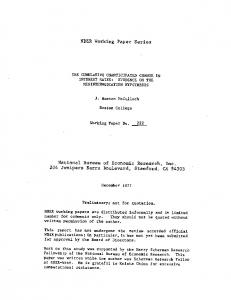
2007). The private health care system –called sistema suplementar de saúde (SSS) –comprises those private institutions that do not belong to the SUS. Patients are responsible for their own medical bills in the private system. Individual and group health insurance plans are available to help defray the costs, but coverage rates are low.2 Though only 20% of the population participates in the SSS, it accounts for approximately half of the country’s medical expenditures. Brazil exhibits striking geographic variation in both health and access to health care. The infant mortality rate of 35.5 per 1,000 in the Northeast –the country’s least economically developed region –is more than double the rate of 15.6 per 1,000 in the country’s most developed region the Southeast. Endemic and transmittable diseases are notoriously persistent in the less developed North, Northeast and Center-West regions (Pan American Health Organization, 2008). In some states, more than 50% of all registered deaths are attributed to uncertain causes, potentially re‡ecting a lack of health care services (Lobato, 2000). Access to SUS hospitals varies widely between municipalities. Wherever the population is highly concentrated (typically wealthier areas), several hospitals are present and the average distance from households to their closest establishment is short. Where population groups are scattered along a extensive territory (typically poorer areas), hospitals are scarce and obtaining care usually requires traveling long distances. Figure 1 illustrates this discrepancy by showing the distribution of hospitals a¢ liated with the SUS network in the northeastern state of Bahia.3 Despite their large land area, most municipalities in the northwestern area 2

There are four types of health insurance plans: self-managed health plans, prepaid group practice plans, medical cooperative plans, and health insurance company plans. Self-managed health plans o¤er services for the employees of a given …rm. Prepaid group practice plans (17 million enrollees) o¤er di¤erent services, depending on the contract signed. The services may be through a network of facilities and professionals or free choice with reimbursement. Medical cooperative plans (10 million enrollees) are similar to prepaid group practices but the health services are strictly from a network of facilities and professionals. Health insurance company plans (6 million enrollees) consist of free choice of professionals and facilities combined with reimbursement to the user (Lobato, 2000). 3 Bahia is fourth and …fth among Brazilian states in terms of population and territory, respectively. Its economy represents a 5% of Brazil’s total GDP, which makes it the richest state in the northeastern region (http://www.sidra.ibge.gov.br).

3

of the state have 6 or fewer hospitals, while much smaller municipalities in the eastern area of the state have 16 or more hospitals. These geographic di¤erences highlight the need for empirical research to examine whether Brazil’s public health care network is adequately reaching those in need. As a whole, the literature to date suggests that universal health care coverage in Brazil has improved health but that the extent of public sector provision remains insu¢ cient. Macinko et al. (2006 and 2007), Rasella et al. (2010), and Morsch et al. (2001) documented a negative association between PSF coverage and infant or …ve-year mortality rates. However, in a study of health expenditure that also includes dental care and medicines, Xu et al. (2003) found that Brazil had the second-highest prevalence of catastrophic medical expenditures out of 59 countries despite the availability of free public care. Rodriguez et al. (2009) found that less than half of elderly individuals with chronic conditions had a medical visit in the preceding six months. Using a sample of elderly individuals from southern Brazil, Bos (2007) estimated a positive relationship between the number of public outpatient clinics in a municipality and residents’ probability of using the public system. Goldbaum et al. (2005) compared two areas of São Paulo City and found that disparities in health care utilization on the bases of income and education were more evident in the area that was not covered by the PSF. Barros and Bertoldi (2008) examined a sample of 869 households and found that the proportion of income spent on private health services was similar across economic groups. In a study of the northeastern state of Ceará, where PSF covers practically the whole population, Maciel et al. (2010) show that the need of physicians to have multiple jobs is a major obstacle to SUS e¢ cacy. We contribute to this growing literature in three ways.4 First, to our knowledge we are the …rst to use a large nationally representative sample to test for income-based disparities in health care utilization in Brazil. Second, we examine whether these disparities are purely 4

More broadly, we contribute to the extensive literatures on disparities in health care utilization and the income elasticity of health care. See Wagsta¤ and Van Doorslaer (2000), Goddard and Smith (2001), and Rannan-Eliya and Somanathan (2006) for reviews of the former. See Gerdtham and Jonsson (2000) and Getzen (2000) for reviews of the latter.

4

driven by di¤erences in the private sector or whether disparities exist in the free public sector as well. Third, we compute an estimate of the income elasticity of private sector medical expenditures in Brazil, which provides an objetive measure of whether private health care is a luxury or necessity. We estimate a positive relationship between income and doctor visits, private doctor visits, and private medical expenditures that persists even after including demographic, health, living condition, and religion controls as well as state or local area …xed e¤ects. Interestingly, we also …nd evidence of a positive association between income and public doctor visits that persists after adding the control variables but becomes negative when we include local area …xed e¤ects. This is consistent with the pro-rich disparity in public sector utilization being driven by di¤erences in medical care access and quality between rich and poor areas. Additionally, we estimate the income elasticity of private medical expenditures of well below one, so private care remains a necessity in Brazil despite the availability of free public care. Together, these results suggest that the public health care system in Brazil is not e¤ectively reaching everyone. More broadly, our …ndings underscore the di¢ culty of implementing a universal health care system in a country with an extensive geographic territory.

2

Data We use the publicly available 2003 Pesquisa de Orçamentos Familiares (POF; Survey of

Family Budget), a nationally representative dataset of 48,470 households collected by the Brazilian Institute of Geography and Statistics. The survey contains detailed information on all types of income and expenditure in a one year period, as well as socioeconomic and demographic characteristics of the household members. Health expenditures are divided into two broad categories: pharmacy and health care access. Our analysis focuses on the latter, and more speci…cally expenditures on medical visits. For each medical visit, the survey

5

speci…es the type of doctor, amount spent, payment method, and type of provision. Type of provision includes public sector, health insurance company (HIC), or private agent other than a HIC.5 Table 1 provides summary statistics for the income and medical variables. Table 2 presents summary statistics for the demographic, health, living condition, and religion variables used as controls in our analysis. After dropping observations with missing data, our sample consists of 46,720 observations. In 46% of households, at least one member visited a doctor at least once in the reference year. 37.2% of households made at least one visit to a public doctor, while only 13% of households made at least one visit to a private doctor. Only 20.6% of households had a member enrolled in a private health insurance plan. Among those households who spent money on private medical care, the average expenditure was R$68.1, or 4.5% of household income. Figure 2 illustrates the relationship between household income and overall, private, and public doctor visits, estimated nonparametrically. Figure 3 plots the relationship between income and expenditures on private care.6 As expected, both graphs show a positive association between income and private sector utilization that persists throughout the income distribution. A more surprising …nding is the positive association between income and public sector utilization that persists until approximately the mean household income of R$1,516. Also noteworthy is the overall low level of utilization, particularly for the poor. The poorest households make only 0.4 doctor visits per year; for an average-sized household of 4 members, this equates to only 0.1 visits per year per individual. Even households at the high end of the income distribution only make approximately 1 doctor visit per year, or 0.25 per individual. These observations provide preliminary evidence that Brazil’s universal health care system is not e¤ectively reaching everyone. We next turn to regression analysis for a 5

Private agents other than a HIC typically refer to physicians established in particular consultories charging a ‡at fee per visit. By "private" we therefore mean paid care in the SSS, as opposed to free care at the private institutions that participate in the SUS. 6 Neither …gure excludes households with no doctor visits/medical expenditures. For ease of viewing, we exclude the top 1% of the income distribution from the …gures.

6

more thorough investigation.

3

Doctor Visits

3.1

Models

We begin by analyzing the relationship between household income and the number of doctor visits – overall, private, and public – by household members. All three dependent variables have a signi…cant number of zeros, and the process governing the transition from non-participation to the …rst doctor visit is likely systematically di¤erent than the process governing successive doctor visits after a household is already participating in the health care system. We therefore utilize two-part hurdle models where the …rst part predicts participation and the second part predicts number of visits conditional on participation. For the …rst part, we estimate the associations between income and probability of overall, public, and private participation using a linear probability model. We avoid probit and logit models because some speci…cations will include almost 4,000 local area …xed e¤ects, and probit and logistic …xed e¤ects estimators have been shown to su¤er from a sizeable amount of bias – even with the number of observations per group as large as it is in our dataset – because of the incidental parameters problem (Kalb‡eisch and Sprott, 1970; Hsiao, 1996; Greene, 2004). While the linear probability model has the drawback of predicting outside of the 0-1 range, its coe¢ cient estimates are reliable (Angrist, 2001), and the purpose of our analysis is to accurately estimate average e¤ects of the covariates rather than predict outcomes.7 The regression equation is

P (visits > 0jincome; X) =

7

0

+

1

ln(income) + X0

(1)

Accordingly, for the models without local area …xed e¤ects the linear probability model estimates for the income coe¢ cient are virtually identical to the marginal e¤ects from probit and logistic regressions. The probit and logit results are available upon request.

7

where visits is the number of either overall, public, or private doctor visits, income is household income, and X is a vector of control variables. We take the log of income because of the skewness of the income distribution. This also gives the coe¢ cient for income a straightforward interpretation: the approximate percentage point e¤ect on doctor visits of a 100% increase in income. We compute heteroskedasticity-robust standard errors that allow for clustering within each of the 3,984 local geographic areas de…ned by the POF.8 The second part of the model estimates the relationships between the covariates and the number of overall, public, and private doctor visits among those who cleared the participation "hurdle" in the …rst step. Since the dependent variables are counts, we estimate zerotruncated Poisson models of the form

E[visitsjincome; X; visits > 0] =

exp( 0 + 1 ln(income) + X0 ) 1 P (visits = 0jincome; X)

(2)

where the sample is restricted to participators.9 In unreported regressions we also considered truncated negative binomial models and found that the coe¢ cient estimate and standard error for

1

were virtually identical to the truncated poisson in all cases. Since the coe¢ cient

estimates are di¢ cult to interpret, we also compute the marginal e¤ect of ln(income) on visits among participators, which we de…ne as

1.

Combining the results from the two parts allows us to approximate the overall marginal e¤ect of ln(income) on visits for the whole sample, conditional on X, as follows: dE[visits] = d ln(income)

1

visitsjvisits > 0 +

1

(P [visits > 0])

(3)

where visitsjvisits > 0 is the mean number of visits among participators (1.73, 1.25, and

8

The POF’s local geographic areas are de…ned speci…cally for the survey and do not correspond exactly to more commonly-used geographic units. Brazil consists of 5,560 municipalities, so the POF’s geographic areas are on average slightly larger than a municipality (Pan American Health Organization, 2008). 9 See Greene (2007; p. 37-38) for a derivation of this model. Though the poisson …xed e¤ects model is estimated with maximum likelihood, Greene (2004) notes that it is not susceptible to the incidental parameters problem.

8

1.71 for overall, private, and public) and P [visits > 0] is the sample participation rate (0.46, 0.13, and 0.37 for overall, private, and public). We use several di¤erent variations of the vector of controls X, starting with a regression with no controls in which X = ? and then gradually incorporating groups of variables. We begin by adding a set of demographic characteristics consisting of the gender, age, education, race, and family size variables from Table 2. Since household doctor visits are directly related to household size, we model family size ‡exibly with a set of dummy variables.10 A common challenge in identifying the ceteris paribus relationship between income and health care utilization is controlling for systematic di¤erences in health status between socioeconomic groups. The next two sets of covariates address this issue. First is a set of health variables that includes the underweight, overweight, and obesity indicators from Table 2 as well as the health insurance indicator from Table 1. Since the POF does not contain more detailed health information, we also add an extensive set of controls for living conditions consisting of number of rooms in the family’s home plus the indicators for dwelling type, water source, toilet type, electricity, and ‡oor type. While these living condition variables are not speci…cally health variables, they should capture many (although obviously not all) of the mechanisms through which a low socioeconomic status would adversely a¤ect health. We next add the religion variables to proxy for cultural di¤erences that might impact medical care usage. Our last two models include …xed e¤ects – …rst for each of the 27 states and then for each of the 3,984 local geographic areas.11 Given the substantial within-state variation in SUS network accessibility shown in Figure 1, the area-level …xed e¤ects are vital to capturing di¤erences in physician supply.

10

Speci…cally, we include a dummy variable for whether the family size is 1, another for 2, another for 3, etc. Since few households have 10 or more members, we combine these households together into one category. 11 We do not use the POF sampling weights since some of the Stata modules used in the analysis do not support them. In unreported regressions (available upon request), we veri…ed that the results from the regressions for which sampling weights are supported are not sensitive to their use.

9

3.2

Results

Tables 3-5 present the results for number of overall, private, and public doctor visits, respectively. Panel A of each table reports the coe¢ cient estimates and standard errors for the income variable from the linear probability models (equation (1)), while Panel B gives the marginal e¤ects and standard errors for the income variable from the zero-truncated poisson regressions (equation (2)). Column (1) represents the simple regression with ln(income) as the only explanatory variable. The remaining columns gradually add the sets of controls, building up to the state and local area …xed e¤ects models in columns (6) and (7). In column (8), we estimate the full area …xed e¤ects model excluding the 15% of households in which at least one member has private health insurance, thereby restricting the sample to those who would face the full cost of private care. To conserve space, we do not report the full regression output for the control variables but instead present F statistics from tests of the joint statistical signi…cance of the variables in each group. We begin the discussion with the results for overall number of doctor visits (sum of private and public) from Table 3. The coe¢ cient for ln(income) is positive and statistically signi…cant at the 0.1% level in all speci…cations for both participation and number of visits conditional on participation. In Panel A, the coe¢ cient estimate for ln(income) is generally stable across columns (1)-(6) and implies that a 100% increase in income raises P (visits > 0) by 3.3-4.6 percentage points. Adding local area …xed e¤ects in columns (7)-(8) reduces the magnitude to 2.1-2.4 percentage points. In Panel B, a 100% increase in income is associated with an additional 0.28 doctor visits among participators in the regression with no controls. Adding the demographic and living condition controls attenuate this relationship somewhat, and the e¤ect stabilizes at 0.12-0.13 visits across columns (3)-(6). Including the local area …xed e¤ects in columns (7)-(8) reduces the e¤ect further, to 0.05-0.06. The overall marginal e¤ect across the entire population –shown in the last row of the table –ranges from 0.110.13 visits after controlling for the demographic, health, and living condition covariates but shrinks to 0.06-0.07 visits after adding the local area …xed e¤ects. To summarize, the 10

evidence points to a pro-rich disparity in overall doctor visits that operates somewhat, but not completely, through community-speci…c factors such as the availability of physician services. Table 4 turns to the results for private doctor visits. Ln(income) is again statistically signi…cant at the 0.1% level in all speci…cations for both private participation and number of private visits conditional on private participation. In Panel A, after adding the demographic controls the coe¢ cient estimate for income stabilizes and implies that a 100% increase in income is associated with a 4.7-5.6 percentage point increase in the probability a household member visited a private network doctor. Panel B shows that a 100% increase in income is associated with 0.09-0.22 more private visits among those households that participate in the private medical care sector. The estimates of the overall marginal e¤ect suggest that a 100% increase in income leads to 0.07-0.10 more private doctor visits per household across the population. In contrast to Table 3, the local area …xed e¤ects do not mitigate the relationship between income and visits (in fact, they strengthen this relationship among private sector participators), so the pro-rich disparity in private visits does not operate through community-speci…c factors. Table 5 presents the results for public doctor visits. Importantly, despite the fact that public sector medical care is free, there is still a positive association between income and number of public doctor visits across columns (1)-(6). This relationship operates through an increase in the frequency of public visits among those who participate in the public sector (Panel B), rather than through increasing the probability of participation in the public sector (Panel A). A 100% increase in income increases the number of public doctor visits by participators by 0.30 in the regression with no controls. The demographic and health controls attenuate this relationship somewhat, and the estimates stabilize at 0.11-0.14 visits across columns (3)-(6). This translates to a population-wide marginal e¤ect of 0.04-0.06. Interestingly, the pro-rich disparity in public visits switches to a pro-poor disparity after the local area …xed e¤ects are added. In columns (7) and (8), a 100% increase in income reduces the probability of public sector participation by 1.6-1.7 percentage points and has

11

no statistically detectable e¤ect on number of doctor visits among participators, leading to an overall marginal e¤ect of -0.02 to -0.03. Our …nding of a positive relationship between income and public visits that turns negative after accounting for local area …xed e¤ects is consistent with the pro-rich disparity being driven by the relative scarcity of public health clinics in poor, sparsely-populated areas, or by the quality of public care being lower in these areas. Once the …xed e¤ects control for these community-level attributes, the estimates appear to re‡ect only a substitution from the less luxurious public network to the more luxurious private network as income increases. At …rst glance, the results could also …t with a demand-side explanation in which rich and poor areas di¤er systematically in their demand for health. However, if demand-side factors were driving the results then we would also expect to see the positive e¤ect of income on private doctor visits disappear after adding local area …xed e¤ects, which – as discussed with the results from Table 4 – is not the case. Multicollinearity is another conceivable explanation, as adding detailed location controls could potentially eliminate too much of the variation in income to obtain accurate estimates of its e¤ect. The evidence, however, seems to strongly rule out this possibility. First, there is no loss in precision when area …xed e¤ects are added. Second, the variance in‡ation factor (VIF) for income in the local area …xed e¤ects regression is only 3, well below the typically-accepted level of 10 at which the extent of multicollinearity is considered to be problematic (Wooldridge, 2006:99).12 Third, if multicollinearity in the income variable was a problem in an analysis of public visits then it should also be a problem with private visits, but Table (4) showed that adding area …xed e¤ects made almost no di¤erence in the estimated income e¤ect on private visits.13 To summarize, Tables 3-5 present two pieces of evidence that the network of free public health care providers is not e¤ectively reaching everyone in Brazil. First, private doctor 12

V IF = 1=(1 Rj2 ), where Rj2 is the R2 from a linear regression of ln(income) on the control variables plus the local area …xed e¤ects. 13 Another conceivable explanation for the positive relationship between income and public doctor visits is if the "free" public clinics charge patients an informal fee –e¤ectively a bribe –in order to be seen. While there is evidence of such behavior in some developing countries (Ensor and Thompson, 2006), we are not aware of any anecdotal or empirical evidence that these practices are common in Brazil.

12

visits are a necessity instead of a luxury. Second, there is a positive relationship between income and public sector utilization that persists through the addition of the individual-level controls but disappears when area …xed e¤ects –which capture local factors such as number of public clinics –are added.

4

Private Medical Expenditures

4.1

Models

We next turn to an analysis of the relationship between income and total household outof-pocket expenditures on private medical care. This analysis also requires dealing with a cluster of observations with zero expenditure. In the medical expenditures literature, there is controversy over whether Heckman’s sample selection model or the two-part model is the most appropriate when potential expenditure is the main outcome of interest (see Madden, 2008 and Jones, 2000). However, our main outcome of interest is actual expenditure –the expenses Brazilians actually spent on health care, rather the expenses they would spend had they sought health care. Dow and Norton (2003) underscore that the appropriate model in this case is the two-part model as no selection bias is actually present in the sample.14 We therefore estimate the e¤ect of income on medical expenditures using the following two-part model:

P [y > 0jincome; X] =

0

+

E[ln(y)jy > 0; income; X] =

0

1

+

ln(income) + X0

1

(4)

2

ln(income) + X0

2

(5)

where y is out-of-pocket household medical expenses while income and X again represent household income and the vector of controls. We again estimate a linear probability model 14

Sometimes this is referred as the "true zeros" case in the literature, since a zero expenditure observation represents no consumption, and not an unobserved value.

13

in the …rst part (equation (4)) to avoid the incidental parameters problem; in unreported regressions (available upon request) we veri…ed that the marginal e¤ects in the …rst part are virtually identical using probit or logit models. We estimate the second part (equation (5)) with ordinary least squares (OLS) using the 8,024 observations with y > 0. By combining the results from the two parts we can compute the marginal e¤ect of ln(income) on the expectation of ln(y), conditional on X, for the whole sample as follows: dE [ln(y)] = d ln(income)

1

ln(y)jy > 0 +

1

(P [y > 0])

(6)

where P [y > 0] is the proportion of the sample with non-zero expenditures, which is 0.17, and ln(y)jy > 0 is the mean log of expenditures among participators, which is 5.48. This derivative can be interpreted as the approximate income elasticity of medical expenditures at the mean.15 As with doctor visits, we estimate the model …rst with no control variables and then gradually build up to the area …xed e¤ects speci…cation. We again also estimate the area …xed e¤ects model dropping those households where at least one individual has health insurance, which restricts the sample to those for whom all expenditures are out-of-pocket costs.

4.2

Results

Table 6 reports the results. Panel A presents the results from the participation equation (4), while panel B presents the results from the expenditure equation (5). The last row of the table combines the estimates from Panels A and B to obtain the income elasticity. In all speci…cations, we …nd a positive and statistically signi…cant relationship between income and both probability of paticipation and expenditures conditional on participation. In Panel A, the …rst three sets of control variables attenuate the relationship between income 15

In unreported regressions we veri…ed that our estimated elasticities are very similar to the coe¢ cient estimates from a log-log model with the full sample. (In order to estimate a log-log model with the full sample, we add 1 to y so than ln(y) is de…ned even for those with no medical expenditures.)

14

and participation somewhat, but from columns (4)-(8) the estimate stabilizes at 0.051-0.056. A 100% increase in income therefore increases the probability of participation in the private sector by approximately 5.1 to 5.6 percentage points. Panel B shows that after the living condition controls are added in column (4) the estimated relationship between ln(income) and y among those with non-zero expenditures ranges from 0.15-0.19. Combining the results from Panels A and B yields estimated income elasticities that are consistently well below 1. After the living condition controls are added in column (4), the elasticity remains within the 0.32-0.33 range regardless of whether additional controls or …xed e¤ects are included or those with health insurance are dropped from the sample. Private medical spending is therefore a necessity instead of a luxury, providing further evidence to support the hypothesis that individuals living in poor (generally remote) areas spend money on private care because of a lack of access or quality in the public sector.

5

Disparities and the Family Health Program We close our empirical analysis by examining whether income-based disparities in health

care utilization are systematically di¤erent in states with higher rates of Family Health Program (PSF) coverage.16 The Brazilian government created the PSF in 1994 in an e¤ort to improve primary health care access and reduce service inequality. The PSF assigns a geographical area inhabited by an average of 3,450 and a maximum of 4,500 people to a team composed of one physician, one nurse, one nurse assistant, and four or more community health workers. While PSF physicians and nurses typically provide care at health facilities, community workers provide prevention and education services during household visits. Although the program was initiated at a national level in 1994, its expansion has occurred gradually over time since then (Macinko et al., 2006). According to o¢ cial data from the Brazilian Department of Health, by our survey year of 2003 the PSF covered 29% of Brazil16

Ideally, we would like to test for di¤ereneces on the basis of local area PSF coverage, but data limitations prevent such an analysis because we do not know which speci…c areas are represented by each local area indicator.

15

ian families. Some studies suggest the PSF has improved health care access to vulnerable sectors of the population such as the poor and elderly (Macinko et al., 2006; Thume et al., 2010; Goldbaum et al., 2005; Fernandes et al., 2009), but others have been unable to …nd evidence that the PSF has reduced health service inequality (see for example Morsch et al., 2001; Barros and Bertoldi, 2008). Testing whether the e¤ects of income on doctor visits and medical expenditures di¤er systematically on the basis of PSF coverage is important, as the PSF has continued to expand since 2003 with the intention of eventually achieving full coverage of the Brazilian population. If there are no income-based disparities in health care utilization in areas covered by the PSF, then once the entire country is covered the disparities observed in this paper will disappear. In that case, the policy implication of our results would simply be that the government should continue doing what it is already doing. If, however, disparities remain even in the most heavily covered areas, additional programs or a modi…cation of the PSF may be needed to improve access in poor areas.17 We test for heterogeneity on the basis of state PSF coverage in two ways.

First,

we re-estimate our hurdle Poisson and two-part models adding an interaction term for ln(income)*state PSF coverage rate. A negative and signi…cant coe¢ cient estimate for the interaction term would indicate that disparities are smaller in states with extensive PSF coverage, and vice versa. Second, we split Brazil’s 27 states into three categories: the 9 with the lowest PSF coverage rates, the 9 with the highest PSF coverage rates, and the 9 in the middle. We then estimate our hurdle Poisson and two-part models for each of the three subsamples. Our o¢ cial data on 2003 state PSF coverage rates come from the Brazilian Ministry of Health.18 The proportion of families covered by PSF in the average state is 0.29. This coverage rate ranges from a minimum of 0.07 in the Federal District to a maximum of 0.76 in Piauí. The proportion of families covered averages only 0.17 in the 9 states with the 17

Examining heterogeneity on the basis of PSF coverage also helps to rule out the possibility that the observed pro-rich disparity in doctor visits re‡ects substitution away from doctor visits toward in-home visits from community health workers in PSF-covered areas. 18 The data are publicly available at http://www2.datasus.gov.br/DATASUS/index.php

16

lowest coverage rates, compared to 0.38 in the 9 with medium coverage rates and 0.62 in the 9 with high coverage rates. Tables 7 and 8 present the results for the regressions with the interaction term and the regressions for the subsamples. To conserve space we report only the results including all the control variables plus state …xed e¤ects, as these are most complete speci…cations for which disparities persisted for all the dependent variables in Sections 3 and 4. The conclusions reached are similar using the other speci…cations (results available upon request). In Table 7, the interaction term is insigni…cant in all regressions and its coe¢ cient estimate is never large enough to conclude that the pro-rich disparities would even come close to disappearing at 100% coverage. In Table 8, there is no clear pattern of systematic di¤erences in disparities on the basis of PSF coverage.

6

Conclusion In its Constitution of 1988, Brazil adopted a universal health care policy with the goal

of guaranteeing public health care to the most vulnerable sectors of the population. To implement this policy, the government expanded the public service network substantially and created the Family Health Program. Previous research suggests that Brazil’s universal health care system has improved health and access to health care (Macinko et al., 2006 and 2007; Rasella et al., 2010; Morsch et al., 2001; Goldbaum et al., 2005). Despite this progress, our paper presents two pieces of evidence that the public health care network is still not e¤ectively reaching the segments of the population that need it most. First, we …nd a pro-rich disparity in doctor visits not only in the private sector but also in the free public sector. The disparity in the public sector disappears after adding local area …xed e¤ects, suggesting it is driven by inadequate quantity or quality of public health care providers in poor remote areas. Second, we estimate the income elasticities of private doctor visits and private medical expenditures and …nd that private sector care remains a necessity despite

17

the availability of free public care, again pointing to inadequate access to high-quality public care. Our results point to possible improvements to Brazil’s health care system. Considering that hospitals, clinics, and even basic health units may not be cost-e¤ective in the least densely-populated areas, the deployment of health workers to those areas seems to be the key. Whether the PSF is the appropriate model remains an open question, the answer to which requires further research using data at a …ner geographical level. Were the PSF found insu¢ cient, community-based interventions would need to be reformulated. This could be done by either reducing the geographical area assigned to each PSF team or by targeting the most vulnerable groups within each area exclusively, instead of attempting to cover all households. Programs destined to increase participation and educate the population on the bene…ts of the PSF are another valuable strategy. Finally, improved e¢ cacy could be achieved by integrating private doctors with o¢ ces in remote areas to the SUS network. Our …ndings also contribute to the broader debate over the government’s role as a provider and payer of medical services by showing that universal coverage does not automatically lead to universal care. Even if a population is shielded from medical bills, high transportation costs can still prevent the poor from obtaining care. Government e¤orts to achieve equal access should not only focus on subsidizing medical care for the poor but also ensuring a su¢ cient supply of providers in underserved areas. This is especially di¢ cult in countries with a large geographic territory and limited tax revenue, such as Brazil.

18

References Angrist., J., 2001. Estimation of limited dependent variable models with dummy endogenous regressors: Simple strategies for empirical practice, Journal of Business and Economic Statistics 19, 2-16. Barros, A., Bertoldi, A., 2008. Out-of-pocket health expenditure in a population covered by the Family Health Program in Brazil, International Journal of Epidemiology 37, 758–765. Bos, A., 2007. Health care provider choice and utilization among the elderly in a state in Brazil: a structural model, Revista Panamericana de Salud Pública 22, 41–50. Cavalini, L., de Leon, A., 2008. Morbidity and mortality in Brazilian municipalities: A multilevel study of the association between socioeconomic and health care indicators, International Journal of Epidemiology 37, 775-785. Dow, W., Norton, E., 2003. Choosing between and interpreting the Heckit and two part models for corner solutions, Health Services and Outcomes Research Methodology 4, 5-18. Ensor, T., Thompson, R., 2006. The uno¢ cial health care economy in low- and middleincome countries. In: The Elgar Companion to Health Economics, Jones A. (ed.), Northampton, MA: Edward Elgar Publishing, Inc. Gerdtham, U., Jonsson, B. International comparisons of health expenditure: Theory, data and econometric analysis. In: Handbook of Health Economics, Volume 1, Culyer, A. and Newhouse, J. (eds.), Amsterdam: Elsevier Science. Getzen, T., 2000. Health care is an individual necessity and a national luxury: applying multilevel decision models to the analysis of health care expenditures. Journal of Health Economics 19, 259-270. Goddard, M., Smith, P., 2001. Equity of access to health care services: Theory and evidence from the UK, Social Science and Medicine 53, 1149–1162. Goldbaum, M., Gianini, R., Novaes, H., Cesar, C., 2005. Health services utilization in areas covered by the family health program (Qualis) in Sao Paulo City, Brazil, Revista de Saúde Pública 39, 1-9. Greene, W., 2004. Fixed e¤ects and bias due to the incidental parameters problem in the Tobit model. Econometric Reviews 2, 125-148. Greene, W., 2007. Foundations and Trends in Econometrics. Hanover, MA: Publishers, Inc. Hsiao, C., 1996, Logit and Probit Models. In: Matyas, L. and Sevestre, P. (eds.). The Econometrics of Panel Data: Handbook of Theory and Applications, Second Revised Edition, Kluwer Academic Publishers: Dordrecht. Rehem de Souza, R., 2002. El sistema publico de salud brasileno. Ministerio da Saude,Brasilia, D.F. 19

Jones, A., 2000. Health Econometrics. In: Handbook of Health Economics, Volume 1, Culyer, A. and Newhouse, J. (eds.), Amsterdam: Elsevier Science. Kalb‡eisch, J. and Sprott, D. Applications of Likelihood Methods to Models Involving Large Numbers of Parameters (with discussion). Journal of the Royal Statistical Society, Series B 1970, 32, 175-208. Lobato, L., 2000. Reorganizing the health care system in Brazil. In: Reshaping health care in Latin America: A comparative analysis of health care reform in Argentina, Brazil, and Mexico, Sonia Fleury, Susana Belmartino, and Enis Baris (eds.). Maciel, R., Feitosa dos Santos, J., Bessa Sales, T., de Andrade Alves, M., Luna, A., Bezerra Feitosa, L., 2010, Multiple Job Contracts of Physicians in Ceara, Northeastern Brazil, Revista Saude Publica 44, 950-956. Macinko, J., Guanais, F., de Souza, M., 2006. Evaluation of the Impact of the Family Health Program on infant mortality in Brazil, 1990-2002, Journal of Epidemiology and Community Health 60, 13-19. Macinko, J., de Souza, M., Guanais, F., da Silva Simoes, C., 2007. Going to scale with community-based primary care: An analysis of the family health program and infant mortality in Brazil, 1999-2004, Social Science and Medicine 65, 2070-2080. Madden, D., 2008. Sample selection versus two-part models revisited: The case of female smoking and drinking, Journal of Health Economics 27, 300-307. Morsch, E., Chavannes, N., Van den Akker, M., Sa, H., Dinant, G., 2001. The e¤ects of the Family Health Program on child health in Ceará state, northeastern Brazil, Archives of Public Health 59, 151-165. Pan American Health Organization, 2008. Brazil Health Systems and Services Pro…le: Monitoring and analysis of health systems change/reform. Brasilia, D.F., Brazil. Rannan-Eliya, R., Somanathan, A., 2006. Equity in health and health care systems in Asia. In: The Elgar Companion to Health Economics, Jones A. (ed.), Northampton, MA: Edward Elgar Publishing, Inc. Rasella, D., Aquino, R., Barreto, M., 2010. Impact of the Family Health Program on the quality of vital information and reduction of child unattended deaths in Brazil: an ecological longitudinal study, BioMed Central Public Health 10, 380-387. Rodrigues, M., Facchini, L., Piccini, R., Tomasi, E., Thume, E., Silveria, D., Siqueria, F., Paniz, V., 2009. Use of primary care services by elderly people with chronic conditions, Brazil, Revista de Saúde Pública 43: 1-9. Simcoe, T., 2007. XTPQML: Stata module to estimate …xed-e¤ects poisson (quasi-ML) regression with robust standard errors. Boston College Department of Economics Statistical Software Components S456821. 20

Thume, E., Facchini, L., Wyshak, G., Campbell, P, 2010, The Utilization of Home Care by the Elderly in Brazil’s Primary Health Care System, forthcoming in American Journal of Public Health. Uga, M, Santos, I., 2007, An Analysis of equity in Brazilian health system …nancing, Health A¤airs (Millwood) 26:1017-28. Wagsta¤ A., Van Doorslaer, E., 2000. Equity in Health Care Finance and Delivery. In: Handbook of Health Economics, Volume 1, Culyer, A. and Newhouse, J. (eds.), Amsterdam: Elsevier Science. Wooldridge, J., 2006. Introductory Econometrics: A Modern Approach, 4th Edition. SouthWestern Cengage Learning: Mason. World Health Organization, 2008. Health Systems and Services Pro…le: Brazil. PAHO/WHO. Washington, D.C. Xu, K., Evans, D., Kawabata, K., Zeramdini, R., Klavus, J., Murray, C., 2003. Household catastrophic health expenditure: a multicountry analysis. Lancet 62, 111–17.

21

Figure 1 –Hospitals a¢ liated with the SUS network in the state of Bahia

Source: Ministério da Saúde do Brasil, www.datasus.gov.br.

22

Figure 2 –Nonparametric Estimation of Relationship Between Income and Doctor Visits

23

Figure 3 –Nonparametric Estimation of Relationship Between Income and Expenditures

24

25

Table 1 –Summary Statistics for Income and Medical Variables Variable Description Mean (Std. Dev.) Income Household income 1516:751 (3153:876) Visits Number of doctor visits by household members in past year 0:796 (1:178) Fraction with visits>0 0:460 (0:498) Visits among those with visits>0 1:732 (1:182) Private Visits Visits to private doctors by household members in past year 0:162 (0:469) Fraction with private visits>0 0:130 (0:336) Private visits among those with private visits>0 1:247 (0:587) Public Visits Visits to public doctors by household members in past year 0:635 (1:087) Fraction with public visits>0 0:372 (0:483) Public visits among those with public visits>0 1:706 (1:161) Expenditures Household out-of-pocket expenditures for private medical care 68:109 (305:976) Fraction with expenditures>0 0:172 (0:377) Expenditures among those with expenditures>0 396:570 (644:124) Expenditures as fraction of household income 0:052 (0:242) Health Insurance Whether anyone in the household had private health insurance 0:206 (0:404)

Table 2 –Summary Statistics for Control Variables Variable Description Mean (Std. Dev.) Female Share of females 15 to 60 years old in household 0:326 (0:219) Age 1 Share of infants ( 10 years old) in household 0:176 (0:208) Age 2 Share of elderly ( 60 years old) in household 0:123 (0:267) Education Highest education years of any household member 7:858 (4:190) White 1(modal race of household members is white) 0:464 (0:499) Black 1(modal race of household members is black) 0:047 (0:212) Mixed 1(modal race of household members is mixed) 0:483 (0:500) Family Size Number of members in household 3:778 (1:896) Underweight 1(anyone in household is underweight (BMI 18:5)) 0:103 (0:305) Overweight 1(anyone in household is overweight (25 BMI< 30)) 0:484 (0:500) Obese 1(anyone in household is obese (BMI 30)) 0:193 (0:395) Rooms Number of rooms in home 5:812 (2:245) Dwelling Type (omitted category is other type of house) Dwelling 1 1(rudimentary house) 0:062 (0:241) Dwelling 2 1(apartment or single-room dwelling) 0:060 (0:238) Water Source (omitted category is public network with home plumbing) Water 1 1(well or other source with home plumbing) 0:145 (0:352) Water 2 1(public network without home plumbing) 0:046 (0:210) Water 3 1(well or other source without home plumbing) 0:130 (0:337) Sewage (omitted category is sewage network) Sewage 1 1(septic tank) 0:203 (0:402) Sewage 2 1(rudimentary tank) 0:335 (0:472) Sewage 3 1(other source) 0:054 (0:226) Sewage 4 1(no sewage) 0:094 (0:291) Electricity (omitted category is has power source) Electricity 1 1(no power source) 0:057 (0:232) Floor Type (omitted category is carpet) Floor 1 1(ceramic, tile, or stone) 0:382 (0:486) Floor 2 1(treated wood) 0:114 (0:318) Floor 3 1(cement) 0:426 (0:494) Floor 4 1(other ‡oor type) 0:064 (0:245) Religion (omitted category is atheist) Religion 1 1(Catholic) 0:779 (0:415) Religion 2 1(evangelical) 0:151 (0:358) Religion 3 1(other religion) 0:021 (0:142)

26

27 NO NO NO 0.209

(0:012)

NO NO NO 0:281

(0:003)

(0:004)

NO NO NO 0.158

929.73

(0:014)

NO NO NO 0:190

54.11

(0:004)

(0:015)

NO NO NO 0.124

856.10 113.39

NO NO NO 0:133

48.22 10.57

(3) 0:036 (0:004)

(0:016)

NO NO NO 0.112

867.76 96.78 165.81

NO NO NO 0:120

43.43 7.96 13.37

(4) 0:033

868.44 97.08 163.53 18.80 NO NO NO 0.112

(0:016)

(0:004)

43.11 7.88 13.42 3.51 NO NO NO 0:119

(5) 0:033

855.16 89.33 85.29 20.51 YES NO NO 0.130

(0:016)

(0:004)

43.34 4.59 4.77 8.15 YES NO NO 0:125

(6) 0:042

777.40 42.57 23.55 19.12 NO YES NO 0.064

(0:016)

(0:004)

49.61 1.51 1.71 2.48 NO YES NO 0:060

(7) 0:021

565.40 10.07 19.78 6.03 NO YES YES 0.065

(0:018)

(0:004)

39.82 2.05 1.26 2.58 NO YES YES 0:052

(8) 0:024

Notes: Heteroskedasticity-robust standard errors, clustered by local area, are in parentheses. *** statistically signi…cant at 0.1% level; ** 1% level; * 5% level. Marginal e¤ects are reported in the zero-truncated Poisson visits regressions.

Demographic Controls Health Controls Living Condition Controls Religion Controls State Fixed E¤ects Local Area Fixed E¤ects Drop Insured Overall Marginal E¤ect

Visits (n = 21488)

Participation Demographic Controls (n = 46720) Health Controls Living Condition Controls Religion Controls State Fixed E¤ects Local Area Fixed E¤ects Drop Insured Panel B ln(Income)

Table 3 –Results for Overall Number of Doctor Visits (1) (2) Panel A ln(Income) 0:046 0:041

28

See notes for Table 3.


Visits (n = 6052)


NO NO NO 0.100

(0:010)

NO NO NO 0:149

(0:002)

(0:013)

NO NO NO 0.078

90.20

NO NO NO 0:115

22.38

(0:002)

Table 4 –Results for Number of Private Doctor Visits (1) (2) Panel A ln(Income) 0:065 0:051 (0:002)

(0:014)

NO NO NO 0.084

74.49 2.39

NO NO NO 0:111

21.47 17.47

(3) 0:056 (0:002)

(0:015)

NO NO NO 0.071

61.13 2.13 43.60

NO NO NO 0:092

14.69 17.73 12.04

(4) 0:047

61.19 1.91 42.38 5.27 NO NO NO 0.071

(0:015)

(0:002)

14.57 17.82 11.96 0.70 NO NO NO 0:092

(5) 0:047

54.10 1.81 40.55 4.50 YES NO NO 0.068

(0:015)

(0:002)

15.16 19.04 9.65 0.72 YES NO NO 0:104

(6) 0:047

39.62 6.51 28.90 6.18 NO YES NO 0.084

(0:042)

(0:003)

14.08 16.82 6.53 1.01 NO YES NO 0:179

(7) 0:049

653.01 0.87 24.86 14.86 NO YES YES 0.095

(0:048)

(0:003)

12.25 1.57 6.11 0.42 NO YES YES 0:215

(8) 0:054

29

See notes for Table 3.


Visits (n = 17390)


NO NO NO 0.116

(0:012)

NO NO NO 0:297

(0:003)

(0:016)

NO NO NO 0.085

707.08

NO NO NO 0:197

49.84

(0:004)

Table 5 –Results for Number of Public Doctor Visits (1) (2) Panel A ln(Income) 0:003 0:007

(0:017)

NO NO NO 0.044

680.26 63.82

NO NO NO 0:142

45.97 30.55

(0:004)

(3) 0:005

(0:018)

NO NO NO 0.045

714.53 54.38 156.20

NO NO NO 0:125

46.41 27.65 16.69

(0:004)

(4) 0:001

(0:018)

716.64 55.03 153.17 17.84 NO NO NO 0.044

46.17 27.66 16.72 3.71 NO NO NO 0:122

(0:004)

(5) 0:001

(0:018)

719.56 60.24 76.05 19.58 YES NO NO 0.056

45.07 18.88 8.26 8.70 YES NO NO 0:113

(0:004)

(6) 0:008

(0:018)

660.04 35.74 23.16 15.68 NO YES NO -0.020

51.38 13.32 3.43 1.61 NO YES NO 0:019

(0:003)

(7) 0:016

(0:021)

475.56 5.74 21.83 7.70 NO YES YES -0.028

42.19 3.07 3.14 1.69 NO YES YES 0:002

(0:004)

(8) 0:017

30 NO 0.618

(0:003)

NO 0.492

3.00

(0:015)

NO NO NO 0:245

458.37

(2) 0:077 (0:003)

NO 0.393

3.02 0.83

(0:015)

NO NO NO 0:245

372.41 222.19

(3) 0:063 (0:003)

NO 0.318

2.14 0.96 6.80

(0:016)

NO NO NO 0:188

238.75 206.31 259.13

(4) 0:051

NO 0.318

2.13 0.95 6.81 0.31

(0:016)

(0:003)

237.11 206.09 257.38 7.84 NO NO NO 0:188

(5) 0:051

NO 0.331

3.10 1.26 5.68 0.33 YES

(0:016)

(0:003)

259.68 191.00 202.20 7.45 YES NO NO 0:169

(6) 0:053

38.31 4.08 100.46 0.55 NO YES NO 0.323

(0:016)

(0:003)

255.60 221.58 190.57 5.66 NO YES NO 0:187

(7) 0:053

33.73 0.82 75.95 0.85 NO YES YES 0.333

(0:018)

(0:003)

260.44 2.95 170.81 2.73 NO YES YES 0:152

(8) 0:056

Notes: Heteroskedasticity-robust standard errors, clustered by loacl area, are in parentheses. *** statistically signi…cant at 0.1% level; ** 1% level; * 5% level.

(0:012)

ln(Expenditures) Demographic Controls (n = 8024) Health Controls Living Condition Controls Religion Controls State Fixed E¤ects Local Area Fixed E¤ects Drop Insured Estimated Income Elasticity

Panel B

NO NO NO 0:278

(0:002)

Demographic Controls Health Controls Living Condition Controls Religion Controls State Fixed E¤ects Local Area Fixed E¤ects Drop Insured ln(Income)

Participation (n = 46720)

Table 6 –Results for Private Medical Expenditures (1) Panel A ln(Income) 0:098

31

0:045

ln(Income)*PSF Coverage Rate (0:059)

0:114

(0:028)

ln(Income)

(0:015)

0:014

(0:007)

(0:152)

0:290

0:191

(0:069)

(0:009)

0:003

(0:005)

(0:066)

0:015

0:113

(0:032)

(0:017)

0:006

(0:007)

(0:059)

0:076

0:198

(0:029)

(0:011)

0:018

(0:005)

0:145

E¤ect of ln(Income) on Intensity

(0:031)

0:043 (0:007)

E¤ect of ln(Income) on Participation

0:124

(0:028)

0:040

(0:006)

(0:026)

0:120

(0:007)

0:290 (0:082)

0:038 (0:004)

0:305 (0:072)

0:046 (0:004)

(0:070)

0:294

(0:005)

0:136 (0:036)

0:015 (0:006)

0:099 (0:033)

(0:006)

0:006

(0:030)

(0:007)

0:121

(0:005)

0:146 (0:028)

0:044 (0:005)

0:138 (0:027)

0:054 (0:004)

0:211 (0:028)

All regressions include the demographic, health, living condition, and religion controls and state …xed e¤ects. 13766, 17783, and 15171 individuals in the sample live in states with low, medium, and high coverage rates, respectively. See other notes for Table 3.

High Coverage Rate


Medium Coverage Rate E¤ect of ln(Income) on Participation


Table 8 –Results Stratifying by State Family Health Program Coverage Rate Overall Visits Private Visits Public Visits Expenditures Low Coverage Rate E¤ect of ln(Income) on Participation 0:042 0:058 0:001 0:066

All regressions include the demographic, health, living condition, and religion controls and state …xed e¤ects. See other notes for Table 3.

Intensity

ln(Income)*PSF Coverage Rate

Table 7 –Results Adding ln(Income)*State Family Health Program Coverage Rate Interaction Overall Visits Private Visits Public Visits Expenditures Participation ln(Income) 0:047 0:045 0:010 0:062