Nest: a nested-predicate scheme for fault tolerance ... - IEEE Xplore

IEEE TFUNSACIIONS ON COMPUTERS, VOL. 42, NO. 11, NOVEMBER 1993

1303

Nest: A Nested-Predicate Scheme for Fault Tolerance Luiz A. Laranjeira, Member, IEEE, Miroslaw Malek, Senior Member, IEEE, and Roy Jenevein, Member, IEEE

Abstract-A nested-predicatescheme for fault tolerance, called Nest, is introduced in this paper. Nest provides a formal comprehensive model for fault-tolerant parallel algorithms and a general methodology for designing reliable applications for multiprocessor systems. The model relies on the formalization of concepts for fault tolerance by means of three nested system predicates and on properties ruling their interrelationships.This rigorous framework facilitates the study of the specific properties that enable an algorithm to tolerate faults. The consequence of that is the outline of systematic design techniques that can be used to add fault tolerance properties to algorithms while preserving their functional characteristics. The Nest model and design methodology are validated by the uniform application of their principles in the study of several well-known techniques for fault tolerance and in the design of fault-tolerant algorithms for two practical problems: the computation of the invariant distribution of Markov chains and the solution of systems of linear equations. Under the assumptions of the proposed model we also study the cost for fault tolerance in terms of space and time overheads for each of the techniques under consideration. This analysis points out that naturally redundant algorithms provide fault tolerance at a very attractive cosdbenefit ratio.

predicates. In addition to this, the characterization of properties governing the execution of algorithms, and in particular the ones ruling the migration of states in this nested scheme, provide a rigorous framework for the understanding of the static and dynamic issues related to fault-tolerant computing. The cornerstone of the Nest design methodology is the definition of algorithm composition techniques that can promote the addition of desirable fault-tolerance properties to an algorithm while preserving its functional characteristics. The proposed model also clarifies how space and time redundancy are related to fault-tolerance properties of fault-tolerant algorithms. A study of the space and time overheads required for fault tolerance is also conducted in order to provide guidance for the practical use of the proposed methodology. The existence of several, frequently unrelated techniques for fault tolerance makes understanding of this important area of research, as well as the process of designing reliable applications, a difficult task. Most of these techniques have been handcrafted to applications, making the process error Index Terms- Costbenefit comparison, design methodology, prone and often resulting from the entanglement of application fault-tolerant algorithms, model for fault tolerance, natural reand fault-tolerance design issues. Furthermore, the lack of dundancy, parallel algorithms. a common ground for these approaches made it difficult to quantify the cost required to achieve reliable computations I. INTRODUCTION and to compare this cost across different techniques. This ITH the proliferation of multiprocessor systems and quantification is, nevertheless, indispensable for two reasons. their growing use in the execution of safety critical The first reason points to the fact that applications run in tasks, fault tolerance undeniably has become essential. In spite systems that operate under different constraints. While in of this need, no general methodology for designing parallel one situation comprehensive fault coverage may be necessary, applications that can tolerate faults seems to exist. We attempt independent of performance overhead (at least within certain to fill this void and propose a general model for fault-tolerant bounds), in another situation, low performance overhead may parallel algorithms and a general methodology, derived from be a high priority and the system will still meet its requirethe model, for designing these algorithms based on formal ments even though only a subset of faults can be tolerated reasoning about the fault-tolerance properties of systems. (perhaps because other kinds of faults have an extremely low The integrated model and design methodology compose the probability of occurrence). It is thus important to be able Nest scheme for fault tolerance. A “nest” is a cozy and to quantify these trade-offs. The second reason for which secure place guarded from disturbances. The provision of fault-tolerance quantification is important is the emergence dependability in the execution of parallel algorithms in spite of responsive systems [l] whose goal is to integrate fault tolerance and real-time constraints. Since the performance of of fault occurrences is the underlying premise behind Nest. The key idea of the Nest model is the formalization of such systems must be highly predictable, the quantification of concepts for fault tolerance by means of three nested system time redundancy caused by the addition of fault tolerance is nothing less than essential. Above all, recent advancements Manuscript received July 1991; revised January 1992 and January 1993. in formal methods (see [Z]) and their growing acceptance This work was supported in part by CAPES (Coordenacao de Aperfeicoamento as powerful tools in engineering and computer science point de Pessoal de Ensino Superior-Brazil) under fellowship 7099186-2, ONR under clearly to the need for a formal foundation to support the Grant N00014-91-J-1858, and IBM under Agreement 203. study and the design of fault-tolerant applications, especially L. A. Laranjeira is with Pulse Communications, Herndon, VA 22071. M. Malek is with the Department of Electrical and Computer Engineering, for multiprocessor systems. University of Texas, Austin, TX 78712. The Nest scheme attempts to present solutions to these R. Jenevein is with the Department of Computer Sciences, University of problems. The generality of the model and of the proposed Texas, Austin, TX 78712. IEEE Log Number 9212705. design methodology are demonstrated by how uniformly al-

W

001&9340/93$03.00 0 1993 IEEE

1304

IEEE TRANSACTIONS ON COMPUTERS, VOL. 42, NO. 11, NOVEMBER 1993

gorithms employing diverse techniques for fault tolerance can be modeled and their design structured under the same set of systematic design principles. The different techniques we study are: replication with voting (N-modular redundancy), checkpointing and rollback, algorithm-based fault tolerance, self stabilization, inherent fault tolerance, and the approach based on natural redundancy. The comparison of the costbenefit relation implied by these techniques seems to indicate a strong potential for the approach based on natural redundancy proposed in [3]. Since this approach is application-specific, this seems to confirm the growing consensus that fault-tolerant parallel/distributed systems can be successfully built by the development of an ultrareliable, formally proved, correct kernel and application-specific techniques for fault tolerance. This research also shows the applicability of the Nest model and design methodology by presenting examples of their use in the design of fault-tolerant algorithms for two practical problems: the computation of the invariant distribution of Markov chains and the solution of systems of linear equations. This paper is organized as follows. In Section I1 related work is discussed. In Section I11 parallel algorithms and our model of parallel computation are presented. We express formal properties of algorithms in Section IV, and in Section V we introduce two techniques for algorithm composition and study how the properties of individual algorithms, including fault tolerance properties, are affected by the composition process. In Section VI we propose a general model for fault tolerance based on three nested predicates related to fault tolerance properties of systems and on their interrelations. In Section VI1 we introduce a general methodology for designing faulttolerant parallel algorithms based on the formal foundation established in the previous sections. In Section VI11 we present both theoretical and practical examples of the application of the Nest model and design methodology. A quantitative evaluation of the costs of fault tolerance in terms of space and time overhead and a qualitative assessment of their benefits (fault coverage) are given in Section IX. Finally, in Section X we present our concluding comments. 11. RELATED WORK We consider two distinct but complementary aspects in relation to a formal foundation for fault tolerance: the proposition of a general model for fault tolerance capturing fundamental concepts that form a foundation for understanding the problem (independently of which technique for achieving fault tolerance is used), and the derivation of a methodology for designing fault-tolerant algorithms or programs. A formalism for fault tolerance has been proposed by Cristian [4] without addressing the design of fault-tolerant algorithms or programs. He presents a rigorous approach for a particular example of an application that accesses data from a replicated disk system. He proves that the application is able to tolerate faults such as a crash fault in one of the disks, but cannot tolerate other types of faults such as information being corrupted in both disks in sets that have a nonempty intersection. The formal procedure utilized relies on preconditions and postconditions related to program statements. Thus, properties will hold when control reaches specific points of the code.

TABLE I ALGORITHM SUPERPOSITION BY PROCESS ADDITON Algorithm A.

Process I

1

Algorithm A,

I Algorithm A, I A. 1 Process 2

1

Recent advances in the formalization of program properties indicate that it is better to study properties associated with the entire algorithm, independent of control aspects regulating the order of statement executions [5]. Also, his work is not concerned with a model for fault tolerance and does not attempt to provide guidelines to fault-tolerant applications design. His goal is to prove that a specific application meets certain fault-tolerance properties. Arora and Gouda [6] introduce a formalism for fault tolerance based on two basic properties called closure and convergence, and two predicates S and T : which correspond to legal and illegal system states, respectively. They assume nondeterministic interleaving semantics and fairness in the execution of enabled processes. The model they propose facilitates the understanding of fault tolerance by providing a formal foundation based on a small number of concepts and properties. The model is, therefore, concise and well formulated and is shown to be applicable to several faulttolerant systems. Another result derived from their model is a classification scheme for fault-tolerant systems. Their work also indicates that fault-tolerant programs can be designed based on closure actions and convergence actions.the authors' goals are similar to ours, but specific differences can be stated as follows. The basic idea in their model, in order to ensure continuous execution in the presence of faults, is convergence, whereas our work relies not only on convergence but on the concepts of redundancy and a recovery procedure as well. Also, the absence of fault diagnosis mechanisms in their model makes it difficult for permanent hardware faults to be handled, or for temporary faults that require fault diagnosis to be tolerated. This fact affects the generality of the model. In the process of studying fault tolerance we found that three predicates (related to fault-tolerance properties) are convenient to model a broad class of fault-tolerant systems. We define a correct predicate, given by the specifications of the application, as one which characterizes the correctness of the computation and is stable in the absence of faults. We also define a recoverable predicate as one which holds in a state that, although partially damaged by faults, because of redundancy can still be restored to safe or correct by means of a specific recovery procedure. Finally, a safe predicate holds in a state that will lead (converge) to a correct one (in the absence of faults) without the execution of a recovery procedure. A safe state could be a state in S , or a state in T that converges to a state in 5' (without the execution of a recovery procedure), in Arora and Gouda's model. A formal methodology for designing fault-tolerant programs based on program refinement was proposed by Zhiming

LARANJEIRA et al.: NESTED-PREDICATE SCHEME FOR FAULT TOLERANCE

1305

and Joseph [7]. Formal methodologies for designing self- both a vocabulary and a formal basis for reasoning about propstabilizing algorithms were proposed by Katz and Perry [8] erties of computations executed on multiprocessor machines. and by Browne et al. [9]. A parallel system P S consists of a parallel algorithm and Zhiming and Joseph present a methodology for designing a model of parallel computation. fault-tolerant parallel/distributed programs [7]. Their work skillfully extends the refinement calculus for parallel program A. The Parallel Algorithm design proposed in [ 101 for fault-tolerant program developWe adopt a definition of a parallel algorithm A similar ment. They consider a model of computation composed of to the one proposed by Back (Back’s distributed action sysguarded actions that are executed under a fairness condition. The system is fail-stop. No further actions in a program will tem [lo]). A consists of a tuple ( V , P , S S , U ) , where V be executed after a fault occurs. Faults do not come from is a set of variables v1, v2, . . . ,v,,P is a set of processes the program (the program is considered fault-free) and do p l , p p , . . . ,p,, SS is a possibly infinite set of system states, not affect recovery actions. Refinement transformations are and 2.4 is a set of update functions u1,u2,. . . ,u,.Each variable defined in order to insert recovery actions to a program. Faults vi may be a simple variable or a vector. The state o f a variable are considered to be detected by some hardware or system vi corresponds to its current value, which is taken from its mechanism. The insertion of recovery is formalized and ana- domain 0:. Each process p ; alters the value of the variable lyzed. The insertion of redundancy to make recovery possible vi by executing the update function ui. The system state S: is based on the idea of checkpointing actions. The techniques composed of the state of all system variables w i r is an element for inserting redundancy introduced in this paper are more of the set SS,which is the Cartesian product of all 0:’s. Each update function u;consists of a finite set of guarded general, covering, besides checkpointing, other approaches like replication (N-modular redundancy), algorithm-based fault assignment statements of the form: tolerance, self stabilization, or inherent fault tolerance. The work by Katz and Perry proposes a methodology for the design of self-stabilizing algorithms with an asynchronous message-passing model. The basis of this method is the ability to execute a reset to an initial state when a fault is detected. The main differences concerning our work are that we propose a methodology that covers a broad range of techniques for fault tolerance, rather than only self stabilization, and we adopt a where S is the current system state, k is the number of synchronous model that can emulate both a message passing statements in process p i , each guard G i j , 1 5 j 5 k is a state or a shared memory environment. predicate (boolean expression) over the current system state S, The work by Browne et al. is related to self-stabilizing rule- and each u;j, 1 5 j 5 k is a function that executes a mapping based systems. These authors assume an asynchronous model from SS to 0:. An assignment can only be executed if it is of computation where the execution of guarded statements is enabled, that is, if its guard evaluates to TRUE, at the current determined by the variation of sensor (external) variables. If state S. The guards G i j , 1 5 j 5 k of an update function ui more than one guard is enabled at the same time, the run- are mutually exclusive among themselves (but not with respect time scheduler selects nondeterministically which one will be to the guards of other update functions ul,i # I). That means executed. They also adopt a reset to initial variable states that, in a given state, either zero or one assignment statements upon the occurrence of faults. In our model the guards of of each process is enabled. If a process has one assignment the statements of a process are mutually exclusive. Only one enabled in a given state we say that the process is enabled in statement per process may be enabled at a time. We use a that state. Otherwise, we say that the process is disabled. It is synchronous model and our design methodology provides a the responsibility of the algorithm designer to ensure that the common ground encompassing a broad range of techniques guards of each update function 21; are mutually exclusive. for fault tolerance. A computation C is an infinite ordered sequence of states What is unique in Nest, as compared to other efforts in this {So S1 S 2 ,S3 . . .} obtained by successively applying U to area, is the integration of a general formalized model and a an initial state So. A state Si precedes ( succeeds) another broadly applicable design methodology for fault-tolerant par- state Sj in a computation C if i < j (i > j ) . allel algorithms, which is derived from the model and evenly A f i e d point of a computation C, if it exists, is a state of matched to it. Additional unique aspects in our work include: the computation state sequence such that the application of U (a) mechanisms to avoid a problem of fault propagation and to that state leaves the state unchanged. In other words, if s” to ensure that recovery is executed before a sequence of faults is a fixed point of C, all states following Siin C are equal to fully contaminates the system state; and (b) specific methods 5 ’ 2 . Formally, (fixed point S i ) j(VSj : j > i :: Sj = 5’;). A for redundancy insertion, which are frequently needed in order computation is said to be convergent if it reaches a fixed point. to enable systems to tolerate faults. A convergent computation may have one or more fixed points. All fixed points of a computation must satisfy a predicate that 111. PARALLEL SYSTEMS: ALGORITHMS expresses the “goal” of the application. This predicate is given AND A MODELOF COMPUTATION by the specifications of the application. We call FP the set of In this section we state some definitions that will provide fixed points of a computation.

1306

A n algorithm A is said to be convergent if for any valid initial state, the computation generated by the algorithm is convergent. A valid initial state is one that meets some application-specific criterion. Although a computation is theoretically infinite, we are interested in computations that have a fixed point, and therefore can be terminated after the fixed point is reached. In our model a computation is terminated after reaching a certain state in which there are no enabled processes. The guards of the update functions should be designed in such a way that they can capture this termination criterion by evaluating to FALSE when a fixed point is reached. In this work, we have focused our attention on algorithms that implement a certain function and are convergent. Therefore, all computations of algorithms studied in this research have a non-empty set of fixed points FP.


Superstep Execution Diagram n

pz

P3

PI

...

R

(1)

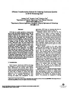
Fig. 1. Execution of a superstep by various processes. All three phases of a superstep execution are shown.

of a parallel statement, denoted by u, of a parallel algorithm. In the remainder of this paper we use the terms superstep and parallel statement interchangeably. In the study of properties of parallel algorithms, it is essenAt the beginning of the execution of a parallel statement tial to use a model M of parallel computation, which captures the main characteristics of a parallel system while abstracting (superstep), a check is conducted in order to determine which from nonessential details. In this work we have adopted a processes are enabled at the current state and which statement model of computation based on the bulk-synchronous model (which is, in fact, an update function) will be executed in each of parallel computation proposed by Valiant [ll] with some enabled process. This check can be implemented in a local or global fashion, depending on the application, and is assumed convenient extensions and restrictions. 1) An Overview of the Bulk-Synchronous Model: In the to be executed in bounded time. This check corresponds adopted model, the execution of a parallel algorithm proceeds to evaluating the guards of the update functions and may in supersteps. The processes participating in a superstep, each include a test to determine the correctness of the current one being executed on a different processor, are initially state of the computation (fault detection) in a fault-tolerant given a step of L time units to execute a specified amount implementation of an algorithm. This evaluation corresponds of processing. After each period of L time units, a global to Phase 1 of the superstep execution (Fig. 1). The system state is undefined during the execution of a check is carried out in order to determine if the superstep has been completed by all participating processes. If that is superstep. Philosophically, this is the same as viewing a the case, the computation advances to the next superstep. superstep (considering the information exchange as part of it) Otherwise, the next period of L units is allocated to the as a state transition (or as an atomic action). Therefore, the unfinished superstep. The model assumes the existence of state of the system is defined only between supersteps. We divide the supersteps of a fault-tolerant computation facilities for a barrier synchronization of processes at regular intervals of L time units, where L is the periodicityparameter. in two types: (i) normal supersteps, which correspond to the The value of L may be controlled by the program, even at execution of the original calculations of the algorithms and runtime. This mechanism captures in a simple way the idea of are composed of one step; and (ii) recovery supersteps, which global synchronization at a controllable level of coarseness execute a recovery procedure and are composed of various and it can be implemented in software or in hardware. steps. The recovery procedure embodies fault location (which A hardware realization would provide an efficient way of may have several rounds, each implemented by a step, until implementing tightly synchronized parallel algorithms without consensus is reached), when necessary, and fault recovery (which may include configuration). This classification depends overburdening the programmer. 2) Adapting the Bulk-Synchronous Model: In the context of on the result of the first phase of the superstep execution. our definition of a parallel algorithm, a superstep consists If no faults are detected in this phase, the second phase of the application of the set of update functions U to a (Phase 2 in Fig. 1) will correspond to the execution of a given state of a computation, yielding the next state of the normal computation. Otherwise, a recovery procedure will be computation. The participating processes of a superstep are executed. The final phase of a superstep execution (Phase 3 in Fig. those that are enabled in the state that precedes the execution of the superstep. A superstep is therefore formed by the 1) consists of the synchronization of processes before starting parallel synchronous execution of the update functions ui the next superstep. Information can only be exchanged among processes at the of the processes that are enabled at a given state of the computation. As the application of U to a given state 5’ end of a step. This information exchange can be accomplished corresponds to the execution of one statement in each enabled either by shared memory access or by message passing and is process, we say that a superstep corresponds to the execution assumed to be accomplished in bounded time. It is considered

B. The Parallel Model of Computation

LARANJEIRA et 01.: NESTED-PREDICATESCHEME FOR FAULT TOLERANCE

1307

The consensus-based framework for responsive (both faultto be part of a step execution. Since normal supersteps are composed of only one step, we can say that for normal super- tolerant and real-time) computer systems design was presented step executions information will only be exchanged between in [14]. supersteps. 4) The Reason for Choosing a Deterministic Model: A deterOne reason for implementing normal supersteps with only ministic model was preferred largely for the sake of simplicity one step is to guarantee that fault propagation is avoided in and potentially higher performance. A nondeterministic model cases in which processing or communication faults occurring would need to evaluate the guard of each statement of each during a superstep execution could potentially contaminate the process in order to determine which statements in each process entire computation. In such cases, fault detection is executed are enabled in a given superstep. This represents a performance at the beginning of some (or all) supersteps as part of the advantage for the deterministic model in which, once one evaluation of the guards of the update functions. If a fault is statement guard evaluates to TRUE in a process, the guard detected, the current superstep will execute a recovery function evaluation for that process is concluded. Furthermore, nondethat includes fault location (when necessary), faulty recovery, terministic models often need a mechanism to choose between and reconfiguration (when necessary). Thus, contamination two or more statements of a process that may be enabled in can be avoided and the fault tolerated. As a result of this a certain state of the computation. Both the execution of this mechanism, both communication and computation faults can mechanism and the possibility of choosing a statement to be be considered. This fault detection procedure corresponds to executed, that may lead to a less efficient solution path, can the evaluation of the predicates related to fault tolerance add a performance penalty to the execution of the algorithm. With a deterministic model, the designer can design the code defined in Section VI. Another reason to have a normal superstep implemented in such a way that in each process the statement chosen to be with only one step is to avoid an excessive performance executed next will always lead to the most efficient solution penalty due to synchronization, especially if synchronization path. This approach avoids the performance penalty inherent to known nondeterministic implementations. is realized in software. It is assumed that no faults occur during the superstep executing a recovery procedure. Therefore, fault detection is Iv. EXPRESSING PROPERTIES OF ALGORITHMS not conducted between the steps of the recovery superstep. 3) Reasons for Choosing a Synchronous Model: While an Our approach to express properties of algorithms follows asynchronous model is theoretically more appealing, a syn- the philosophy and syntax as used by Chandy and Misra in chronous model is more practical for the following reasons: Unity [ 5 ] . We study properties that are associated with the Global State Based Fault Detection and EfJiciency: In some entire algorithm, and not those that hold when control reaches cases fault detection is not possible unless the fault detection specific points of the code. However, our model of parallel procedure has access to the global state of the computation. In computation is different from the one adopted in Unity. For an asynchronous system a global state of the computation can instance, in our model, a statement is not necessarily executed only be known through a snapshot algorithm [12]. This fact indefinitely often as in Unity, and the statement guards are, causes two major problems. First, the global state provided by process-wise, mutually exclusive. As a consequence, since we the snapshot algorithm is not necessarily the one that actually used some logic relations defined in Unity, we had to adapt occurred (it is a consistent one). Therefore, fault propagation them to our model. Furthermore, we also defined some logic may be unavoidable when fault detection (and recovery) must relations that were not defined in Unity, namely the relations be executed immediately after a fault occurs (the global state degrades-to, enforces, and upgrades-to. that actually occurred is needed but it is not available). The The terminology adopted in this work denotes a parallel second problem is one of efficiency. The snapshot algorithm algorithm by A, and a parallel statement by n. G,, the guard will need to be superimposed onto the original algorithm, in of the parallel statement c7, is a conjunction of the guards of the addition to other transformations necessary for fault tolerance, process statements composing g. State predicates are denoted in order for global states to be available for fault detection by p and q. A generic system state is dentoed by S. With [8]. Since our goal is to contribute to the design of responsive respect to a computation C,So and Sk are, respectively, the systems (which combine fault tolerance and real-time con- initial state of the system, and the state of the system after the straints), the extra performance overhead that is implied by execution of the kth superstep. We denote that a predicate p this procedure may be unacceptable. holds at a state S of a computation by p 0 S. Consensus for Fault Diagnosis: The execution of fault diWe list now some logic relations that state safety properties agnosis (fault location) is clearly a consensus problem. As as well as progress properties of algorithms. Informally, a discussed by Turek and Shasha [13] the combination of safety property states that “something bad will not happen,” asynchrony and fail-stop (crash) faults makes consensus im- whereas a progress property states that “something good will possible unless interprocessor communication is ordered and a eventually happen.” Examples of safety properties could be: hardware mechanism for atomic broadcast is available. Since variable x is always nonnegative; two processes are never in fault diagnosis is absolutely essential for tolerating permanent their critical sections simultaneously. Examples of progress hardware faults (crash and noncrash), as well as certain types properties could be: variable z will become positive; process of temporary faults, we chose to have a synchronous model in p l will eventually enter its critical section. Usually a universal quantifier is used in the definition of a safety property, whereas order to have a relatively simple solution for consensus.

1308


an existential quantifier is used in the definition of a progress property (see [5]).The logic relations to state safety properties are: stable, invariant, and degrades-to. The logic relations to state progress properties are: triggers, enforces, leads-to, and upgrades-to. For a given algorithm d,the safety properties stable p , invariant p , and p degrades-to q are defined as follows: stablep E (Va : g i n A :: { G, A p } a { p } ) invariant p ( p 0 So)A (stable p ) p degrades-to q

=p 1 q z ( p + q )

V. REASONING ABOUTALGORITHM COMPOSITION

A(Va:aind:: {G,Ap}a{lpAq})

A stable predicate holds permanently, that is, is permanently equal to TRUE, once it starts holding at some point of the computation. However, it could never hold. An invariant predicate is one that is stable and holds at the initial state. Therefore, it always holds in the computation. The relation defined by p degrades-to q indicates that the execution of any statement of the algorithm causes a certain property p not to hold any more. This undermining of this property happens, however, in a controlled fashion, since a weaker predicate q , which is implied by p , continues to hold. For a given algorithm A the progress properties p triggers s , p enforces q , p leads-to q , and p upgrades-to q , are defined as follows: ptriggersa = p

.c)

g

zp

+ G,

penforcesq = p D q = ( p @ S ' )

+ ( q 0Si+1) (30 : a i n d :: ( p pleads-toq - p H q G (paS')

* ( 3 j :j 2

p upgrades-to q

p

Tq

2

y.t

:: q

a)A ( { p } a { q } ) )

0S j )

(la : 0 in d :: { p A i q } a { p } )

A (P A 7 7 )

Gu A ( 4 + P )

The expression p triggers r~ means that whenever predicate p holds, the guard G, of the parallel statement D evaluates to TRUE . Since statement guards are mutually exclusive, this implies that, whenever p holds, a is the statement that will be executed in the next superstep. The property p leads-to q conveys the notion that whenever predicate p holds, during a computation, either predicate q also holds, in which case p 3 q , or q will hold after the execution of a finite number of supersteps. If p does not imply q we can say that (341, q 2 , .

algorithm 0,which will be executed after a finite number of supersteps and which causes a stronger predicate q , such that q + p , to hold. This property expresses a diametric idea to the safety property q degrades-to p . As shown in Section VI, the newly defined logic relations degrades-to and upgrades-to serve the purpose of formalizing the notions of fault occurrence in the presence of redundancy and of fault recovery.

. . ,qm : (41 = P ) A (qm = n) A ( m 2 2)

:: 41 D q 2 D . . . D qm).

A special case of p leads-to q , when m = 2, is called p enforces q . In this case the predicate p triggers a particular statement of the algorithm which, once executed, causes predicate q to hold. It also means that if p holds in a certain state of an algorithm computation C , predicate q will hold in the next state. Finally, p upgrades-to q declares that if predicate p holds in a certain state of a computation C, there is a statement of the

The well-known concept of modularity in software engineering indicates that a large program should be composed of a number of smaller component programs called modules. Therefore, it is desirable to be able to handle one module at a time. Understanding the particular properties of the individual modules and properly defining the ways they interact greatly facilitates designing the overall program according to specifications. Our programs represent algorithms and our goal is to be able to design fault-tolerant parallel algorithms in a modular fashion. More specifically, we would like to cleanly separate functional and fault-tolerance concerns. In order to do this we address two methods of algorithm composition: superposition and concatenation. These are general methods of algorithm composition that can be used for parallel algorithm design and, more specifically, for fault-tolerant parallel algorithm design. Superposition, tailored to our model from Unity, consists of adding new variables, with the corresponding statements, to a given algorithm without modifying the assignments to the original variables. The addition of new variables may or not be accompanied by additional processes. Concatenation, which we define in this work, consists of joining two algorithms that contain assignments to the same set of variables. Given an algorithm, concatenating it with another is equivalent to adding new assignments to its variables and redesigning its guards so that all the guards of the composed algorithm are, process-wise, mutually exclusive. A. Composing Algorithms by Superposition Superposition may be used when one wants to build a composite algorithm in layers. In this case, the functions of upper layers can access the variables of lower layers, but the lower layer functions cannot access the variables of upper layers. Another use of superposition is to add functionality to an algorithm while preserving its properties. Given an algorithm, called the underlying algorithm, with its underlying variables, superposition is accomplished by inserting new variables, the superposed variables, with corresponding assignments, and modifying the underlying algorithm in such a way that the assignments to the underlying variables remain unchanged. Furthermore, the assignments of the superposed variables depend only on the values of the underlying variables. This definition ensures that superposition preserves the properties of the underlying algorithm while adding new properties to the composed algorithm through the superposed variables.

1309

LARANJEIRA et al.: NESTED-PREDICATESCHEME FOR FAULT TOLERANCE

TABLE I1 ALGORITHM SUPERPOSITION BY VARIABLE COMPOSITION Algorithm A.

I

TABLE I11 INVARIANTEMBEDDING THROUGH ALGORITHM SUPERFOSITTON BY PROCESS ADDITION

Algorithm A,

I

Procesa 1

I I

By this definition of superposition, the set of new variables and statements to be superposed on the underlying algorithm cannot exist by itself (its assignments depend only on variables of the underlying algorithm). However, for the sake of completeness of terminology, we call this set the superposed algorithm. It is also clear from the definition that the superposition operation is not symmetric. We denote by A S I A uthe composed algorithm formed by superposing algorithm A, onto algorithm A,. That is, A, is the underlying algorithm and A, is the superposed algorithm. Because in our model of computation each process updates only one variable, superposition may be performed in two ways. Process addition: For a new variable us, superposed onto the underlying algorithm, a process is added with statements assigning that variable. Variable composition: A new variable u, is superposed in two steps: a) it is joined to a variable from the underlying program vu forming a vector variable; and b) the assignments of the process of the underlying algorithm that updates u, are modified to update the new vector variable. The modified assignments should perform the desired updates to u, while not affecting the updates to 0,. Accomplishing superposition by variable composition is mathematically equivalent to realizing it by process addition. A simple example of algorithm superposition by process addition is presented in Table I. Algorithms A, and A, consist of a single process each. The composed algorithm A S I A uconsists of two processes. S denotes the system state corresponding to the underlying algorithm. In the example shown in Table I1 the same algorithm A, is superposed onto algorithm & by variable composition. Notice that the composed algorithm A S I A , has the same number of processes (one) as the underlying algorithm & but its statements are changed. The modifications inserted in the statements of the composed algorithm preserve the dynamic behavior of variables u, and u s , of the underlying and superposed algorithms, respectively, while conserving the guards’ mutual exclusion (Gl(S) and G2(S) are mutually exclusive by definition). The statements of algorithm A S I A , should be viewed as assigning one vector variable composed by variables vu and us. The composed algorithm shown in Table I1 is mathematically equivalent to the composed algorithm of Table I. Algorithm composition by superposition is a technique that extends the state of the underlying algorithm by the addition

Algorithm A, Process 2

1

[

Prom3

I

1

Algorithm A, Proc€ss 1

I

of new variables. This technique can be very useful for adding safety properties such as invariants to an algorithm. Since the assignments of superposed variables depend only on the underlying variables, one could design these assignments in such a way as to establish relations among the variables of the algorithm that will hold during the whole execution of the algorithm, provided that they hold in the initial state. This fact about algorithm superposition will be extremely useful for us when we study the design of fault-tolerant parallel algorithms in Section VII. We call the operation of adding an invariant property to an algorithm invariant embedding. In Table 111, we present an example of invariant embedding through algorithm superposition. The superposition is accomplished by process addition. The table shows the underlying algorithm A, with three variables V I , 212, and 213. The superposed algorithm A, introduces an extra variable w,, which establishes the invariant relation (w, = u1 uz 03) in the composed algorithm. The superposition is accomplished by process addition. In this case the invariant introduced is a checksum, but it could also be another type of invariant relation.

+ +

B. Composing Algorithms by Concatenation Concatenation is an algorithm composition technique that may be used to insert or enforce some desirable properties on the variables of an algorithm. Suppose we have an algorithm Ab, called the base algorithm, which is missing some desirable properties. One could concatenate it with a second algorithm At, called the tail algorithm, and form the concatenated algorithm Ab o At, which meets those properties. The tail algorithm does not have any new variables; its variable set (state) is the same as (or a subset of) the variable set of the base algorithm. When concatenating two algorithms the properties of the tail algorithm are preserved, while those of the base algorithm may be modified. This is accomplished by appending the statements of the tail algorithm to the base algorithm and redesigning the guards of the statements of the base algorithm to make all the guards of the statements of the concatenated algorithm process-wise mutually exclusive. Notice that the guards of the tail algorithm are not changed in the concatenation process, indicating that the statements of the tail algorithms will have priority over the statements of the base algorithm. That is, whenever a certain state triggers a certain statement of the tail algorithm, the same


1310

Algorithm Ab

Algorithm AI

[C,(S)l u := w(S) [Ca(S)]u := ua(S)

[C3(S)]u := U3(S)

using the definitions of stable, G i , one can safely state that

d b

and

di,ffb and ai, Gb and

+-(stable p in Ab) V (vffb: o b in d

stablep in A;

* Gb A ({Gb Ap}ffb{lp)) (P *

b

Ap

::

Therefore, we have the following. state will trigger the same statement (which belonged to the tail algorithm) during the execution of the concatenated algorithm. It is the responsibility of the designer, when redesigning the guards of the base algorithm, to make sure that the properties of the base algorithm are unchanged while the new desirable properties are added. It is also clear from our definition that the concatenation operation is not symmetric. An example of the concatenation of two algorithms is shown in Table IV. For the sake of simplicity both algorithms Ab and dt,and consequently Ab o At, have only one process. Notice that the guards of the statements of were modified in the concatenation process in such a way that a statement of Ai will only be triggered if no statement of At is. We can now study the properties of the concatenated algorithm in terms of the properties of the base and the tail algorithm. First we need to establish some terminology. We denote the guard of one statement of the base algorithm by Gb, and by G i the same guard after it is modified through the concatenation process. In the same manner, Ai is the base algorithm after the guards of its statements were modified in the concatenation process. Also, we use f f b to denote a parallel statement of algorithm Ab, and ffi to denote a parallel statement of algorithm A i . We use Gt to name the guard of a parallel statement of the tail algorithm. Let us first look at composing safety properties: Theorem 1:

0

Proof: p l q i n A b o d t =(vff:ffinAboAt::{G,Ap}o{~pAq})

*

A (P q) =(V'a:ainA;l :: {G,Ap}ff{~pAq}) A (Vo : UinAt :: {Go A p } a { - p A q } )

1) stable p in Ab o At = ((stable p in d b ) v ( V f f b : ffbinAb A p

* Gb A ({Gb Ap}ffb{lp}) (p

A (P + 4)

=(p

::

+ 1 G i ) ) ) A (stablep in At)

Proof: stablepin& o At = (Vu : a i n Ab o At :: {Go Ap}a{p}) =(Vu : a i n A i :: {G, Ap}a{p})

= ( p 1 qinAb) A ( p 1 qinAt).

0-

Now let us look at composing progress properties. Theorem 2:

1) p

6

a i n AboAt = ( ( p A~

(Va : a i n A t :: {G, A p } o { p } ) = (stablepinAz) A (stablepinAt) A

The stable property depend on the guards of the algorithm statements, as its definition states. It is easy to see that (stable p in Ab) + (stable p in A i ) . The converse, however, is not true, as shown by the following scenario. Imagine a statement 0; of di that has a guard G i that is not triggered by p . This statement does not prevent the property stable p of holding in d b o At. However, suppose it is true that the assignment corresponding to statement u t , which is the same as the assignment of statement a b of algorithm d b , does not preserve

I q i n d i ) A ( p 1 qinAt)

y+

abin Ab)

( utp ct in At)) V ( p

.c)

ot in At).

Proof: p

ut

oAt = (p

ut

c$inA;)

V (p

otinAt).

By construction of di in the concatenation process: p

y+

0

At = ( ( p -+

v (p

ffb i n d b

.c)

A l(p gtinAt).

6

fft in At)))

2 ) p D q i n d b o At =((pDqinAb) A l ( p ut ot in At)) V ( p D qin At).

0


1311

Proof: Applying a similar reasoning as done in Item 1 of Theorem 1 one can show that

communication links) for handling permanent hardware faults. Since it is well known that most of the faults that do occur in computer systems are temporary, the necessary amount of p D q i n A b o A t = (pDqind:)V(pDqinAt). spare hardware would be small, but this amount does depend on the particular system requirements and characteristics. By construction of A; in the concatenation process: In order to formally account for permanent faults we can pDqinAb o At = ((PDqinAb) A 1 ( p v+ a t i n A t ) ) extend the state of the system to reflect not only the value of V (pDqinAt) 0 the variables but also the state of the processes. The state o f a process may be up or down depending on whether the process 3 ) p H gin& p w qinAb o At is able or not to execute its update function. Formally, this can Proof: When an algorithm Ab is concatenated with an be viewed as if each process p; would have a "value" from a algorithm At, if p H q in Ab o At, nothing like p H q can domain DP equal to { up, down}. We can view the state ofthe be said about the individual algorithms Ab and At. This is variables S", composed by the state of all system variables w;, because the guards of Ab are modified in the concatenation as an element of all the set D", which is the Cartesian product process and it is possible that, even though the property does of all 0:. Similarly, the state of the processes S P , composed not hold in the individual algorithms, it holds in the composed by the state of all system processes p i , is an element of the one. However, since the guards of At have priority over the set DP, which is the Cartesian product of all 0:.The system guards of Ab in Ab o At, it is safe to state that: state S, now composed by S" and S P , is an element of the set SS, which is the Cartesian product of D" and DP. So, the p H qinAt + p ++ qinAboAt 0 state of the system reflects not only the value of the variables but also the state of the processes.

+-

0 A. Processor Faults Proof: Similar to 3. One can see from Theorem 1 that, in order to add safety properties to an algorithm Ab using concatenation, one still depends on some properties of Ab itself, which may or may not be present. Therefore, concatenation may not be a good method to insert safety properties to an algorithm. On the other hand, Theorem 2 shows that each one of the progress properties defined in Section IV, if not present in algorithm Ab, can be introduced by concatenating algorithm Ab with an appropriate algorithm At, independently of the properties of Ab. Therefore, concatenation is a good method for inserting progress properties to an algorithm. We call the operation of adding a progress property to an algorithm progress securing. As will be shown in Section VII, progress securing by algorithm concatenation can facilitate the design of fault-tolerant parallel algorithms. VI. A GENERALMODELFOR FAULTTOLERANCE When studying fault tolerance we are faced with myriad existing techniques that aim to solve the same problem by different means. Among these we could mention: replication and voting [15], checkpointing and rollback [16], algorithminherent fault based fault tolerance [ 171, self stabilization [MI, tolerance [19], and natural redundancy [3] (see Section VI11 for discussion). In Nest we intend to uncover the underlying commonality among these diverse methods in order to propose a general model for fault tolerance, as well as a methodology for designing fault-tolerant parallel algorithms. In this research, we assume that each process is executed on a different processor. The algorithm is fault-free. There are no software design faults. We attempt to model the tolerance of hardware faults, single or multiple, permanent or temporary, that affect processors or communication links. We consider the availability of some spare hardware resources (processors or

During the computation of an algorithm the occurrence of a fault is a probabilistic event. We model the occurrence of a processor fault fi from a set of faults f , by the execution of a parallel statement vf of the algorithm. The guard Gf of such a statement is conditioned by a probabilistic predicate 3i.The probabilistic predicate 3 is a conjunction of all probabilistic predicates 3i,each one corresponding to a fault in a different where m is the processor. That is, 3 = 3 1 V 3 2 V . . . V 3m, number of faults that can occur. A fault-free computation is one during which 13always holds.

B. Communication Faults A communication fault is also modeled by the execution of a statement of the algorithm. When a communication fault does occur, the processor receiving the faulty message or faulty shared memory access will not a see correct state of the computation. Existing fault-detection techniques check correctness using intermediate computed values communicated from one processor to another. Regardless of how a computed value was corrupted the fault will be detected. The model need not distinguish between processor and communication faults because the result seen by the receiving processor is the same. If the fault is permanent one can use existing fault-location algorithms that can distinguish processor and communication faults (see [20] and [21]) in order to know which hardware resources must be replaced before recovery is executed. C. Timing, Omission, Crash, and Synchronization Faults Timing, omission, and crash faults can be either processor or communication faults. The standard procedure for detecting these kinds of faults, which we also adopt, is the use of watchdog timers. A timer is set to go off after the amount of time in which a certain calculation is supposed to be accomplished. When the calculation is completed the timer

1312

is switched Off. If the timer goes off (obviously before the calculation is accomplished), a timing, omission, or crash fault has occurred. Recovery then follows. Although timing, omission, and crash faults can cause synchronization problems, we would like to call synchronization faults those faults that involve the synchronization mechanisms. In the case of a bus-based shared-memory multiprocessor system, an incorrect update of a synchronization variable could cause this type of fault. A synchronization fault will deadlock the processes involved in the computation. This fault can also be detected with watchdog timers. In certain cases, the best recovery method may be simply to execute a retry in the superstep in which the fault occurred after the previously correct state is restored.

D. Faults in the Evaluation of the Guards of Process Statements A fault in the evaluation of the guards of the process statements is basically a processor fault that will cause either the wrong statement of a process or no statement at all to be executed (when one should be executed). If the wrong statement is executed, the system will interpret it either as a simple processor fault or as a synchronization fault (in case a recovery statement is incorrectly executed). If no statement is executed in the process when one should be, this will be interpreted by the system as an omission fault (if a message is not sent, for instance) or as an incorrect computation fault (if, for example, the value of a variable in shared memory is not updated).

E. Reasonable Computations Another assumption of the Nest model is that we will always have a reasonable computation. A reasonable computation CR is one during which, if faults occur, the fault frequency is such that the computation will succeed in reaching a fixed point. The reason for this assumption is that, in the worst case, the fault frequency could be high enough (and uniformly so) that all the computation time of the machine would have to be allocated to the execution of recovery procedures. This would prevent the computation of the algorithm itself from making progress toward a fixed point if the recovery scheme is not forward recovery. The assumption of a reasonable computation allows the fault frequency to be high for some time, but not continuously high. That means that the fault frequency will eventually decrease, allowing the computation to make progress toward reaching the fixed point. If the fault frequency becomes high again, it will decrease again later. This way, our assumption is that, even in the worst case, the computation will still reach convergence. We would like to formalize the notion of a reasonable computation. Since we deal in this work only with convergent computations, a computation is always considered to have a nonempty set of fixed points FP that will be reached in fault-free situations. An interval [sa,&,] of a computation, with b > a, is a subsequence of states of the original computation having Sa


as its initial state and sb as its final state. We define the distance between two states sa and sb of a computation dist ( S a ,S b ) , with b > a , as the number of SUperstep executions that separate s, and S b in the computation (whether it is affected by faults or not). The fault-free termination distance of a state Sa of a computation ff-dist ( S a )is the distance from Sa to a fixed point in FP, considering that no faults occur during the computation of the interval [ S a F , P]. An interval sb]of a computation is said to be profitable if the relation ff-dist < ff-dist ( S a )holds. Any interval of a convergent computation in which no faults occur is profitable, assuming that the execution of each superstep causes the computation to make progress toward a fixed point. An interval [sa, sa]is nonprofitable if faults occurring during its execution cause ff-dist (56)> ff-dist ( S a )to hold. Finally, a reasonable computation C n is one during which the fault frequency is such that for each and every state Sa in C n , Sa not in FP, there exists a state S b in CR-b > a such Sb]is profitable. that the interval [S,,

[sa,

(sa)

F. Nest Fault-Tolerance-RelatedState Predicates Intuitively, two features must be present in an algorithm for it to be fault tolerant. First, it must possess some form of redundancy. This implies that the results of the algorithm should be achievable in diverse but equivalent ways. Second, the algorithm must be able to use this redundancy, in the event of a fault, to ensure that the expected results of its execution will still be delivered. We would like to have a formal way of expressing these intuitive attributes of a faulttolerant algorithm. A first step is to notice that these attributes can be expressed in terms of safety and progress properties of the algorithm. The characteristic of being redundant can be expressed as a safety property. On the other hand, the ability of using redundancy in order to ensure the correctness of the final result in the presence of faults can be expressed as a progress property of the algorithm. We now define the three predicates, which constitute the heart of the Nest model, that will allow us to express formally the algorithmic properties related to fault tolerance. These predicates are: correct, safe, and recoverable. Fig. 2 shows a diagram representing the set S S of all possible system states and the states at which these predicates hold. From this diagram we can see that correct 3 safe, safe + recoverable, and, applying transitivity, correct + recoverable. We define a correct predicate as one that is given by the specifications of the application and characterizes the correctness of the states of a computation. Correct is stable in the absence of faults. A safe predicate is one that holds in a state that, as the computation proceeds from that state, and supposing no more faults occur, it will reach a correct state in a finite number of supersteps without executing a recovery procedure. A correct state is also safe, but a safe state is not necessarily correct. So, safe is also stable in the absence of faults. A fault may cause a computation to go from a correct state to a state that is safe, but not correct [see Fig. 3(b)]. A computation passing

LARANJEIRA et aL: NESTED-PREDICATE SCHEME FOR FAULT TOLERANCE

ss

1313

be executed in the next superstep. In practice this assumption corresponds to the use of existing fault-detection algorithms that are available in the literature. Fault detection can be done with hardware aid (component replication with a hardware comparator, self-checking logic, watchdog timers, error detection codes, and so on), by using replication and comparison of computations (with or without hardware replication), or exploiting properties (invariants) of the application.

G. A Definition of a Fault-Tolerant Algorithm

Fig. 2. Nested system-state predicates for modeling fault tolerance. SS is the set of all possible system states. The region in black corresponds to nonrecoverable states.

through safe but not correct states will converge either to the same fixed point that would be reached in case of no faults, or to a different one that also meets the system specifications [see Figs. 3(b) and 3(c)]. A safe state could be used as a valid initial state of the computation. The recoverabze predicate expresses the profitable utilization of redundancy. A recoverable state is one that, even when it is partially contaminated by faults, it is still healthy enough (due to redundancy) to be restored to a safe or correct state through a recovery procedure [see Figs. 3(c) and 3(d)]. Notice that a safe state is also recoverable, as is a correct state. A correct or safe state can be viewed as a recoverable state for which the recovery procedure is an empty statement. However, there may be cases when it might be interesting to use a recovery procedure to upgrade a safe state to a correct one or to another safe state which is “closer” to the fixed point. This is purely a performance issue and not one of correctness. A “closer” state will simply converge faster. A nonrecoverable state is one that is so contaminated that it cannot be restored. A computation that reaches a nonrecoverable state because of faults will not converge [see Fig. 3(e)]. This is because there is insufficient redundancy. In Fig. 2 the dark area represents the nonrecoverable states. The properties degrades-to and upgrades-to, defined in Section IV, formally capture the dynamic behavior of an algorithm execution with respect to the predicates we just defined. A transition from recoverable to safe, or from recoverable to correct, is expressed by upgrades-to. A transition from correct to safe, from correct to recoverable, or from safe to recoverable, is expressed by degrades-to. In the context of this work, we only consider valid initial states, that is, those states that satisfy the application specifications and for which the algorithm converges. Both the predicates correct and safe (and consequently recoverable) hold for any valid initial state. Therefore, correct and safe are invariant in the absence of faults. It is also an assumption of the Nest model that the predicates just defined can be checked as to whether or not they hold, in order for the system to decide which parallel statement will

We now present a definition of a fault-tolerant algorithm: Definition 1: Given the predicates correct, safe, and recoverable as defined previously, we say that an algorithm .Aft is fault-tolerant with respect to a given set of faults f , if and only if, during an execution of this algorithm in which all faults occurring are from the set f , the following properties hold: e invariant recoverable e recoverable upgrades-to safe. The model and stated definition are general since no limitations are placed on the set of faults f that a fault-tolerant algorithm can tolerate. Existing techniques for fault tolerance, however, are quite different in their scope and applicability. For instance, an algorithm designed with triplication and voting (triple modular redundancy) will be able to tolerate single or multiple faults, permanent or temporary, provided that no two faults occur in a pair of processors (and communication hardware) simultaneously. An algorithm designed with checkpointing and rollback recovery will be able to tolerate single or multiple faults, but only those that are temporary. Finally, an algorithm designed with the algorithmbased fault-tolerance technique will be only able to tolerate single temporary faults. When applying a particular technique one must be aware of its limitations. The first property (invariant recoverable) says that the predicate recoverable always holds during the computation (we have assumed it holds in the initial state). If a fault occurs while the computation is in a correct or safe state, the resulting state will be recoverable. Furthermore, if a fault has occurred that caused the system to be in a state where the predicate (recoverable A 1 safe) holds, either no additional faults occur until a recovery procedure causes the computation to reach a state where safe or correct holds, or, if statements of the original algorithm are executed and/or subsequent faults occur before recovery is accomplished, recoverable still holds in the resulting states. The second property (recoverable upgrades-to safe) says that during the course of a computation safe eventually holds after a fault forces the system into a state where (recoverable A T safe) holds. This property ensures that some recovery procedure is executed to upgrade a recoverable state to a safe (or correct) one. We say that a recovery procedure will eventually be executed in order to be able to model faulttolerant systems that, after a fault occurs, continue executing for some time until the fault is detected and the recovery procedure executed (e.g., systems using the checkpointing and rollback technique). There are other cases, however, where the recovery procedure must be executed in the superstep immediately after the fault occurrence. This is necessary in

1314


I

Fig. 3. (a) A computation with no faults. All states are correct. @) A computation in which a fault causes a safe state to be reached. (c) A computation in which a fault causes a recoverable, but not safe, state to be reached. An explicit recovery action brings the system back to a safe state. (d) A computation in which a fault causes a recoverable, but not safe, state to be reached. An explicit recovery action brings the system back to a correct state. (e) A computation in which a fault causes a nonrecoverable state to be reached. The computation does not converge even if a recovery action is attempted.

TABLE V PROPERTIES OF ALGORITHMS A i t AND F I'ropertia of A;,

1

Properties of F

I cornct ncouemble upgrades-lo sale invariant

I

cortact degrades-lo ncoveroble saJe degrndes-lo n c o n c r o b l e invanant ncoveroble

I

order to prevent fault propagation and, consequently, to avoid reaching a system state that is so damaged that it cannot be restored. An example of this is a system made fault tolerant with a technique that can only tolerate single faults. In such a system, immediate fault detection is a must in order to avoid, for example, the contamination of the data space of several processors when one processor is faulty and its partial results are communicated to the others. After the fault is detected, fault location must be executed for the system to know which portion of the system state must be restored. Fault location is also a must, in order to locate the faulty processor for the sake of executing reconfiguration, when crash or permanent faults happen. Therefore, we argue that our defined recovery procedure embodies fault location (when necessary), fault recovery, and reconfiguration (when necessary). As stated earlier, we view a fault-tolerant algorithm Aft as a combination of a set of statements modeling faults, called F, and a set of statements corresponding to the real computation, called Table V shows the properties of A;t and F that are related to fault tolerance. The faults modeled by F are those that dftcan tolerate.

VII. A GENERALMETHODOLOGY FOR THE DESIGN OF FAULT-TOLERANTPARALLEL ALGORITHMS In view of the theoretical foundation for fault tolerance laid

in the previous sections we are now prepared to propose systematic principles that constitute the Nest design methodology for reliable applications running o n multiprocessor machines. The principles proposed in this section are only applicable to the fault-tolerant aspects of a design. We assume that functional aspects are handled by appropriate methods. We can list three major tasks in the design of a fault-tolerant parallel algorithm for a given application: Clearly state fault-tolerance-related system requirements and limitations, and assess system characteristics. Investigate whether the application (or an existing version of the algorithm) has inherent characteristics that cause some (or all) of the fault-tolerance properties related in Definition 1to be met. If such properties exist, check whether the fault tolerance thus provided meets the requirements of the previous step. If properties exist that meet all requirements, stop; otherwise, execute the next procedure. Apply general techniques through which the existing version of the algorithm may be transformed in order to meet the missing properties and desired fault-tolerancerelated requirements. the first task, the designer should prepare complete specifications for fault tolerance and verify requirements such as: a) what classes of faults must be tolerated by the system; b) what the acceptable cost levels are in terms of space and time overhead, that the system can bear in order to achieve fault tolerance; c) what the threshold values are for quantifiable dependability criteria. In the second task, the designer will check if the application (or an already existing version of the algorithm) is inherently fault tolerant, self stabilizing, has some natural redundancy,


or has any other characteristic that could facilitate the incorporation of fault tolerance. If this is the case it is still necessary to ensure that the fault tolerance resulting from these properties meets all systems requirements. For instance: a) If the intrinsic characteristics of the algorithm enable it to tolerate fail-stop faults, but multiple temporary faults are expected to affect the system, still another technique for fault tolerance that can handle temporary faults must be used; b) If the intrinsic characteristics of the algorithm enable it to tolerate the classes of faults stated in the requirements but with higher time overhead than the system can bear, a still more time-efficient technique for fault tolerance should be used; c) If the algorithm has natural redundancy, that redundancy still needs to be exploited for fault tolerance by the implementation of a recovery procedure. In summary, if some or all of the desired properties are missing or existing properties do not meet system requirements, the designer should execute Task 3. In the third task, the designer should apply systematic transformation methods to an algorithm in order to add the missing fault-tolerance properties that cause the desired techniques to be met. These systematic transformations can be accomplished by the algorithm composition techniques studied in Section V. In order to insert redundancy one would utilize the invariant embedding technique, which can be implemented by algorithm superposition. The practical issue here is to provide an invariant embedding that is both feasible and efficient to compute. Here again the specific characteristics of the application may facilitate one approach over several others. In order to add recovery procedures one would utilize the technique we called progress securing, which can be implemented by algorithm concatenation. Note that the type of redundancy (inherent or inserted into an algorithm) will largely determine the recovery procedures that may possibly be implemented. In the next section it is shown that the proposed design principles are at the heart of existing techniques for fault tolerance. Two practical examples of the application of this methodology are also presented.

1315

fault location (when necessary), recovery, and reconfiguration (when necessary). Nevertheless, for the sake of simplicity, only recovery statements are shown in the examples. We also assume that faults do not occur during the execution of the recovery procedure. With this assumption, the restriction that information exchange can happen only at the end of a superstep can be relaxed for the superstep corresponding to the execution of the recovery procedure. Although we do not focus on specific fault-detection and fault-location (diagnosis) algorithms, efficient solutions for these problems can be found in [20]-[27]. A. Theoretical Examples

In this section, we are only interested in the fault-tolerant aspects of algorithms that are designed with a set of different techniques for fault tolerance. Functional aspects are not considered. The techniques we cover are those listed in Section VI: replication and voting [ 151, checkpointing and rollback [ 161, algorithm-based fault tolerance [ 171, self stabilization [18], inherent fault tolerance [19], and the approach based on natural redundancy [3]. We provide a brief description of each technique. We encourage the interested reader to refer to the references for more details. In each example, we present a table showing: 1) the basic or normal algorithm; 2) a step-by-step description of the transformations undergone by the algorithm in order to model faults and to add redundancy (invariant embedding) and/or a recovery procedure, when applicable; and 3) the fault tolerance properties met by the resulting algorithm. System requirements are not considered in the theoretical discussion of this section since we are focusing on the properties introduced by the techniques for fault tolerance and not in the specific algorithms or computational environments. Replication with Voting: In this technique, processors and communication hardware are replicated. After each superstep the results computed by the processors in each set of sibling processors are compared and a majority vote is taken to choose the correct result. The voting procedure takes care of both fault detection and recovery. The technique works as long as a majority of processors (or communication hardware) in each VIII. APPLYING THE MODELAND DESIGNMETHODOLOGY replicated set is not simultaneously faulty. Both temporary and We can now show the applicability of the Nest model and permanent faults can be tolerated by using replication with design methodology for fault tolerance. We do so by focusing voting. Table VI presents a customization of our model and deon theoretical and practical examples. At first we examine a set of existing techniques for fault tolerance. We demonstrate sign methodology for a fault-tolerant algorithm utilizing the that the proposed model provides a common ground for all of replication with voting technique. The normal algorithm in them and that they are instances of utilization of the design the example has only one process and one variable, but procedures outlined in the previous section. Then we give two it could have several. Invariant embedding is executed by practical examples of how the presented model and design triplicating the processes (and the corresponding hardware). methodology are used to insert fault tolerance into two specific Progress securing (recovery) is added by the voting procedure. If no fault occurs in a superstep, all can be viewed as if each algorithms. It is worth noticing that in all of the examples that follow, variable in a triplet retains its value (since they are all equal). algorithm statements modeling faults are inserted through The fault tolerance properties of the algorithm show that the algorithm concatenation. The predicate F P indicates that the occurrence of a fault causes the predicate (recoverable A i computation has reached a fixed point or has converged. Fault safe) to hold. As a result, the recovery procedure is executed detection is modeled by the evaluation of predicates cor- in the next superstep and it restores the faulty state to a state rect, safe, and recoverable. The recovery procedure embodies where the predicate correct holds.

1316


TABLE VI ALGORITHM WITH TRIPLICATION AND VOTING AND ITS FAULT-TOLERANCE PROPERTIES EXAMPLE w

m TRIPLICATION AND VOTINQ Normal Algorillm Process 1

[-FP]

vi

:= ui(S)

[TFP] vi := ul(S)

[-FP]

y

:= w(S)

I

Adding Fault Modcling by Algorithm Concatenation Process 1 ProceM 2

Adding Fault Modeling by Algorithm Concatenation ProceM 1

I

I

Adding Redundancy (Checkpoinling) by Algorithm Superparition Process 1 I Pr0ce.s 2

1

I

I

Adding Recovery (Voting) by Algorithm Concatenation I PrOCeM 2 I Pmceu 3 PTOCeM 1 [-FPh-F1;h cortecf]

[FjAcorrcctj [-correct]

VI

I

Adding Recovery by Algorilhm Concatenation Procea. 2 I

Process 1

I

I

v1

v1

:=

1

correct P ProDerties 01A I . invariant recoverable recwerable b correct

I

(VI

= tq A y = ua

inunrinnt correct recoverable b correct

~

I1

I

A v1

ProDcrtiesolA:.

~

= v3) I

Pr o o a t i n o f F

I

correct d e # n d a r - t o recoverable (recoverable A -correct) +. disabled ~~

I

~

Checkpointing and Rollback: In this technique a checkpoint of a correct state is periodically stored in stable storage. Upon the detection of a fault the last state stored as a checkpoint is restored and the execution of the application restarts from that state. This technique is normally used to tolerate temporary faults. Table VI1 presents a customization of our model and design methodology for a fault-tolerant algorithm utilizing the checkpointing and rollback technique. The normal algorithm has two processes. Invariant embedding is done using superposition by variable composition. The disk storage that contains the latest checkpoint is modeled by two new variables 'u1 and w2. The predicate C P is used to signal the supersteps in which checkpoints are taken or recovery is accomplished. S+ stands for the system state, including the new variables added to store the checkpoints. A state contaminated by a fault will be restored during the execution of the next superstep, after the fault occurrence, in which C P holds. Depending on the frequency with which checkpoints are taken (dictated by C P ) the time overhead necessary to recover from a fault could be considerable because of recomputation (rollback). The recovery procedure restores the computation to a state in which the predicate correct holds. Algorithm-Based Fuult Tolerance: In this technique, mainly used with problems involving matrix operations, checksums of the application variables are added to the problem in order to allow fault detection, location, and recovery to be achieved. Algorithm-based fault tolerance has been proposed to tolerate temporary single faults. This technique could be extended to tolerate permanent single faults at the expense of additional space and time overhead. Table VI11 presents a customization of our model and

design methodology for a fault-tolerant algorithm utilizing the algorithm-based fault-tolerance technique. The normal algorithm has two processes. Invariant embedding is accomplished by introducing a checksum variable. Fault location requires a second extra variable corresponding to a weighted checksum [17]. For the sake of simplicity, we did not include the second extra variable in Table VIII, as we have assumed that fault location is accomplished during the execution of the recovery procedure. Recovery can be viewed as a function of S+, which is the extended system state. The occurrence of a fault causes the predicate (recoverable A 1 correct) to hold. The recovery procedure, executed in the superstep following the fault occurrence, results in a state where the predicate correct holds. Self Stubilizution: Self-stabilizing algorithms were first noticed by Dijkstra [18] as algorithms that can tolerate temporary faults without the addition of explicit procedures to achieve fault tolerance. In the execution of these algorithms a state affected by a temporary fault will still lead to a legal state. It is assumed that as a computation continues from a faulty state a fault-free state will eventually be reached. Table IX presents a customization of our model for a selfstabilizing algorithm. The algorithm has three processes. It is worth noticing that no invariant embedding is necessary. The required redundancy is already a characteristic of the algorithm. The algorithm is redundant with respect to the initial state; that is, any state is a valid initial state. Since any state is a valid initial state, after a fault occurs the algorithm automatically restarts its execution with the state resulting from the fault as the initial state. There is also no need for an explicit recovery procedure. Recovery is simply accomplished by continuing the computation. We understand

LARANJEIRA et aL: NESTED-PREDICATE SCHEME FOR FAULT TOLERANCE

1317

EXAMPLE WLTli A L G O l i l ~ I l M - B A S E UFAULT TOLERANCE ' N o m d Algorithm

Proceu 2

Process 1

[-FP]V I := q ( S )

I-FP] y

:= uz(S)

Adding Fault Modeling by Algorithm Concatenation Proccsa 2 Process 1

I

u3

s :=

u1

s

1

+ u2 PrOCeM 2

Pmceu 3

[-FPA - 7 3 A

[-FPh-F1h

[-FP

correct] VI := w(S) [FIA correct] VI := h(S) [-correct] VI := rcct(S+)

[FzA correct] y := h ( S )

A -3zA

correct] y := 4 . 9 ) [-correct] y

:= recz(S+)

correct] v3 := u3(S) correct] VJ := f3(S) [-correct] u3 := rec3(S+) [73 A

[-FPh correct] "4

I

I

-correct)

[-FP]V I := ui(S)

I-FP]

V?

[-FP]V J := u,(S)

:= uz(S)

I

I

Adding Fault Modeling by Algorillmi Concatenation I Proceas 2 I Process 3 Procesa 1

I 1

I

Propertiead Art invariant snje

I I

I

:= u,(S)

Prooerties of A?. invorinnt correct

I I

Prooertics of F correct degradc,-to a a j c rlablr r n j c

I I

I

that the self-stabilizing property is an implicit characteristic of the algorithm. Therefore it cannot be added through algorithm composition, because the composed algorithm will be a different algorithm. In our view, an algorithm that results from an algorithm composition process and is able to tolerate faults is fault-tolerant and not self stabilizing. Notice that the predicate safe always holds during the execution of a self-stabilizing algorithm as long as only temporary faults, after which the algorithm can still stabilize, happen. One experiment described in [28], involves a situation in which a temporary fault caused a floating point exception. The running self-stabilizing algorithm could not tolerate such a fault. Inherent Fault Tolerance: Inherently fault-tolerant algorithms, noticed by Bastani et al. [19], are algorithms that have redundancy in the execution process. The processes of the algorithm independently cooperate in achieving a common goal. Therefore, if a fault occurs, causing a process to halt, the algorithm continues execution normally. The final result

a diaabled

will be reached with some performance degradation, since one less process will be cooperating to achieve the common goal. Inherently fault-tolerant algorithms have properties similar to self-stabilizing algorithms. The difference is that inherently fault-tolerant algorithms tolerate fail-stop faults instead of temporary faults. Since a fault halts a processor (and the corresponding process), we consider that an inherently faulttolerant algorithm can only tolerate faults that leave a number of processes operational, which is sufficient for the completion of the algorithm. Table X presents a customization of our model and design methodology for an inherently fault-tolerant algorithm. The algorithm has three processes. Notice that no algorithm composition is necessary to insert redundancy or a recovery procedure. The predicate safe always holds during the execution of an inherently fault-tolerant algorithm as long as the only faults to occur are fail-stop (crash) faults that can be tolerated by the algorithm. Obviously, if all processors fail by stopping, the computation cannot be satisfactorily completed. Natural Redundancy: Naturally redundant algorithms, proposed in [3], are algorithms that possess implicit redundancy in the problem variables. Even with redundancy, the algorithm is not able to automatically recover from faults. In order to restore a faulty state, an explicit recovery procedure must still be added to the algorithm. Naturally redundant algorithms are in an intermediary position between algorithms that need neither redundancy nor recovery to be added and algorithms that, in order to be made fault tolerant, need both redundancy and recovery to be inserted in their executions. This technique for fault tolerance allows algorithms to tolerate temporary and single faults. It can also be extended, by the addition of a reconfiguration procedure and the availability of spare processors, to tolerate permanent single faults.

1318


[

:::5

?

0.28

Normal Algorithm Procau 1 [-FP] v i

Process 2

:= ui(S)

[+PI

y

[-FP]

UJ

:= u ~ ( S )

I

I

Propertiesof d;,

I

I

I

Propertiesof F

I

I

invariant raje

Fig. 4. (a) Three-state Markov model; (b) corresponding transition ptobability matrix P.

I

I

Propertiea of AIl

invariant corncl

I

eorrecl degrader-lo safe atable rajc

I

TABLE XI FAULT-TOLERANT ALGORITHM EXPLOITING NATURAL AND ITS FAULT-TOLERANCE PROPERTIES REDUNDANCY REDUNDANCY Normal Algorithm I Process 2

Process 1

t

Adding Fault Modeling by Algorithm Concatenation Process 1 I Proctor 2 I

1

I

Adding Recovery by Algorithm Concatenation Process 2 Procca. 1

I

[-+PA

-FI A correct] (9-1 A

VI

correct] UI

[-correct]

VI

:= ul(S) := f1 (S)

:= i e q (S)

[-+PA

(b)

(a)

I

Adding Fault Modeling by Algorithm Concatenation I Process 2 I Proccu 3 Procau 1

1

0.72

Proem 3

:= UZ(S)

#

:::

-hA correct] y := u,(s) [FzA correct] vz := jz(S) [-correct]

tq

:= r e q ( S )

transition. As time progresses, a system goes from state to state under the basic assumption that the probability of a given state transition depends only on the current state. We are particularly interested here in the discrete-time, time-invariant Markov model, which requires all state transitions to occur at fixed time intervals and transition probabilities not to change over time. Figure 4(a) shows a graph representation of a three-state Markov model. The nodes represent the states of the modeled system; the directed arcs represent the possible state transitions; and the arc weights represent the transition probabilities. The information conveyed in the graph model can be summarized in a square matrix P (Fig. 4(b)), in which each element p,, is the probability of a transition from a state i to a state j in a given time step. Such an N x N square matrix P is called the transition probability matrix of an N-state Markov model. P is a stochastic matrix, since it meets the following properties: p,, 2 0 for 1 5 i,j 5 N , and C ~ z l p 2 = , 1 for

l < i < N . A discrete-time, finite-state Markov chain is a sequence

-correct)

$

disabled

{ X k l k = 0,1,2,. ' .} of random variables that take values in a finite set (state space) {1,2,. . . , N } such that Pr ( X k + l = j ( X k = i) = q X 3 , k >_ 0, where Pr means probability. A Markov chain chould be interpreted as the sequence of states of a system modeled by a Markov model with the probabilities qTJgiven by the entries p,, of the transition probability matrix

Table XI presents a customization of our model and design methodology for a fault-tolerant algorithm exploiting natural redundancy. The normal algorithm has two processes. Notice that invariant embedding is not necessary since the algorithm already has natural redundancy in the problem variables, which can be used for fault detection and fault tolerance. The introduction of a recovery procedure is, however, necessary. During the execution of a fault-tolerant algorithm exploiting natural redundancy, the occurrence of a fault may cause a predicate recoverable AT safe to hold. The recovery procedure, executed in the next superstep, results in a state where the predicate safe (or correct) holds.

P.

Let nobe an N-dimensional nonnegative row vector whose entries sum to 1. Such a vector defines a probability distribution for the initial state X o by means of the formula Pr ( X o = i) = T : , where each n:, 1 5 i 5 N, is an element of no. Given an initial probability distribution no, the probability distribution nk,corresponding to the kth state X k , would be given by (l), where Pk means P to the kth power.

Equivalently,

B. Practical Examples The two examples, we will describe, are the computation of the invariant distribution of Markov chains and the solution of systems of linear equations. The Computation of the Invariant Distribution of Markov Chains: The Markov process model is a powerful tool for analyzing complex probabilistic systems such as those used in queueing theory, computer systems reliability, and availability modeling. The main concepts of this model are state and state

k+l

k

One often desires to compute the steady-state (invariant) probability distribution IIss for a Markov chain. The vector IIss is a nonnegative row vector whose components sum to 1, and has the property IIss = IIss P. One way of calculating nSsis to use an iterative procedure, such as the one shown in (2), until convergence is reached. For

1319

W J E I R A et 01.: NESTED-PREDICATE SCHEME FOR FAULT TOLERANCE

a system with N states we could have N processes, each one calculating one component T ; of IT, 1 5 i 5 N . A convergence - T"-') < E } , for some criteria would be {Vi, 1 5 i 5 N I ( T ~ given E . Utilizing the proposed model the algorithm could be expressed for each process as:

And considering fault modeling:

The resulting algorithm is fault-tolerant and requires no space overhead in fault-free situations or in situations involving temporary faults. One extra superstep (time overhead), corresponding to the recovery procedure, is necessary to achieve fault recovery. The fault-tolerance properties met by the resulting algorithm as shown in Table XI are invariant recoverable and recoverable enforces safe. The Solution of Systems of Linear Equations: Systems of linear equations often appear in scientific and engineering problems. Usually, we have N unknown variables and N equations in a system represented as a matrix equation such as

N

A*X=B

(3)

j=1 / k \

Let us suppose that the probability of multiple faults occurring in the environment where this algorithm will run is very low. Therefore the algorithm must tolerate only single faults. Let us consider also that the cost of hardware replication for this system is very high, so one would want to achieve fault tolerance with minimum space overhead. Observation of the algorithm shows that it is a naturally redundant a1 orithm as defined in [ 3 ] .An invariant is already r$ n2 = 1. Therefore we do not need to insert present, redundancy, but we do need to insert a recovery procedure. This is accomplished by algorithm concatenation, resulting in N

[ ~ F AP-3% A correct]rf+l :=

C(r:* p j z ) 3=1

[F% A correct]rf+l := f i

(n* i N

[Tcorrectlrf := 1-

/

E

.rt 3=1,..#aI * recovery procedure

* /.

Fault detection is embedded in the evaluation of the predicate correct. The recovery procedure is also simplified in the above description of the algorithm. In fact, we assume that fault location, in addition to fault recovery, is embedded in the recovery procedure. In order to tolerate permanent hardware faults, spare processors must be considered, and a reconfiguration procedure must also be incorporated in the recovery procedure. When such a fault occurs, the recovery procedure locates it, activates a spare processor, creates the corresponding process, and then restores (recovers) the state of the computation. We omit details regarding fault detection and location here, but specific solutions for the Markov algorithms can be found in [ 3 ] . In particular, the fault location scheme exploited in that work uses the shifted recomputation of a superstep. This approach allows fault location to be achieved without the addition of an extra variable just for fault-location purposes, as is done in the algorithm-based fault-tolerance technique.

all a21 a31

a12

a13

" '

alN

a22

a23

...

a2N

a32

a33

' "

a3N

aN1

aN2

aN3

"'

aNN

*

bl

x1 x2 53

b2

=

XN

b3

. (4)

bN

Matrices D and E of (5) are obtained from matrices A and B of ( 3 ) and (4) in the following way: a) d;; = 0 , l 5 i 5 N ; b) dij = aij/a;i,i # j , 1 5 i , j 5 N ; c) e; = bi/aii, 1 5 i 5 N. This solution could be implemented with N processes, each one calculating one component x; of X , l 5 i 5 N . A convergence criteria would be {Vi, 1 5 i 5 NI(xf - xb-l) 5 E } , for some given E . Utilizing our proposed model, the algorithm could be expressed for each process as: [ ~ F P ] x f +:= l 1/a2,*

[ (-

N

(az3* xf)) 3 =1J

+bj] .

# Z

And considering fault modeling:

[F2]Xt+l

:= f,(X".

Let us suppose that the probability of occurrence of permanent faults in the system on which this algorithm will be executed is very low. Observation of the algorithm shows that it is self stabilizing. Since any initial state is a valid initial state, a state following the occurrence of a temporary fault (be it single or multiple) is also a valid initial state and the computation can simply continue from there. In this case, the algorithm meets the property invariant safe, as shown in Table IX, and its inherent characteristics satisfy the system requirements related to fault tolerance.

1320


However, if the system needs to meet real-time constraints, self stabilization might not be a viable fault-tolerant solution. A fault could cause a computation to reach a state that is much farther from the final expected result, in terms of the number of supersteps (iterations), than the original state. In order to have fault tolerance with low time overhead, triplication with voting could be used. Algorithm superposition could be used to add redundancy. For each component of the output vector we would have three proceses modeled as

*

*

[([(-

N

j=l,j#i (aij

N

(Uij

*%;I)

+bj]

*%;I)

+bj]

j=l,j#i

:=l/azi*

:=

7

A

~

l/Uii*

[(-

N

(uij*z;1)

+bj]

j=l,j#i

The invariant resulting from these operations is that in fault-free situations we must always have, after each superstep (iteration), xf = 2: = -Ic xi. As shown in Table VI, the resulting algorithm has two fault-tolerance properties: invariant recoverable and recoverable enforces correct. No extra supersteps are required in fault-free situations and only one extra superstep is necessary for recovery (the voting procedure is executed in an extra superstep when the replicated computation results do not match). Space redundancy (extra variables, processes, processors, and communication hardware) is, however, very high (200%). If the cost of extra hardware is prohibitive one must look for a way of inserting redundancy that can be computed with less space overhead. An alternative solution would be to add to the algorithm one extra variable, Z N + ~(and the corresponding extra process), which after each superstep (iteration) is equal to the sum of all the others. Thus, using superposition the algorithm would be modeled as

in which each predicate 3; depends only on the variables xi, 1 5 i 5 N ; each predicate 7i d e p e g s only on the variables Z;, 1 5 i 5 N ; and each predicate Ti depends only on the variables Zi, 1 5 i 5 N . For 1 5 i 5 N , predicate Fi and predicate 7 iof the replicated processes correspond to predicate 3i of an original process. Recovery could be added by algorithm concatenation resulting in the majority voting procedure:

[,FP A

[(-

*

[(-

N

(aij*x;)) +bj]

j=l,j#i

correct]xf+' ; N

i.lj*.:i)

+bj]

j=l,j#i

where

[,FP A

Gi A correct]$+'

:=l/ai;*

[(-

N

N

N

j=l,j#i( u i j * T ; ) )

Adding recovery through algorithm concatenation we would obtain

1321

LARANJEIRA et al.: NESTED-PREDICATESCHEME FOR FAULT TOLERANCE

*

[ (-

TABLE XI1 N

(ai3

*.:I)

NECESSARY SPACE AND TIMEREDUNDANCY AND FAULTS TOLERATED BY DIFFERENT TECHNIQUES FOR FAULTTOLERANCE

+b]

j=l,j#Z

# 01 processors needcd extra 3N 2N

Triplication with Voting

I

Checkpointing atid Rollback Alxorithm-Based Fault Tolerance Self Stabilisation Inherent Fault Tolerance AooroachBaeedon Natural Redundancy

I

I

I

N

N +2

I

I

-

2

N

-

N

-

N

-

# of supersteps

I

needed

T+1

extra I

?'+ I c p

Icp

I

I T+1 I 1 ?

#

T+1

?

1

multiple temporary and permanent multiple temporary

I

I

single temporary multiple temporary multiple rail-stop single temporary

with, the number of extra processes/processors necessary for fault tolerance. Time redundancy includes the number of extra supersteps the algorithm will execute in order to recover from [~correct]x~+ := , xf. a fault and the longer supersteps resulting from the need to 1=1 create redundant states. In this analysis we are only concerned Just as for replication and voting, no extra supersteps with the aspect related to additional supersteps necessary for are required under fault-free conditions and only one ex- recovery. This type of time redundancy is directly related to tra superstep is necessary for recovery. Space redundancy the execution of the recovery procedure. It also affects system has been significantly reduced. Only one extra process, with availability. For the sake of simplicity in the comparison of the corresponding processor and accompanying communication time overhead caused by the recovery procedures, we assume hardware, is necessary for the algorithm to execute reliably. in this section that computations are affected by only one fault. The usefulness, in terms of tolerated faults, and the cost, in As shown in Table XI, the resulting algorithm meets the faultterms of space and time redundancy, of the various techniques tolerance properties invariant recoverable and recoverable enfor fault tolerance that we have studied, are shown in Table forces safe. The same solutions regarding fault detection and location given in the previous example (the computation of the XII. In that table, N is the number of processors in the normal invariant distribution of Markov chains) could also be adopted (non-fault-tolerant) version of the algorithm, and T is the total number of supersteps necessary for the execution of the normal here. algorithm in the absence of faults. It is worth remembering at this point that the proposed model assumes that each process I x . EVALUATION OF TECHNIQUES FOR FAULT updates only one variable of the algorithm and that one process TOLERANCE: COSTBENEFIT RELATION runs in each processor. So, an extra variable corresponds to In the examples from the previous sections it was shown an extra process and an extra processor. Space redundancy is how system requirements may regulate the choice of the measured in terms of extra processes/processors. Replication with voting requires the largest amount of space preferred techniques for designing a fault-tolerant algorithm. In this section our purpose is to examine in more detail the overhead. Variables and processors are at least triplicated. On cost and the benefits of the techniques for fault tolerance we the other hand, the time overhead is minimal. If a fault occurs are studying in order to provide clear guidance for selecting in one superstep, recovery is executed in the next superstep. This technique covers a large set of faults, both temporary the right one for a given problem instance. The cost of fault tolerance can be expressed in terms of the and permanent. In the checkpointing and rollback technique, the amount redundancy an algorithm must have in order to tolerate faults. This redundancy is not necessary for the execution of the of space redundancy depends mainly on the size of the normal algorithm (the version without explicit procedures for checkpoint to be stored. The time redundancy necessary to achieving fault tolerance). Therefore, redundancy is the price store checkpoints depends on the size of the checkpoint, of fault tolerance. We may have space or time redundancy the disk access time, and the checkpointing frequency. Also, extra code is necessary in order to store checkpoints and (see Fig. 5(a)). We would like to relate space and time redundancy to the implement a recovery procedure. However, no extra processes concepts behind the Nest model. Space redundancy is mainly (or processors) are necessary. The time redundancy necessary associated with fault tolerance properties involving safety. for recovery may vary depending on how far, in terms of Time redundancy is mainly associated with fault-tolerance number of supersteps, the superstep in which the fault occurred properties concerning progress. The need for space redundancy is from the one in which the latest correct state was saved. An may be seen as related to the effort of extending normal upper bound for this distance is I c p , which is the interval, in system states to make them recoverable states. Space redun- terms of number of supersteps, between two checkpoints. This dancy could be translated as extra variables, extra assignment technique is usually utilized to tolerate temporary faults. Algorithm-based fault tolerance, which has been mainly statements (code), extra memory, and extra processes (and consequently extra processors). In this work we are concerned used with matrix problems, is accomplished with small space

1322

overhead. It may require only two extra variables and processes in order to detect, locate and correct single temporary single faults. The time overhead is also minimum. Basically, one extra superstep is necessary for recovery. Self stabilization requires no space redundancy. The recoverable predicate is satisfied by initial state redundancy (any state is a valid initial state). On the other hand, the time redundancy necessary for the algorithm to converge after the occurrence of a fault is not predictable and may be quite large. In an experiment carried out in [3] with an iterative algorithm for solving Laplace equations, the time overhead varied between one extra iteration and 5.5 times the number of iterations necessary for the complete execution of the algorithm in the absence of faults. This overhead depends on how far, in terms of the number of iterations, the state resulting from the fault is from the fixed point. In [29] an experiment on self stabilization was conducted with a distributed system of processes arranged in a ring, which was a restricted case of the problem proposed by Dijkstra in [MI.In that experiment, the number of state transitions and extra messages needed for the system to reach a correct state after a fault occurrence was O(N1.5)and O ( N 2 ) ,respectively, where N is the number of processes. Self-stabilizing algorithms can tolerate temporary faults. In some cases only single faults can be tolerated, while in others, multiple faults can be handled. Inherent fault tolerance also requires no space redundancy. The recoverable predicate is satisfied by redundancy in the execution process. This type of approach for fault tolerance can only tolerate fail-stop faults. The occurrence of a fault causes a process to be permanently down (the processor stops). Since processes independently cooperate to achieve a common goal, and supposing that each process contributes equally in this task, if one process fails, the upper bound on the number of extra supersteps necessary for the remaining processes to complete the job is equal to T I N - 1. This upper bound is obtained calculating the number of supersteps necessary for N - 1 processes to execute the complete algorithms (considering that N processes do it within T supersteps) and substracting it from T . In order for a naturally redundant algorithm to be made fault-tolerant, there is no need for state extension or extra processes/processors. A characteristic of the algorithm is that its variables are already redundant (see definition of naturally redundant algorithms in [3]). This technique implies, then, no extra variables, processes or processors. The time overhead incurred by this technique is also very small. Recovery is executed is one superstep, immediately after the execution of the superstep affected by a fault. This technique can tolerate temporary single (in some cases multiple) faults. It can also be easily extended, by means of adding a reconfiguration procedure, in order to tolerate single permanent hardware faults (as long as spare processors are available). In [3] and [28] this execution was implemented and successfully tested. In terms of extra work for the programmer, replication with voting, checkpointing and rollback, and algorithm-based fault tolerance require the algorithm to be redesigned in order to become fault-tolerant. The main advantage of the selfstabilizing and the inherent fault-tolerance approaches is that


t

spes

ri-y

(b) Fig. 5. (a) Time and space redundancy needed for fault-tolerant system implementation. (b) An example of the spacehime redundancy trade-off inherent in a fault-tolerant system.

they imply no extra burden for the programmer. The approach based on natural redundancy falls between these extremes. It requires some extra coding in order to add a recovery procedure to the algorithm, but not for the sake of creating redundant states. In terms of applicability, replication with voting and checkpointing and rollback are generally-applicable techniques. Algorithm-based fault-tolerance, self stabilization, inherent fault-tolerance and the approach based on natural redundancy are application-specific. One can intuitively perceive that there is a fundamental trade-off in the design of fault-tolerant algorithms between space and time redundancy. For a given technique for fault tolerance, the more space redundancy it requires, the less time redundancy it will need in order to tolerate faults, and vice versa (see Fig. 5(b)). This intuition is confirmed in practice when we compare the diverse techniques for fault tolerance. The replication with voting technique, which implies the largest space redundancy, requires minimum time overhead for recovery. On the other hand, the self-stabilizing technique, which requires virtually no space overhead, may incur a severe time redundancy. Considering the trade-offs between the various techniques for fault tolerance, the approach based on natural redundancy, when this property is present in the application, results in a very attractive costbenefit ratio if only single faults are likely to occur (which is true in most situations). It requires no state extension, only one extra superstep to accomplish fault recovery, and provides good fault coverage, with a small

LARANJEIRA et 01.: NESTED-PREDICATE SCHEME FOR FAULT TOLERANCE

percentage of algorithm redesign. The results listed in [3] support this claim. In this paper we present a qualitative comparison of the spacehime overheads of various techniques for fault tolerance. A quantitative comparison, based on experimental results, including the percentage of time overhead per superstep in fault-free situations, can be found in [28].

X. CONCLUSION We have proposed a formal scheme for fault tolerance in multiprocessor systems called Nest. Nest embodies a broadly applicable formalized model for fault-tolerant parallel algorithms and a general methodology, derived from the model, for designing such algorithms. The underlying principle behind the model is shown to be the adoption of a nested scheme of three system predicates, correct, safe, and recoverable, which corresponds to concepts related to fault tolerance. This nested scheme, together with the characterization of algorithmic properties ruling static and dynamic aspects of the behavior of applications in faulty and fault-free conditions, laid a formal foundation for the study of fault-tolerant computations. With the basis provided by the model, a definition of what it means for an algorithm to be able to tolerate faults was presented in terms of specific algorithmic properties. The characterization of these properties facilitated the specification of distinct techniques, called invariant embedding and progress securing, for fault-tolerant parallel algorithms design. These techniques were proposed in order to effect the insertion of desirable fault-tolerance properties into an algorithm, while preserving its functional characteristics. The generality of the Nest model and design methodology were demonstrated by their uniform application to a diverse set of techniques for fault tolerance. Each of these techniques could be well understood in the light of the set of concepts conveyed by the model and its design structured by the same set of systematic design principles. Two examples also showed how the model and methodology can be used in the process of designing fault-tolerant algorithms for practical applications. Under the assumptions of the proposed model, the quantification of the space and time overhead inherent to fault-tolerant computing was also studied. A comparison of the space/time overhead and the fault coverage of the studied techniques for fault tolerance indicated that, when only single faults are likely to occur, the approach based on natural redundancy [ 3 ] has a strong potential for providing fault tolerance with attractive costbenefit ratio for applications that have natural redundancy properties. We believe that an ultrareliable, simple kernel (formally proved to be correct) combined with application-specific techniques will provide the basis for a practical design of costefficient fault-tolerant systems of the future. ACKNOWLEDGMENT

The authors express their gratitude to D. Fussell for a detailed revision of an earlier version of this paper. They also thank A. Arora, M. Gouda, M. Joseph, and L. Zhiming for

1323

comments that led to the improvement of this work. Finally, we acknowledge the anonymous referees for their helpful suggestions.

REFERENCES [1] M. Malek, “Responsive systems: A challenge for the nineties,” in Proc. Euromicro 90, 16th Symp. Microprocessing and Microprogramming, Keynote Address, Amsterdam, The Netherlands, Microprocessing and Microprogramming 30, Aug. 1990, pp. 9-16. [2] A. Hall, “Seven myths of formal methods,” IEEE Software, pp. 11-19, Sept. 1990. [3] L. Laranjeira, M. Malek, and R. Jenevein, “On tolerating faults in naturally redundant algorithms,” in Proc. 10th Symp. Reliable Distributed Systems, Pisa, Italy, Sept. 1991, pp. 118-127. [4] F. Cristian, “A rigorous approach for fault-tolerant programming,” IEEE Trans. SoftwareEng., vol. SE-11, no. 1, pp. 23-31, Jan. 1985. [5] K. M. Chandy and J. Misra, Parallel Program Design: A Foundation. Reading, M A Addison-Wesley, 1988. [6] A. Arora and M. Gouda, “Closure and convergence: A formulation of fault-tolerant computing,” in Proc. 22nd Fault-Tolerant Computing Symp., July 1992, pp. 39-03, [7] L. Zhiming and M. Joseph, “Transformation of programs for fault tolerance,” Formal Aspects of Computing, vol. 4, pp. 442469, 1992. [8] S. Katz and K. J. Perry, “Self-stabilizing extensions for message-passing systems,” in Proc. MCC Workshop Self-Stabilization, Nov. 10, 1989, pp. 1-27. [9] J. C. Browne, A. Emerson, M. Gouda, D. Miranker, A. Mok, and L. Rosier, “Bounded-time fault-tolerant rule-based systems,” Telematics Informatics, vol. 7, nos. 3314, pp. 441454, 1990. [lo] R. J. Back, “Refining atomicity in parallel algorithms,” Abo Akademi, Tech. Rep. 57, 1988. [11] L. G. Valiant, “A bridging model for parallel computation,” Commun. ACM, vol. 33, no. 8, pp. 103-111, Aug. 1990. [12] K. M. Chandy and L. Lamport, “Distributed snapshots: Determining global states in distributed systems,” ACM Trans. Comput. Syst., vol. 3, no. 1, pp. 63-75, 1985. [13] J. Turek and D. Shasha, “The many faces of consensus in distributed systems,” Computer, pp. 8-17, June 1992. [14] M. Malek, “A consensus-based framework for responsive computer system design,” in Proc. NATO Advanced Study Institute on Real-Time Systems, St. Martin, West Indies, Oct. 5-18, 1992. [15] J. von Neumann, “Probabilistic logics and the synthesis of reliable organisms from unreliable components,” Automata Studies, C. E. Shannon and J. McCarthy, Eds. Princeton, NJ: Princeton University Press, 1956, pp. 43-98. [16] R. Koo and S. Toueg, “Checkpointing and rollback-recovery for distributed systems,” IEEE Trans. Software Eng., vol. SE-13, no. 1, pp. 23-31, Jan. 1987. [17] K. H. Huang and J. A. Abraham, “Algorithm-based fault tolerance for matrix operations,” IEEE Trans. Software Eng., vol. SE-10, no. 6, pp. 518-528, June 1984. [18] E. W. Dijkstra, “Self-stabilizing systems in spite of distributed control,” Commun. ACM, vol. 17, no. 11, pp. 643-644, Nov. 1974. [19] F. B. Bastani, 1. Yen, and I. Chen, “A class of inherently fault-tolerant distributed programs,” IEEE Trans. Software Eng., vol. 14, no. 10, pp. 1432-1442, Oct. 1988. [20] A. Mourad, “Fault-tolerant parallel algorithms design,” Master’s thesis, Dept. Elec. and Comput. Eng., Univ. of Texas, Austin, Nov. 1989. [21] J. G. Kuhl and S. M. Reddy, “Fault diagnosis in fully distributed systems,” in Proc. 11th Fault-Tolerant Computing Symp., June 1981, pp. 100-105. [22] K. A. Hua and J. A. Abraham, “Design of Systems with Concurrent Error Detection Using Software Redundancy,” Proc. ACMMEEE Fall Joint Computer Conj, Dallas, TX, Nov. 1986, pp. 826-835. [23] V. Balasubramanian and P. Banerjee, “Tradeoffs in the design of efficient algorithm-based error detection schemes for hypercube multiprocessors,” IEEE Trans. Software Eng., vol. 16, no. 2, Feb. 1990. [24] M. Barborak, M. Malek, and A. Dahbura, “The consensus problem in fault-tolerant computing,” ACM Computing Surveys, vol. 25, no. 2, pp. 171-220, June 1993. [25] M. A. Schuette and J. P. Shen, “Exploiting instruction-level resource parallelism for transparent, integrated control-flow monitoring,” in Proc. 21st Fault-Tolerant Computing Symp., June 1991. [26] A. Dahbura, “System-level diagnosis: A perspective for the third decade,” AT&T Bell Labs. Rep., in Concurrent Computations:


1324

Algorithms, Architecture, and Technology, S. Tewksbury, B. Dickinson, S . Schwartz, Eds. New York: Plenum, 1988. [27] D. Fussell and S. Rangarajan, “Probabilistic diagnosis of multiprocessor systems with arbitrary connectivity,” in Proc. 19th Int. Symp. FaultTolerant Computing, June 1989, pp. 56&565 1281 L. Laranjeira, M. Malek, and R. Jenevein, “Space-time overhead analysis and experiments with techniques for fault tolerance,” in Proc. 3rd IFIP Working Conj Dependable Critical Applications, Palermo, Italy, Sept. 1992, pp. 175-184. [29] E. J. Chang, G. H. Gonnet, and D. Rotem, “On the costs of selfstabilization,” Inform. Proc. Lett., vol. 24, pp. 311-316, 1987.

Luiz August0 Fontes Laranjeira was horn in Belo Horizonte, Brazil, in 1958. He received the B.S. degree in electrical engineering with magna cum laude from The University of Brasilia, Brazil, in 1979, the M.Sc. degree in electrical engineering in 1983 from The Federal University of Rio de Janeiro, Brazil, and the Ph.D. degree from The University of Texas at Austin in 1992. He joined the Communications Research and Development Center in Brazil in 1983, where he served as Software Manager until July 1987. In the fall of 1987, he joined the Department of Electrical and Computer Engineering at The University of Texas at Austin. His research interests are fault tolerance, parallel processing and software engineering. He is currently providing consulting services for Pulse Communications in Herndon, VA, in the area of fault tolerance for embedded systems.

Miroslaw Malek (M’78-SM’87) received the M.Sc. degree in electrical engineering in 1970 and the Ph.D. degree in computer science in 1975, both from the Technical University of Wroclaw, Poland. He is the Southwestern Bell Professor in Engineering at The University of Texas at Austin, where he has served on the faculty since September 1977. Also, in 1977, he was a visiting scholar at the Department of Systems Design at the University of Waterloo, Waterloo, Ontario, Canada. Malek’s research interests focus on high-performance computing, including parallel architectures, real-time systems, networks, and fault tolerance. He has participated in two pioneering parallel computer projects, contributed to theory and practice of parallel network design, developed the comparison-based method for system diagnosis, codeveloped comprehensive WSI and networks testing techniques, proposed the consensus-based framework for responsive (fault-tolerant, real-time) computer systems design and made numerous other contributions, reflected in over 80 publications and a book with G. J. Lipovski entitled Parallel Computing: Theory and Comparisons. He was a Visiting Scientist during the Summers of 1984 and 1985 at IBM‘s T. J. Watson Research Center, Yorktown Heights, NY, served as Liaison Scientist at the Office of Naval Research in London from June 1990 until February 1992, and held the IBM Chair at Keio University in Japan from March 1992 until August 1992. Dr. Mdlek has organized, chaired, and been a program committee member of numerous IEEE and ACM international conferences and workshops. Among others, he was program and general chairman of the Real-Time Systems Symposium. He is also general chairman of the 24th Annual International Symposium on Fault-Tolerant Computing to be held in Austin, TXS, in June 1994. He serves on the editorial hoards of the Journal ofparallel and Distributed Computing and Real-Time Systems journal.

Roy Jenevein (M’76) received the B.S. degree and the Ph.D. degree, both in chemistry, from Louisiana State University, New Orleans. He has been a Senior Research Scientist in the Department of Computer Sciences at The University of Texas at Austin since September 1986. Prior to that, from September 1984 to August 1986, he held a position of Visiting Associate Professor in the Department of Electrical and Computer Engineering at The University of Texas at Austin. From September 1973 to August 1986, he was Associate Professor of Computer Science at the University of New Orleans. He was involved in the specification and design of the TRAC (Texas Reconfigurable Array Computer) parallel processing- system (1980-1985). He is currently conducting research . on fault-tolerant optically interconnected processing arrays, performance measurement of architectures, and interconnection networks. Dr. Jenevein has been a member of the Association for Computing Machinery since 1970, served on various ACM and IEEE conference committees, and has twice been a Section Chairman of the IEEE Computer Society.