Allon Guez, James L. Eilbert, and Moshe Kam. ABSTRACT: Two ... ing [2], [8], [9] and design [lo], [ll] algo- rithms. ..... Syst., Man, Cybern., vol. SMC-13, no. 5, pp.
Neural Network Architecture for Control Allon Guez, James L. Eilbert, and Moshe Kam ABSTRACT: Two important computational features of neural networks are (1) associative storage and retrieval of knowledge and (2) uniform rate of convergence of network dynamics, independent of network dimension. This paper indicates how these properties can be used for adaptive control through the use of neural network computation algorithms and outlines resulting computational advantages. The neuromorphic control approach is compared to model reference adaptive control on a specific example. The utilization of neural networks for adaptive control offers definite speed advantages over traditional approaches for very large scale systems.
Introduction A computing architecture for adaptive control based on computational features of nonlinear neural networks is proposed. These features are the associative storage and retrieval of knowledge, and the uniform rate of convergence of the network dynamics, independent of network dimension. The benefits expected from this new architecture are: (1) fast adaptation rate, ( 2 ) simpler controller structure, and (3) adaptation over both discrete- and continuous-parameter domains. The following discussion gives an introduction to neural networks for adaptive control. The subsequent section describes the proposed neuromorphic architecture, and the next section presents a solution to a simple problem using both neuromorphic architecture and model reference adaptive control (MRAC) [ 11. The final section compares the properties of neuromorphic and mainstream controllers.
Computational Features of Neural Networks Interest in the computational capabilities of neural networks has been spurred to new An early version of this paper was presented at the 1987 IEEE International Conference on Neural Networks, San Diego, California, June 21-24, 1987. Allon Guez and Moshe Kam are with the Department of Electrical and Computer Engineering, and James L. Eilbert is with the Department of Mathematics and Computer Science, Drexel University, Philadelphia, PA 19104.
heights by the increasing availability of fast parallel architectures, including very large scale integrated, electro-optical, and dedicated architectures. The most popular computational features of current neural network models are associative storage and retrieval [2]-[7] and signal regularity extraction [8]. An important, but currently underutilized, computational feature of neural networks has been demonstrated in simulations-unlike other large-scale dynamic systems, the rate of convergence toward a steady state of neural networks is essentially independent of the number of neurons in the network [5]. The future of neurocomputing depends on its appeal to system analysts and designers. Before neuromorphic systems can interest practical end-users, they must have tools and algorithms for steady-state topology assignment. Some initial approaches to solving this problem have been incorporated into learning [2], [8], [9] and design [lo], [ l l ] algorithms. At present, these algorithms can only place equilibrium states at the desired positions. However, the basins of attraction around these equilibrium points (which are needed for completion of the design process) cannot be controlled, nor can one control the spurious equilibrium points that may appear in other parts of the state space. Neural networks are large-scale systems comprising simple nonlinear processors (neurons). Each neuron is characterized by a state, a list of weighted inputs from other neurons, and an equation governing the neuron’s dynamic behavior. Two popular models that can serve as the neural estimator in the controller scheme are presented here. (1) The asynchronous binary neural network (Hopfield’s associative memory) [3] comprises N neurons, each characterized by the parameters U,,which is the (binary) activity state of the ith neuron, wlJ,the weight of the connection strength from the jth neuron to the ith, and r,, the threshold of the ith neuron. The binary state of the neuron is either + 1 or - 1. The dynamics of the network are such that the neuron reassesses its state according to the following rule, where sgn [XI is the algebraic sign of x.
0272-170818810400-0022 $01 00
22
0 1988
The network’s state at each instant of time is described by the N binary elements U,. For a real, symmetric matrix { w,, } , a Lyapunov function exists, which guarantees that all the attractors in the system of difference equation (1) are fixed points. These fixed points serve to store desirable patterns (such as commands for a controller). When the network is started from an initial pattern that is close, say, in terms of Hamming distance, to a certain fixed point, the system state rapidly converges to that fixed point. An environmental pattern that falls into the region of attraction associated with a fixed point is said to recall the pattern stored by that fixed point. As this explanation indicates, the information that a neural network stores and retrieves is in its stable states. Thus, this neural architecture can serve as a content addressable memory. Information is placed in this memory through design or adaptation. These processes assign values to the dynamic parameters that make certain patterns local minima of the network, and endow them with a suitable region of attraction. The Cohen-Grossberg family of models I121 is a generalization of the Hopfield model. In these models, the neuron’s state is a real number rather than a binary number. A neuron’s state changes continuously according to a set of ordinary differential equations. For the ith neuron, the state U, is governed by the following differential equation, where a,(U,) is a shunting term, b,(u,) the selfexcitatory term, and, for eachj, the term w,,dJ(u,) is a weighted inhibitory input from neuronj to neuron i.
i
du,/dt = a,(u,) b,(u,)
Stability properties of the model have been studied in [12]. As in the previous model, the main application of the network is as an associative memory with information stored in the many local minima of the system.
IEEE
I€€€ Control Systems Mogorine
Adaptive Control Problem
Proposed Architecture for Control
neural net features in the parameter-identification process only. Architectures are also being studied that employ parallel and adaptive mechanisms for the entire control subsystem. The principal advantage of the proposed architecture is that it can focus the controller on the correct parameters very quickly. The stable-state topology of the neural estimator serves as a model of the important states of the environment. The ability of the estimator to categorize directly sensed environmental input allows it to select the most appropriate control law, while its uniform convergence property guarantees fast adaptation of the optimal control scheme. Notice also that the state space of the neural estimator could be discrete (e.g., [3]) or continuous, thereby accounting for both discrete and continuous control parameter domains within which adaptation takes place. Another important aspect of this proposed architecture is that, based on simulation results [5], it is expected that the convergence rate of the estimator toward the optimal control parameters will be independent of the number of parameters that have to be adapted. This allows multiparameter adaptive control schemes to be realized with similar architectures and convergence rates.
Figure 1 illustrates the proposed neuromorphic adaptation architecture for control. Sensors make the status of the plant and important parameters available to the controller and the neural estimator. Based on these inputs, the neural estimator changes its state, moving in the state space of its variables. The state variables of the estimator correspond exactly to the parameters of the controller. Thus, the stable-state topology of this space can be designed so that the local minima correspond to optimal control laws for the parameters of the controller. When the estimator status is transmitted to the controller, the controller modifies its parameters to match the recommended parameters of the control law, and then generates and transmits a command to be executed by the plant. This preliminary architecture exploits
In order to explain the approach, a secondorder example (e.g., a single-degree-of-freedom manipulator) is presented. The proposed solution will be demonstrated using a two-neuron neural network, and then the MRAC approach will be sketched (following [13]). This simple second-order example may be solved more easily using traditional approaches; however, for high-dimensional systems, the neuromorphic approach should prove advantageous when compared with MRAC (see, for example, [ 141). Let the linearized dynamics of the singledegree-of-freedom manipulator be described by the following second-order differential equation, where q , q , and q are the joint
Adaptive control techniques are applied when dealing with classes of unknown or partially known systems. The criterion of successful control is a performance index consisting of the system state, input, and output variables. The performance index may only be concerned with the qualitative behavior of the system, e.g., stability and tracking characteristics of the closed-loop system. Adaptation mechanisms are devised to generate the control input that satisfies this performance index. In conjunction with this underlying methodology, several other design considerations must be incorporated, such as the need for parameter identification, in order to improve the design of an adaptive controller. For example, local parameter optimization is employed in MRAC, usually via gradient methods, such as the steepest descent method or the Newton-Raphson method. The stability analysis of the closedloop system is usually based on the Lyapunov second method, as well as on Popov’s hyperstability method.
Example
Plant Commands
Estimato
Fig. 1 . General neuromorphic architecture for
April 1988
I
Environment
Sensors
control.
angle, velocity, and angular acceleration, respectively; T(t)the applied torque; B the viscous friction; F the compliance coefficient; and J the unknown moment of inertia, which includes the known motor and link inertias and the unknown payload inertia.
Jq
+ Bq + Fq = T(t)
(3)
Let the proportional derivative controller be described by the two coefficients kl and kz. T(t) = - k l q - k 2 q
(4)
The closed-loop dynamics are represented by a (nominally) constant-coefficient second-order equation
q
+ czq + c , q = 0 c2 = ( B + k2)/J = (F + k,)/J C’
(5)
The parameters k , and k2 of the controller are determined by a two-element neural network of the Cohen-Grossberg type, governed by two differential equations, where a , , a2, TI,, T12, T 2 , ,and TZ2are constants, designed to guarantee a set of stable points in the k , , k2 state space, and I , , Zz are external impulsive inputs used to switch the neural estimator to the appropriate basin of attraction, thereby selecting the stable point into which the network converges.
ir,
=
-alkl
+ T , , tan-’ ( k , )
+ TZ2tan-’
(k2)
+ I2
Equation (6) describes the dynamics of the neural estimator, whose state space is isomorphic to the parameter space of the controller ( k , , k*). This equation is obtained by following the design algorithm in [l 11, where it is shown that one could select a , , a2, TI,, T12,and TZ2such that the steady-state equilibria of the neural estimator will be identical to the optimal values for k , and k2. The inputs ZI and Iz are functions of the manipulator states q , q , which are assumed measurable (see Fig. l), such that an estimate of the actual (real-time) payload inertia will be available to the estimator that should place it within the appropriate basin of attraction. The “neural” implementation of the estimator inputs I , , Z2 are currently under study and will be reported elsewhere. When MRAC is applied to this secondorder example, a second-order reference model is defined as shown in Fig. 2. The difference between the output of the actual system and the output of the reference model
23
-
Reference
System dynamics
X
b
-20
-15
-10
-5
0
5
10
15
20
4, velocity Adaptation mechanism
Fig. 4 . Impact of the neural estimator (NE) on convergence trajectories.
Reference model
active V
1
%-=--
I’
Fig. 2. General control block diagram for model reference adaptive control.
active
is an error signal e , which is used to adjust the coefficients of the feedback gain. In most MRAC algorithms, the adjustment attempts to minimize the squared error by gradient steepest descent, as shown in the following differential equation, where k is the parameter adjustment vector, c an adaptation constant, e the error signal, and a represents the partial derivative (of the error with respect to the parameters).
(7)
k = -ce(de/ak)
In practice, the error term can be the weighted sum of the error e , the error rate e , and the error acceleration e . With the second-order example, a second-order differential equation can be used to determine the partial derivative term for each of the components of the parameter adjustment vector. Simulation results are not presented here for MRAC, but this explanation gives some understanding of the complexity involved [ 131. The combined structure of Fig. 1 has been examined under a host of different conditions. In the example in Fig. 3, the conver-
-20 - 1 5 - 1 0
-5
0
5
10
15
0,velocity Fig. 3. Convergence without a neural estimator.
24
20
gence of q and q to the origin (i.e., zero position and velocity) is considered for two scenarios that do not involve the neural estimator: (1) Convergence to the origin with high values of the viscous friction and the compliance coefficient ( B = 6, F = 8, J = 1, kl = 0, k2 = 0).
(2) Convergence to the origin starting with the same values of B and F however, after four time units, the parameters drop in their values to B = 0.3 and F = 0.4. As a result, the convergence to the origin is slowed and the trajectory in the q-q state space follows a longer spiral. The neural estimator is then invoked, which is considered in the region Jk21 < 2. Using the parameters a , = u2 = 1, T,I = T22 = 4 / a , and T12= T2, = 0, the neural estimator has local minima at ( - 1 , - l ) , (-1, l ) , ( - 1 , I ) , and ( 1 , 1). It is easy to verify that only ( 1 , 1) will yield a stable closed-loop system. The system is designed such that a drop in F and B, which yields unacceptable “sluggish” convergence, activates the neural estimator. The initial conditions on kl and k2 are determined by impulsive inputs I , and Z2, which guarantee that the neural estimator operates in the basin of attraction of ( 1 , 1 ) . In Fig. 4, trajectories are compared when there is a switch from high to low values of B and F under two conditions: with and without aid from the neural estimator. Once the sudden fall in B and F had been sensed, the neural estimator was activated with initial conditions (0.1, 2.0), which are in the basin of attraction of (1, 1). The improvement due to the neural estimator is evident. The time-domain comparison
I-
--204
0
10
20
30
40
Time (sec)
Fig. 5 . Impact of the neural estimator (NE) on position.
(Fig. 5) illustrates the accelerated convergence that the neural estimator helps to produce. Good trajectories are obtained even when the estimates of B , F , and J are poor due to deficiencies in modeling, and in accuracy of measurements and computations. Thus, good convergence is expected if the basin of attraction of the desirable operating point in the k , , k2 state space is large enough.
Discussion The equations for both the neural network and the MRAC are nonlinear coupled sets of differential equations. These properties account for the adaptability of the closed-loop controllers. However, using the second-order example, the following distinctions can be made: The MRAC utilizes an explicit reference model via the error signal e , to be supplied by the designer; whereas the neurocontroller implicitly employs as many “ r e f erence models” as the number of stored stable equilibria. This allows accommo-
dation of a much larger a priori knowledge base. The MRAC algorithm must be programmed f o r each new reference model while the neurocontroller can be taught by examples [3], [4], [8]. In other words, no reprogramming is necessary.
I € € € Control Systems Magazine
The stability of MRAC is local, is highly dependent on the unknown plant dynamics, and exists only for restricted parameter domain sets. The stability of the neurocontroller is guaranteed when the neural network architecture can be designed to have sufficiently large basins of attraction about its equilibrium set. Moreover, due to its fast convergence, it may be less sensitive to the plant dynamics. With increasing dimension of the unknown parameter vector, the MRAC equations become very complex, possibly slowing the convergence and demanding greater processing power. For the neurocontroller, simulations indicate that the convergence rate is independent of the network’s dimension [5] Despite the potential benefits listed here, neuromorphic architectures are yet to be thoroughly investigated, since most of their properties are only partially and qualitatively known.
References [l] Y. D. Landau, Adaptive Control Model Reference Adaptive Control Approach, New York: Marcel Dekker, 1979. [2] J. A. Anderson, “Cognitive and Psychological Computation with Neural Models,” IEEE Trans. Syst., Man, Cybern., vol. SMC-13, no. 5 , pp. 799-814, 1983. [3] J. J. Hopfield, “Neural Networks and Physical Systems with Emergent Collective Computational Abilities,” Proc. Naf. Acad. Sei. U.S., vol. 79, pp. 2554-2558, 1982. [4] J . J . Hopfield, “Neurons with Graded Response Have Collective Computational Properties Like Those of Two-State Neurons,” Proc. Nat. Acad. Sci. U . S . , vol. 81, pp. 3088-3092, 1984. [ 5 ] J. J. Hopfield and D. W. Tank, “‘Neural’ Computation of Decision Optimization Problems,” Biol. Cybern., vol. 52, pp. 112, 1985. [6] T. Kohonen, “Self-organized Formation of Topologically Correct Feature Maps,” Biol. Cybern., vol. 43, pp. 59-69, 1982.
April 1988
J. L. McCelland and D. E. Rumelhart, Parallel Distributed Processing, vol. 2, Cambridge, MA: MIT Press, 1985. G. A. Carpe..ter and S. Grossberg, “A Massively Parallel Architecture for a SelfOrganizing Neural Pattern Recognition Machine,’’ Computer Vision, Graphics, and Image Processing, vol. 37, pp. 54-115, 1987. D. H. Ackley, G. E. Hinton, and T. J. Sejnowski, “A Learning Algorithm for Boltzman Machines,” Cognirive Sci., vol. 9, no. 1, pp. 147-169, 1985. L. N. Cooper, F. Liberman, and E. Oja, “A Theory for the Acquisition and Loss of Neuron Specificity in the Visual Cortex,” Bid. Cybern., vol. 33, pp. 9-28, 1979. A. Guez, V. Protopopescu, and J. Barhen, “On the Stability, Storage Capacity and Design of Nonlinear Continuous Neural Networks,” to appear in IEEE Trans. Sysr., Man, Cybern. Jan. 1988. M. Cohen and S. Grossberg, “Absolute Stability of Global Pattern Formations and Parallel Memory Storage by Competitive Neural Network,” IEEE Trans. Syst., Man, Cybern., vol. SMC-13, no. 5 , pp. 815-826, 1983. K. Fu, R. Gonzalez, and C. Lee, Robotics: Control, Sensing, Vision, and Intelligence, McGraw-Hill, 1987. M. I. Mufti, “Model Reference Adaptive Control for Large Structural Systems,” J . Guid., Conrr., Dyn., vol. 10, no. 5, pp. 507-509, 1987.
Allon Guez was born in Tunisia in 1952. He received the B.S.E.E. degree from the Technion, Israel Institute of Technology, in 1978, and the M.Sc. and Ph.D. degrees in electrical engineering from the University of Florida in Gainesville in 1980 and 1982, respectively. He worked with the Israeli Defense Forces
from 1970 to 1975, with System Dynamics, Inc., from 1980 through 1983, and with Alpha Dynamics, Inc., since 1983. In 1984, he joined the faculty of the Electrical and Computer Engineering Department at Drexel University. He has done research and development and design in control systems, neurocomputing, and optimization.
James L. Eilbert was born in Pittsburgh, Pennsylvania, in 1950. He holds a B.S. (1973) in physics from the State University of New York at Stony Brook, an M.S. (1975) in applied mathematics from the Courant Institute at New York University, and a Ph.D. (1980) in biomathematics from North Carolina State University. Currently, he is an Assistant Professor at Drexel University in Philadelphia, Pennsylvania. He has done work in hierarchical neural models and in modeling attentional mechanisms in neural networks. His other areas of research include model-based vision and machine learning.
Moshe Kam received the B.Sc. degree from Tel Aviv University in 1977 and the M.S. and Ph.D. degrees from Drexel University in 1985 and 1987, respectively. From 1977 to 1983, he was with the Israeli Defense Forces. Since September 1987, he has been an Assistant Professor in the Department of Electrical and Computer Engineering at Drexel University. His research interests are in the areas of large-scale systems, control theory, and information theory. He organized the session on “Relations Between Information Theory and Control” at the 1987 American Control Conference, and the IEEE Educational Seminar on “Neural Networks and Their Applications” (Philadelphia, December 1987). Dr. Kam serves as the Chairman of the joint Circuits and Systems and Control Systems Chapter of the Philadelphia IEEE Section.
25