NEURAL NETWORK BASED BICRITERIAL DUAL CONTROL OF NONLINEAR SYSTEMS ˇ Miroslav Simandl, Ladislav Kr´ al and Pavel Hering
University of West Bohemia in Pilsen, Department of Cybernetics, Univerzitn´ı 8, 306 14 Plzeˇ n, Czech Republic. Email:
[email protected],
[email protected],
[email protected]
Abstract: A bicriterial dual controller for nonlinear stochastic systems is suggested. Two separate criterions are designed and used to introduce one of opposing aspects between estimation and control; caution and probing. A system is modelled using a multilayer perceptron network. Parameters of the network are estimated by the Gaussian sum method which allows to determine conditional probability density functions of the network weights. The proposed approach is compared with inovation dual control and the quality of the estimator and the regulator is c 2005 IFAC analyzed by simulation and Monte Carlo analysis. Copyright ° Keywords: Neural networks, adaptive control, stochastic control, nonlinear systems, parameter estimation, non-Gaussian processes, learning algorithms.
1. INTRODUCTION Most of the existing approaches of control of nonlinear stochastic systems by neural networks use certainty equivalence principle (Nørgaard et al., 2000). These techniques can generate too large and not feasible control action due to a prior uncertainty of parameters. Hence, an intensive off-line training of the neural network is usually required. Other possible concept is to take advantage of properties of the dual adaptive control. Fel’dbaum (1965) first referred to the dual character of the stochastic control. The dual control takes into consideration an interaction between estimation and control of a system. Optimal control solution can be obtained using the dynamic programming. However, an analytic or a realizable numeric solution can be reached only for a narrow class of stochastic systems. Hence, a great attention was given to develop a mount of suboptimal dual control for linear systems in past years, e.g. Tse et al. (1973), Milito et al. (1982), Maitelli and
Yoneyama (1994). Bicriterial dual control (BDC) firstly developed by Filatov et al. (1997) and enˇ hanced by Simandl and Fl´ıdr (2001) for systems in state space representation with unknown random parameters is a further alternative approach. An innovation dual control (IDC) (Milito et al., 1982) was extended for nonlinear systems by Fabri and Kadirkamanathan (2001). They used both standard types of the neural networks, Gaussian radial basis function (GaRBF) and multilayer perceptron (MLP), for modelling nonlinear unknown functions of the system. The drawback of IDC controller lies in the fact that a magnitude of excitations cannot be controlled by any parameters of the regulator. Control signal takes values in an interval between caution and certainly equivalence control. In this paper, controller design will be based on bicriterial dual control approach and attention will be focused on MLP networks, because they can approximate nonlinear function at same accu-
racy as GaRBF networks with significantly less number of neurons for real time applications. One issue of identification by MLP networks is estimation of network parameters. Parameter estimation represents nonlinear optimization problem. Parameter estimation methods are based either on minimization of prediction error (Nørgaard et al., 2000) or on nonlinear filtering methods (Fabri and Kadirkamanathan, 2001; de Freitas et ˇ al., 2000; Simandl et al., 2004). The proper choice of estimation method affects accuracy of obtained model. Hence, goal of the paper is to apply a bicriterial dual control (Filatov et al., 1997) for non-linear discrete stochastic systems, when the nonlinear functions are unknown and to combine it with usage of neural networks training algorithm for MLP based on mixture of Gaussian distributions ˇ (Simandl et al., 2004). The paper is organized as follows: In Section 2 the problem of dual stochastic adaptive control for non-linear systems is formulated. Section 3 concentrates on a theoretical description of Gaussian sum (GS) estimator for training a neural network. The derivation of the bicriterial dual controller is shown in Section 4. In Section 5 the proposed approach is demonstrated in two illustrative examples.
2. PROBLEM STATEMENT The dynamical system to be controlled is single input and single output nonlinear stochastic discrete time-variant system given by yk = fk (xk−1 ) + gk (xk−1 )uk−1 + ek ,
(1)
where fk (·), gk (·) are unknown nonlinear functions at time k, uk is the control input, xk−1 , [yk−n , . . . , yk−1 , uk−1−p , . . . , uk−2 ]T is the state of the system, where n, p are known parameters, yk is the output of the system, {ek } is a zeromean white Gaussian sequence with known variance σ 2 . The system is minimum-phase and function gk (·) is bounded away from zero (Chen and Khalil, 1995). The unknown nonlinear functions fk (·), gk (·) are approximated by a couple of two-layer perceptron networks. Each of them has nf , ng neurons in a single hidden layer and a single output. A description of the neural networks is given by the following relations yˆk = fˆk (cfk , xak−1 ,wkf ) + gˆk (cgk , xak−1 , wkg )uk−1 , (2) f f f T f f a a ˆ fk (c , x , w ) = (c ) φ (x , w ), (3) k−1 k k gˆk (cfk , xak−1 , wkf )
=
k−1 k k (cgk )T φg (xak−1 , wkg ),
(4)
where xak−1 = [xTk−1 , 1]T is the state augmented by constant bias input, cfk , cgk are weights of the output layer with lengths nf, ng resp. and wkf , wkg are weights of the hidden layer relevant neural network with lengths (n+p+1)nf , (n+p+1)ng resp. φf (·), φg (·) are activation functions of the neurons in the hidden layer. The ith element is given by φfi (xak−1 , wkfi ) = 1/[1+exp(−(wkfi )T xak−1 )], (5) φgi (xak−1 , wkgi ) = 1/[1+exp(−(wkgi )T xak−1 )], (6) where wkfi , wkgi are parameter vectors of the ith activation function in the hidden layer, wkf = f g [(wkf1)T. . . (wknf)T ]T and wkf = [(wkg1)T. . . (wkng)T ]T. Unfortunately, dependence of yˆk on the parameters of the neural network is nonlinear in (2)– (4). Therefore it is necessary to exploit nonlinear estimation methods. For determination of the control action a suboptimal dual cost function based on the bicriterial approach developed by Filatov et al. (1997) will be consider. The cost function exploits two separate criterions. Each of this criterions so introduce one of opposing aspects between estimation and control; caution and probing. The first criterion is suggested in the following form r )2 + qu2k |Ik }, Jkc = E{(yk+1 − yk+1
(7)
r where yk+1 is a known reference signal, q > 0 is a weighting design parameter and Ik is the information state containing all measurable inputs and outputs available up to the time instant k. The criterion (7) evaluates quality of the control and involves minimization of the expected value of the tracking error. The resulting control
uck = argmin Jkc
(8)
uk
respects uncertainties in knowledge of the unknown functions and it is equal to caution control in a fact. The second criterion is chosen as Jka = E{(yk+1 − yˆk+1 )2 |Ik },
(9)
where yˆk+1 is one step ahead prediction of the output of the controlled system. This criterion should evaluate the quality of the estimation and then determines magnitude of intentional probing signal generated by the controller. Firstly, the criterion Jkc minimization is executed. Thereafter, the found solution uck specifies region Ωk and then the second criterion Jka maximization is performed. The region Ωk is symmetrically distributed around the caution control as Ωk = [uck − δk , uck + δk ].
(10)
The choice of the parameter δk stems from reasoning that it is necessary to enrich the caution
control with probing in proportional to uncertainty of the unknown functions fk (·), gk (·) in the controlled system (1). A common choice for δk is
is considered as t-variant, changes its dynamics, the features should be respected in estimation model describing the parameters development:
δk = η trPk+1|k ,
Θk+1 = Θk + vk ,
(11)
where η ≥ 0 provides the amplitude of the probing signal and the matrix Pk+1|k describes rate of uncertainty of the parameters estimate conditioned by Ik and can be obtained using a nonlinear filtering method. The bicriterial control uk is then searched as uk = argmax Jka .
(12)
uk ∈Ωk
This general bicriterial approach for controller design will be used for the system (1) modelled by neural network (2)–(6). However, previously estimation of unknown parameters for calculating of bicriterial dual controller (7)–(12) has to be executed. 3. NONLINEAR PARAMETERS ESTIMATION OF NEURAL NETWORK This section concentrates on finding optimal values of the neural network weights representing the parameters of the model (2). There are many optimization methods developed for training the MLP networks. Above all they are based either on minimization of prediction error or on nonlinear filtering methods (Fabri and Kadirkamanathan, 2001; de Freitas et al., 2000). Prediction error methods provide estimates strongly affected by choice of initial values of parameters because the criterion of prediction error has in this case many local minima. The nonlinear filtering methods bring a better solution because they provide probability density function (pdf) of parameters estimates and respect features of disturbances. These methods solve Bayessian relations by simulation, numerically or analytically. Since the simulation and the numerical methods are slow and have high computational demands, attention will be focused on an analytic approach represented by the GS method (Alspach ˇ and Sorenson, 1972; Simandl and Kr´alovec, 2000) which has been used for parameter estimation of ˇ neural network by Simandl et al. (2004). Before application of the GS method for the parameters estimation a suitable estimation model of the identified system must be defined. First, all parameters of the model (2) will be included to one parameter vector h iT Θk= (cfk )T, (wkf 1 )T, . . . , (cgk )T, (wkg1 )T, . . . (13) The model (2) contains unknown parameters Θk which should be estimated. Since, the system (1)
(14)
where vk is non-Gaussian white noise defined as a mixture of Gaussian distributions qk n o X (n) (n) (n) ˆ k , Qk . , p(vk ) = (15) βk N vk : v n=1
Changes of dynamics such as changes of regimes can be modelled by using non-Gaussian white (n) noise vk then βk represents probability of ˇ changes of these regimes (Simandl, 1996). Equation for measurements is given as: yk = hk (Θk , xk−1 , uk−1 ) + ek ,
(16)
where hk (·) = fˆk (·) + gˆk (·)uk−1 . The equality in the equation (16) is under consideration that the network can approximate the system with negligible small error. The parameter Θk is considered as a random variable with an initial condition in GS form: N0|−1 n o X (i) ˆ (i) ,P(i) , (17) p(Θ0 |I−1 ) = α0|−1N Θ0 : Θ 0|−1 0|−1 i=1
PN0|−1
(i) (i) ˆ (i) where i=1 α0|−1 = 1, α0|−1 > 0. Points Θ 0|−1 are chosen in order to cover space in which the true parameters are expected. Noises vk , ek and initial condition Θ0 are mutually independent.
Now, the estimation model (14), (16) of the system (1) is defined and the GS method can be applied. Analytic solution of Bayessian relations will be obtained by linearization of the function hk (·) using the Taylor expansion at the points ˆ (i) Θ k|k−1 representing predictive point estimates of the parameters Θk from the time k − 1 for i = 1, . . . , Nk|k−1 . For notational convenience the arguments xk−1 and uk−1 of the function hk (·) are omitted below. So ˆ (i) ) + ∇(i) [Θk − Θ ˆ (i) ], hk (Θk ) ≈ hk (Θ k|k−1
where (i)
∇k ,
k
k|k−1
¯ h i ˆk (Θ) ¯ ∂h ¯ ˆ (i) = ∇f , ∇g uk−1 . (18) k k ¯ Θ= Θ ∂Θ k|k−1
∇fk and ∇gk represent the first derivative of the function hk (·) with respect to parameters of the network modelling function fk (·) and gk (·), resp. Then, the filtering pdf p(Θk |Ik ) is given as follows Nk|k
p(Θk |Ik ) =
X
n o (i) ˆ (i) , P(i) , (19) αk|k N Θk : Θ k|k k|k
i=1
where
h i (i) (i) ˆ (i) = Θ ˆ (i) Θ + K y − y ˆ , k k k|k k|k−1 k|k
(20)
(i) Pk|k
(21)
=
(i) Pk|k−1
−
(i) (i) (i) Kk|k ∇k Pk|k−1 ,
h i−1 (i) (i) (i) (i) (i) (i) Kk|k = Pk|k−1 [∇k ]T ∇k Pk|k−1 [∇k ]T +σ 2 ,
(22) Nk|k (i) αk|k
=
X
(i) (i) αk|k−1 ζk|k /
(i)
ζk|k=N
(s)
(s)
αk|k−1 ζk|k ,
(23)
s=1 n (i) (i) (i) (i) yk : yˆk ,∇k Pk|k−1 [∇k ]T
o +σ 2 , (24)
(i) ˆk (Θ ˆ (i) ), yˆk = h k|k−1
(25)
for i = 1, 2, . . . , Nk|k−1 and Nk|k = Nk|k−1 . The conditional predictive pdf is given as a mixture of normal distributions: Nk+1|k n o X (i) k ˆ (i) , P(i) p(Θk+1 |I ) = αk+1|k N Θk : Θ k+1|k k+1|k , i=1
(26)
where (n) ˆ (i) ˆ (j) Θ k+1|k = Θk|k + vk , (i)
(j)
(27)
(n)
In this section, the bicriterial dual controller will be derived outgoing from the relationships (7)(12) and using estimation of the unknown parameters (30)–(32) from previous section. Firstly, the caution controller can be obtained by minimization of the criterion (7). The optimal prediction of the output yˆk+1 = ˆ k+1 , xk , uk ) is given by the predictive pdf hk+1 (Θ p(Θk+1 |Ik ) which is given by (26) and by the measurement equation (17). Using the standard relation E{a2 } = E{a}2 + var{a}, the criterion (7) can be rearranged as follows r ˆ k+1 , xk , uk ) − yk+1 Jkc = [hk+1 (Θ ]2 +
+ ∇k+1 Pk+1 ∇Tk+1 + σ 2 + qu2k = r r = (yk+1 )2 − 2(yk+1 )2 gˆk (·)uk + + 2fˆk (·)ˆ gk (·)uk + gˆ2 (·)u2 + qu2 + k
k
Pk+1|k = Pk|k + Qk ,
(28)
(i) αk+1|k
f + 2∇fk+1 Pfk+1 (∇gk+1 )T uk+1 +
(29)
g T 2 + ∇gk+1 Pgg k+1 (∇k+1 ) uk+1 .
=
(j) (n) αk|k βk ,
for j = 1, 2, . . . , Nk|k , n = 1, 2, . . . , qk , i = qk (j − 1) + n and Nk+1|k = Nk|k qk .
The GS estimator provides the filtering and the predictive pdf of parameters, however the control system designed from (9) and (11) requires a point estimate of the parameters and a matrix describing uncertainty of the parameters estimate. ˆ k+1 One possibility is to choose predictive mean Θ and covariance matrix Pk+1 : Nl|k
ˆ k+1 , E[Θk+1 |Ik ] = Θ
X
(i)
(i)
ˆ αk+1|k Θ k+1|k
(30)
i=1 Nk+1|k
X
(i)
(i)
αk+1|k [Pk+1|k+
i=1 (i) ˆ ˆ k+1)(Θ ˆ (i) − Θ ˆ k+1)T] +(Θk+1|k − Θ k+1|k
(33)
k
The caution control can be found minimizing (33) with respect to uk as
Since the number of terms increase at each estimation step, it is necessary to apply some pruning methods to remove models with small probability (i) αk+1|k and so to keep number of models reasonable.
Pk+1 =
4. BICRITERIAL DUAL CONTROL DESIGN
(31)
Sometimes it can be useful to use maximum a posteriori estimate or point estimate corresponding to mean of the term of the filtering or predictive pdf (i) (19), (26) with the highest probability αk+1|k . Note that the matrix Pk+1 has block structure " # f Pfk+1 Pgf k+1 Pk+1 = , (32) gg Pgf k+1 Pk+1 f where Pfk+1 , Pgg k+1 are square covariance submatrices of parameters estimates of the networks ˆf(·) and gˆ(·) respectively with appropriate dimensions.
uck
fg r [yk+1 +fˆk (·)]ˆ gk (·) + νk+1 = , gg gˆk (·) + q + νk+1
(34)
fg g gg T where νk+1 = ∇fk+1 Pgf and νk+1 = k+1 (∇k+1 ) g gg g T ∇k+1 Pk+1 (∇k+1 ) .
Now, the second criterion (9) could be rewritten as Jka (uk ) = ∇k Pk+1 ∇Tk + σ 2 = f = ∇fk+1 Pfk+1 (∇fk+1 )T + f T + 2∇gk+1 Pgf k+1 (∇k+1 ) uk + g T 2 + ∇gk+1 Pgg k+1 (∇k+1 ) uk + gf gg = 2νk+1 uk + νk+1 u2k + c,
(35) 2
σ =
f where c = ∇fk+1 Pfk+1 (∇fk+1 )T +σ 2 is independent on the variable uk and need not be considered.
The criterion Jka (uk ) is a convex function of variable uk . Hence, the extreme is inevitable to find within boundary of the domain Ωk . Substituting of variable uk with boundary points into criterion Jka and subsequently comparison of the according values it can be detected which of two suspect points from extreme cost function represents maximum. Then, the largest value is equal to the action control at time k. Therefore, it is possible to state the following relation uk = uck + η sign[Jka (uck + δk ) − Jka (uck − δk )]. (36) Substituting uck ± δk to uk in (35) and using (36) it is possible to obtain gf gg c Jka (uck +δk )−J a (uck −δk ) = 4δk(νk+1 +νk+1 uk ). (37)
Control law is given using equations (37), (34) and (36) as gg gf uk = uck + η sign(νk+1 + νk+1 uck ).
(38)
The relation (38) presents final control law and it is clear that the computational demands of the bicriterial controller are comparable with caution controller but it has dual control ability. 5. NUMERICAL EXAMPLES Example 5.1. The discrete-time nonlinear system (Fabri and Kadirkamanathan, 2001) described by following equation is considered: 1.5yk−1 yk−2 y(k) = + 2 2 1 + yk−1 + yk−2 + 0.35 sin(yk−1 + yk−2 ) + 1.2uk−1 + ek , where the system has structure defined in the Section 2. The functions fk , gk are t-invariant so that vk = 0 ∀ k in (14) can be considered. Further, ek is white noise with zero mean and variance σ 2 = 0.005. Reference signal ykr is obtained by sampling a unit amplitude, 0.1Hz square wave filtered by a network of transfer function 1/(s+1). The sampling frequency is 10Hz. Parameters of the estimation algorithm were chosen for all experiments as follows: quantity of neurons of the individual neural networks are nf = 10, ng = 5, Θ0 are generated from uniform distribution on the interval h−0.5, 0.5i. The initial covariance matrix P0 is diagonal with Pf0 f = 10I and Pgg 0 = I, where I is a unit matrix. Used ˆ (i) point estimate is chosen as Θ k+1|k with the high(i)
est probability αk+1|k and estimate credibility is PNk+1|k (j) (j) αk+1|k [Pk+1|k + computed from Pk+1|k = j=1 ˆ (j) −Θ ˆ (i) )(Θ ˆ (j) −Θ ˆ (i) )T]. Note that ini(Θ k+1|k
k+1|k
k+1|k
k+1|k
tial weights are always same for all four regulators in each trial. Bicriterial dual controller (BDC) is compared with cautious (CA), certainly equivalent (CE) and inovation dual controller (IDC) for two estimators: extended Kalman filter (EKF) 1 - the upper part of the Table 1 and Gaussian sum (GS) - the lower part of the Table 1. Number of terms in the GS is set to 5. Firstly, optimal values of the regulators IDC (λ = −0.90) and BDC (η = 0.0005) were found in order to compare them. Value of the parameter q = 0.0001 that appears in the control laws is the same for both of them. Criterion for solution of this task is chosen as mean of sums of square errors between reference value r and system output yki over 100 trials: Vˆ1 = yki P100 P200 1 r 2 i=1 k=1 (yki − yki ) . 100 1
Table 1. Influence of choice of regulator and estimation method for quality of control system
The EKF can be obtained as a special case of the GS estimator with vk = 0, Nk|k = 1, qk = 1.
Vˆ1 cov(Vˆ1 ) Vˆ1 cov(Vˆ1 )
CEEKF
CAEKF
IDCEKF
BDCEKF
454.1 2.2·106
15.8 341.1
10.2 204.3
8.7 45.4
CEGS
CAGS
IDCGS
BDCGS
440.6 1.2·106
12.8 135.6
8.0 65.1
7.9 25.3
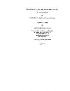
It is clear that the best performance was obtained for the bicriterial dual controller. Attained mean and variance of the criterion have lower values. Utilization of the GS estimator has positive influence for control quality as it is evident from the lower part of the Table 1. The values of the criterion are improved for all four cases. That is confirmed for the IDC and the BDC control in the Figure 1 as well. 50
Vˆ1
(a) 0
0
20
40
60
80
100
50
Vˆ1
(b) 0
0
20
40
60
80
100
50
Vˆ1
(c) 0
0
20
40
60
80
100
50
Vˆ1
(d) 0
0
20
40 60 Trial number
80
100
Fig 1. Obtained values of Vˆ1 for Monte Carlo simulation for chosen regulators and estimators: (a)IDCEKF , (b)BDCEKF , (c)IDCGS , (d)BDCGS . It is suitable to note that even different values of the parameters nf , ng, reference signal and magnitude of noise variance ek were tried without any change of obtained results, i.e. the BCD controller always had the best performance. Example 5.2. The system with three regimes (Fabri and Kadirkamanathan, 2001) is assumed: −1.5yk−1 yk−2 + 0.35 sin(yk−1 +yk−2 ); g1 = 5, f1 = 2 +y 2 1+yk−1 k−2 2.5yk−1 yk−2 f2 = ; g2 = 1, 2 2 1 + yk−1 + yk−2 1.5yk−1 yk−2 f3 = +0.35 cos(yk−1 +yk−2 ); g3 = 3. 2 +y 2 1+yk−1 k−2 The regimes are activated during the time intervals shown in the Table 2. The parameters of model nf , ng are chosen the same as in the first example. Initial values of
REFERENCES
Table 2. The mode activity Mode 1 2 3
Intervals of activity [k] h0, 400), (860, 1140), (1700, 2000i h400, 580), (1420, 1700i h580, 860i, h1140, 1420i
the parameters Θ0 are generated from uniform distribution within the interval h−1, 1i. Number of terms in the GS is set to N0|−1 = 3. Additive noise vk is chosen as sum of two Gaussian distributions, which should model possible high changes of the parameters values during changing of regimes: p(vk ) = 0.997N {vk : 0, 0.0001I} + 0.003N {vk : 0, 0.01I}. Reference signal is set the same as in the first example and the sampling period is set to T = 0.05 sec. Criterion is set as mean of sums of square errors of reference and r system output yki , y , respectively over 100 trials: P100P2000 ki 1 r 2 ˆ V2= 100 i=1 k=1 (yki −yki ) . Table 3. Influence of choice of regulator and estimation method for quality of control system Vˆ2
CEEKF
CAEKF
IDCEKF
BDCEKF
2.3 · 104
7.5 · 104
1.7 · 104
1.4 · 104
109
1011
109
4.3 · 108
cov(Vˆ2 )
2.1 ·
CEGS
CAGS
IDCGS
BDCGS
Vˆ2 cov(Vˆ2 )
1.4 · 103 4·107
544.4 2.3·107
89.3 4.8·104
70.5 7.9·103
1.2 ·
1.3 ·
Influence of choice of control system and estimator on control performance for a more complex system with abruptly changing dynamics is shown in the Table 3. The more sophisticated GS estimator brings significantly better results than the commonly used EKF which can not realize changes of the system dynamics. The bicriterial dual controller brings the best results compared to the others controllers. 6. CONCLUSION The bicriterial dual controller for t-variant nonlinear stochastic systems was presented. The system is given by the multilayer perceptron network. The estimation model is designed and parameters are estimated by the nonlinear filtering Gaussian sum method. The proposed adaptive controller has computational demands comparable with caution control but with dual control ability. The designed approach is useful for abruptly changing systems as well. ACKNOWLEDGEMENT The work was supported by the Ministry of Education, Youth and Sports of the Czech Republic, project No. MSM 235200004 and by the Grant Agency of the Czech Republic, project GACR 102/05/2075.
Alspach, D. L. and H. W. Sorenson (1972). Nonlinear Bayessian estimation using Gaussian sum approximations. IEEE Transactions on Automatic Control, AC-17(4), 439–448. Chen, Fu-Chuang and Hassan K. Khalil (1995). Adaptive control of a class of nonlinear discrete-time systems using neural networks. IEEE Trans. on AC, 40(5), 791–801. de Freitas, J.F.G., M. Niranjan, A. H. Gee and A. Doucet (2000). Sequential Monte Carlo methods to train neural network models. Neural Computation, 12, 955–993. Fabri, Simon G. and Visakan Kadirkamanathan (2001). Functional Adaptive Control: An Intelligent Systems Approach. Springer-Verlag. Fel’dbaum, A. A. (1965). Optimal Control Systems. Academic Press, New York. Filatov, N. M., H. Unbehauen and U. Keuchel (1997). Dual pole-placement controller with direct adaptation. Automatica, 33(1), 113– 117. Maitelli, A. L. and T. Yoneyama (1994). A twostage suboptimal controller for stochastic systems using approximate moments. Automatica, 30(12), 1949–1954. Milito, R., C. S. Padilla, R. A. Padilla and D. Cadorin (1982). An inovations approach to dual control. IEEE Transactions on Automatic Control, AC-27(1), 133–137. Nørgaard, Magnus, O.E. Ravn, N.K. Poulsen and L.K. Hansen (2000). Neural Networks for Modelling and Control of Dynamic Systems. Springer-Verlag. ˇ Simandl, M. (1996). State estimation for nonGaussian models. In: Preprints of the 13th World Congress, IFAC International Federation of Automatic Control. Vol. H. Elsevier Science. San Francisco, USA. pp. 463–468. ˇ Simandl, M. and J. Kr´alovec (2000). Filtering, Prediction and Smoothing with Gaussian sum representation. In: Preprints of Symposium on System Identification. IFAC. Elsevier Science. Santa Barbara, California, USA. ˇ Simandl, M. and M. Fl´ıdr (2001). Bicriterial dual control for stochastic systems with unknown variable parameters. Preprints of the 5th IFAC Symposium on Nonlinear Control Systems. NOLCOS’01, St. Petersburg, Russia. ˇ Simandl, M., P. Hering and L. Kr´al (2004). Identification of nonlinear non-Gaussian systems by neural networks. Preprints of IFAC Symposium on Nonlinear Control Systems. NOLCOS’04, Stuttgart, Germany. Tse, E., Y. Bar-Shalom and L. Meier (1973). Wide-sense adaptive dual control for nonlinear stochastic systems. IEEE Transaction on Automatic Control, AC-18(2), 98–108.