European Transport \ Trasporti Europei (2012) Issue 52, Paper N° 1, ISSN 1825-3997
Neural network based vehicle-following model for mixed traffic conditions Tom V. Mathew, K.V.R. Ravishankar# Transportation Systems Engineering, Department of Civil Engineering Indian Institute of Technology Bombay, Mumbai-400 076, India
Abstract Car-following behaviour is well studied and analyzed in the last fifty years for homogeneous traffic. However in the mixed traffic, following behaviour is found to vary based on type of lead and following vehicles. In this study, a neural network based model is proposed to predict the following behaviour for different lead and following vehicle-type combinations. Performance of the model is studied using data collected for six vehicle-type combinations. A multi-layer feed-forward back propagation network is used to predict vehicle-type dependent following behaviour by incorporating the vehicle- type as input into the model. The neural network model is then integrated into a simulation program to study the macroscopic behaviour of the model. Performance of the proposed neural network model is compared with the conventional Gipps‟ model at microscopic and macroscopic level. This study prompts the need for considering vehicle-type dependent following behaviour and ability of neural networks to model this behaviour in mixed traffic conditions. Keywords: Car-following behaviour, vehicle-type, neural network, macroscopic, simulation.
Introduction Car-following behaviour describes the interaction between two vehicles and is one of the building blocks of traffic simulation tools. Over the past half century, several studies lead to the development of various car-following models such as stimulus-response models, safety distance models, psycho-physical models, optimal velocity models etc. (Brackstone and McDonald, 1999). All these models represent the following behaviour in terms of certain mathematical relationships. In general, most of these models can be represented by one of the following equations:
vtfT f (vtl , vtf , xtl , xtf , p)
(1)
f (v , vt , x , xt , p)
(2)
f t T
a
#
l t
f
l t
f
Corresponding author: Tom V. Mathew (
[email protected]),
[email protected]
1
European Transport \ Trasporti Europei (2012) Issue 52, Paper N° 1, ISSN 1825-3997
where aft+T and vft+T are respectively acceleration and speed of following vehicle at time t+T. vlt and xlt are speed and position of lead vehicle respectively at time t. vft and xft are speed and position of following vehicle respectively at time t and p is a set of parameters for a particular car-following model. Among the several family of carfollowing models, safety distance based models may be more suitable because the effect of vehicle-type clearly reflected on the spacing between the vehicles. Gipps‟ model is one of the widely used safety distance type of model and implemented in various traffic simulation tools such as AIMSUN, MULTISIM, SITRAS etc. (Rakha et al., 2007; Spyropoulou, 2007). Also several studies reported that Gipps‟ model is performing better than other car-following models (Ranjitkar et al., 2004; Punzo and Simonelli, 2005). Gipps‟ model formulation is as follows,
vf vf vtaT vtf 2.5 amax T 1 t 0.025 t , Vn Vn
vtbT
l 2 2 v T t T b b 2 b 2 xtl xtf s vtf T * b 2 2
(3)
(4)
where amax is maximum acceleration rate, Vn is desired speed of vehicle, b is maximum braking rate, b* is assumed braking rate of lead vehicle and s is the effective size of lead vehicle, that is, physical length plus a margin into which the following vehicle is not willing to intrude. When the first condition given by equation 3 is applicable for a substantial proportion of vehicles, free flow traffic exists, whereas the second condition given by equation 4 is applicable for almost all vehicles, congested flow exists. Gipps (1981) proved that when the safety reaction time θ is equal to T/2 and the willingness of the preceding driver to brake hard had not been under estimated, a vehicle traveling at a safe speed would be able to maintain a safe speed and distance indefinitely. The speed update of follower is given by
vtfT Min [vtaT , vtbT ].
(5)
Typical mixed traffic consists of vehicles like passenger car, two wheelers, autorickshaws, light commercial vehicles, buses and trucks. These vehicles significantly vary in the static characteristics (like length, width and size) and dynamic characteristics (like acceleration/deceleration and maximum speed). These differences may influence the following behaviour. For example, the behaviour of a passenger car following a bus is different from the behaviour of a bus following a passenger car. In the former case, driver will have restricted field of vision ahead and is constrained by the lesser acceleration and deceleration capabilities of lead vehicle. Further, recent studies reported the influence of vehicle-type on following behaviour (Brackstone et al., 2009; Ye and Zhang, 2009). Sayer et al. (2000) studied the effect of lead vehicle size (passenger car and light truck) on drivers‟ gap maintenance. Another study observed that trucks are appreciably more conservative than cars as they maintain higher headways (Punzo and Tripodi, 2007). Brackstone et al. (2009) reported that following headway changes according to the type of the following vehicle. Another study on different combinations of lead and following vehicles (car-truck, truck-car, truck-truck,
2
European Transport \ Trasporti Europei (2012) Issue 52, Paper N° 1, ISSN 1825-3997
and car-car) identified qualitative difference in the vehicle-type-specific headway (Ye and Zhang, 2009). These studies clearly indicate the existence of distinct driving behaviour which depends on the vehicle-type. These characteristic differences may greatly affect the car-following process and it may not possible to quantify the vehicletype effect on following behaviour. In order to represent the complex relationship between various vehicle-types, application of a more sophisticated approach such as neural networks can be explored. The neural network models are able to model complex behaviour of a system by identifying the influencing variables and the associated dependent variables without explicitly specifying the mathematical relations between them (Basu et al., 2006). Several studies explored the neural network approach to model car-following behaviour (Hongfei et al., 2003; Wang et al., 2006; Panwai and Dia, 2007). However, these models studied only the behaviour of passenger car following another passenger car. The present study is an attempt to model the vehicle-type dependent following behaviour using neural networks by considering the vehicle-type also as an input. Performance of the proposed neural network model is compared with Gipps‟ model at microscopic and macroscopic level. The contribution of this study is development of a neural network architecture to model the complex driving behaviour under mixed traffic conditions by explicitly considering vehicle-type dependent parameters. The proposed neural network architecture, data collection, implementation, and the results are discussed in the following sections. Neural network model for car-following behaviour Neural network resembles the biological network of the human brain (Heykin, 1994). In a neural network, nodes or neurons are arranged in layers, beginning with an input layer, and ending with the final output layer with a hidden layer in between. Each hidden layer will be having more than one node passing information from the input layer to the output layer. The nodes in one layer are connected to nodes in the next layer and strength of these connections are measured by connection weights. Each node in a layer receives the weighted inputs from the previous layer, converts the weighted sum of the inputs to a single output using an activation function. The connection weights between nodes are optimized through training to produce outputs closest to the measured values. The most commonly used network is a feed-forward network. A multi-layer feed-forward network with back propagation is used in the present study. A feed-forward back propagation neural network is the most commonly used network and the working principle of this network is as follows. First, the effect of the input is passed forward through the network, then the error between targets and predicted output is estimated at output layers, and then propagated back towards the input layer through each hidden node to adjust the connection weight. One complete forward and backward process is known as an iteration (or epoch). This process is repeated until the error between the predicted and measured values falls below a pre-specified error goal or until the number of epochs reaches a pre-determined maximum value. A multi-layer feed-forward network will have one or more hidden layers between the input and output layers. Each hidden layer consists of number of nodes passing information from the input layer to the output layer, and vice-versa in the case of a back propagation network. The proposed architecture of neural network model for predicting the vehicle-type dependent following behaviour is described in the next sub-section.
3
European Transport \ Trasporti Europei (2012) Issue 52, Paper N° 1, ISSN 1825-3997
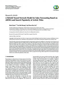
Neural network architecture Traditional car-following models like Gipps‟ models predict the following vehicle speed based on lead vehicle speed and relative distance between vehicles. To model this following behaviour in a neural network requires two inputs namely lead vehicle speed and space headway between vehicles and following vehicle speed as the output. Accordingly a feed-forward back propagation neural network architecture is proposed as shown in Figure 1a. Although explicit vehicle-type is not specified, the space headway may act as a proxy to the vehicle-type. This architecture is referred as NN 1 (Neural network 1) model in this paper. A better alternative of predicting the vehicletype dependent following behaviour is to explicitly specify the vehicle-type in the model itself. This can be done in two ways: first by considering the vehicle-type combination (that is lead-following vehicle-type combination) as an input and the second by considering lead vehicle-type and following vehicle-type as separate inputs. The former architecture has three inputs namely lead vehicle speed, space headway, and lead-following vehicle-type combination. This architecture is shown in Figure 1b and referred as NN 2 model in this paper. The latter architecture has four inputs namely lead vehicle speed, space headway, lead vehicle-type, and following vehicle-type This architecture is shown in Figure 1c and referred as NN 3 model. The NN 2 architecture models the vehicle-type dependent following behaviour based on the characteristic differences between the vehicle-type combinations such as three wheeled auto-rickshaw following a passenger car, bus following a passenger car etc. In the case of NN 3 architecture, following behaviour is predicted based on the type of lead and following vehicle-types. The basic hypothesis of these architectures is that the inclusion of vehicle-type will improve the prediction of following behaviour in mixed traffic conditions. Evaluation For evaluating the performance of neural network model, difference between the predicted and measured values of following vehicle speed is analyzed. This difference can be measured through any of the following error values: mean square error, root mean square error, and Theil‟s error values. However, Theil‟s error measure provides additional insights on the nature of source of error in the models. The mean square error (em) is used to measure the performance of a training process and is given as the average sum of the squares of the difference between measured output and neural network predicted output values. The mean square error is defined as em
1 N
N
(y
o
i 1
ym ) 2 .
(6)
where yo and ym are observed and predicted values respectively and N is number of observations. Theil (1966) introduced an accurate and sensitive error measure known as Theil‟s error value (U) and is given as, N
1 N
U 1 N
(y i 1
N
(y i 1
o
o
ym ) 2 1 N
)2
4
.
N
(y i 1
m
)2
(7)
European Transport \ Trasporti Europei (2012) Issue 52, Paper N° 1, ISSN 1825-3997
Theil‟s value is between 0 and 1, with a value of 0 indicating a perfect fit. Theil‟s error value can be decomposed into three proportions namely Theil‟s bias (Um), variance (Us), and covariance (Uc), which provides additional insights on the nature of source of error (Pindyck and Rubinfeld, 1998).
Fig. 1. Three neural network architectures with different inputs for predicting the vehicle-type dependent following behaviour
These are useful for breaking down the simulation error into its characteristic sources. For a perfect match of model results to field values, Theil‟s bias and variance should be as close as possible to zero and covariance should be close to 1. The greatest advantage of using Theil‟s error measure is that it gives an error measure independent of magnitude of the parameter. Mean square error is used in the neural network training
5
European Transport \ Trasporti Europei (2012) Issue 52, Paper N° 1, ISSN 1825-3997
phase and Theil‟s error measure is used in testing and validation phase. A genetic algorithm (GA) based optimization technique is used to calibrate the Gipps‟ carfollowing parameters. GA based optimization techniques are very effective, widely used and can be easily integrated with car-following models to calibrate parameters (Ranjitkar et al., 2004). Theil‟s error is used as objective function in calibrating the Gipps‟ model parameters. The calibration of Gipps‟ model is performed separately for each vehicle-type combination. The parameter values which yield minimum Theil‟s error are treated as calibrated parameter values. The calibrated parameters are used to analyze the performance of the Gipps‟ model in testing and validation phases. The performance of Gipps‟ model and neural network model is analyzed at microscopic level by comparing the observed speed values with the model values. In order to study the performance of the network at macroscopic level, neural network is integrated into a simulation program and the speed-flow relationship is analyzed and compared with field and Gipps‟ model values. A detailed description of the data collection procedure is presented in the next section followed by neural network implementation. Data collection Two major urban arterials of Mumbai in India, are selected for data collection. A 5.6 km long straight section on Eastern express highway and 4.9 km stretch on Western express highway in Mumbai are selected. These sections are six lane divided urban highways with typical traffic volumes ranging from 833 to 1066 vehicles/hr/lane. These stretches are continuous sections with no major intersections and represent a typical urban traffic. Data was collected using vehicles equipped with Global positioning system (GPS) receivers Experiments were conducted with six combination of vehicles comprising of passenger car (length 4.7 m), three wheeled auto-rickshaw (length 2.6 m), and bus (length 9.4 m). The six combinations are namely, passenger car following another passenger car (C-C), three wheeled auto-rickshaw following a passenger car (C-A), passenger car following a three wheeled auto-rickshaw (A-C), three wheeled autorickshaw following another three wheeled auto-rickshaw (A-A), passenger car following a bus (B-C) and bus following a passenger car (C-B). As the selected stretches are multi-lane highways, drivers of vehicles were instructed to adhere to a particular lane during the experiment. With the help of beacon receiver, the real time differentially corrected GPS data was recorded. Data was obtained from a series of experiments carried out along the selected stretches under real traffic conditions during February to March, 2008. As the car-following behaviour may change in rainy conditions and at night time due to less visibility, experiments were conducted on sunny days and during peak and off-peak time. Preliminary surveys were conducted for assessing the satellite availability and traffic characteristics. Leading vehicle driver was asked to follow the traffic stream and the following vehicle driver to follow the lead vehicle without overtaking and maintaining a desired safe gap. Drivers selected for the data collection are regular drivers and were not aware of the objectives of the study. They were in the age group of 25 to 30 years and data was collected from four different drivers for each vehicle-type combination. Data sets containing lane changing or extrusion of vehicles between lead and following vehicles were excluded. Characteristics of the data set considered for analysis are shown in Table 1.
6
European Transport \ Trasporti Europei (2012) Issue 52, Paper N° 1, ISSN 1825-3997
Table 1: Car-following data sets.
Leader-Follower C-C C-A A-C A-A B-C C-B Duration Training andTesting 1075 1960 1370 1915 1275 1045 (seconds) Validation 255 280 395 360 305 230 key: C-C: passenger car following a passenger car; C-A: three wheeled auto-rickshaw following a passenger car; A-C: passenger car following a three wheeled auto-rickshaw;A-A: three wheeled autorickshaw following a three wheeled auto-rickshaw; B-C: passenger car following a bus; C-B: bus following a passenger car;
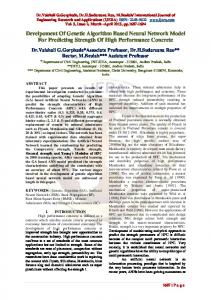
After filtering the data for satellite unavailability that is if the data is unavailable for the lead or following vehicle for a particular duration of time, then that data was excluded from analysis. Also care is taken that data does not show any abnormalities like very high acceleration/deceleration values. A total of 144 minutes of data was selected from eastern express highway and used for training and testing of network. Another data for 30 minutes was obtained from western express highway and used for validating the trained network. Vehicle-type dependent following behaviour An examination of space headway (distance between the rear of the lead vehicle to the front of following vehicle) for the different vehicle-type combinations showed a vehicle-type dependent behaviour. The cumulative distribution of space headway for the six vehicle-type combinations is shown in Figure 2.
Fig 2. Cumulative frequency distribution of space headway for different vehicle-type combinations key: C-C: passenger car following a passenger car; C-A: three wheeled auto-rickshaw following a passenger car; A-C: passenger car following a three wheeled auto-rickshaw;A-A: three wheeled autorickshaw following a three wheeled auto-rickshaw; B-C: passenger car following a bus; C-B: bus following a passenger car;
7
European Transport \ Trasporti Europei (2012) Issue 52, Paper N° 1, ISSN 1825-3997
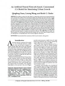
It was observed that three wheeled auto-rickshaw followed another three wheeled autorickshaw at a closer spacing, whereas bus followed a passenger car at a higher spacing. Due to the higher maneuverability and smaller size of three wheeled auto-rickshaw vehicles, they maintained lesser following distance. However, due to the raised view of the driver in the case of bus following a passenger car, driver may anticipate the traffic and maintain higher gaps. Hence the gap maintained by a following driver depends on the size and characteristics of vehicle-type. For example, small sized vehicles can maneuver easily in a traffic stream and may follow the lead vehicle at a lesser spacing compared to large vehicles. Space headway values were in the range of 2 m to 24 m for the auto-rickshaw following another auto-rickshaw (A-A) combination, where as for the bus following passenger car combination (C-B), these values were in the range of 6 m to 55 m. As the space headway maintained by a vehicle is going to depend on the speed of the vehicles, analysis is conducted for various speed categories (multiples of 5 m/s). Mean and standard deviation of space headway for different vehicle-type combinations at different speed distributions is shown in Figure 3. It can be seen from this figure that
Fig 3. Mean and standard deviation of space headway for various vehicle-type combinations at different speed distributions key: C-C: passenger car following a passenger car; C-A: three wheeled auto-rickshaw following a passenger car; A-C: passenger car following a three wheeled auto-rickshaw;A-A: three wheeled autorickshaw following a three wheeled auto-rickshaw; B-C: passenger car following a bus; C-B: bus following a passenger car;
the space headway distribution varies significantly with the vehicle-type for almost all speed ranges. However, the variation in space headway is more predominant in the case of bus following a passenger car across the different speed distributions. Thus vehicletype has a considerable influence on the following behaviour. These results suggest that in addition to driver heterogeneity, vehicle-type heterogeneity should be considered in predicting the following behaviour particularly in mixed traffic conditions. This type of distinct behaviour is to be properly modeled in traffic simulation tools and neural network approach may be one of the options to describe this complex relationship. Implementation and Results In a neural network, learning process which extracts information from the input data is an important step. Approximately, seventy percent of data collected on eastern express highway is selected for training and remaining data for testing of the network.
8
European Transport \ Trasporti Europei (2012) Issue 52, Paper N° 1, ISSN 1825-3997
Validation of the network is accomplished using data collected on another arterial western express highway. The „newff‟ function available in MATLAB neural network tool box is used to create the multi-layer feed-forward back propagation network (MathworksInc, 2008). In order to ensure that all variables receive equal attention during the training process, inputs and targets are normalized between 0 to 1 before feeding into the network. For representing the lead and following vehicle-type combination as an input into the NN 2 and NN 3 architectures, each vehicle-type combination is given a value in the range 0 to 1. To ensure that over training does not occur and the network is well trained, the following criteria are set during training process. The training process is continued till the maximum number of epochs is reached or an acceptable error level is attained. The maximum number of iterations (or epochs) is set to 1000. The threshold value for the mean square error is set to 10−8 during the training process. The philosophy behind this is to let the network train until it basically cannot extract any information from the training data. The minimum performance gradient is set to 10-10. The termination of training process at this level is justified because the network performance does not improve even if the training continues. In order to overcome the criteria of initial weights and stopping criteria, the training is repeated for a specific network architecture and the result with lesser error is considered as optimal network. Several back propagation algorithms were tried and it was found that Levenberg-Marquardt back propagation algorithm best fits the present problem and was reported to be the fastest convergence algorithm (MathworksInc, 2008). Calibration of the Gipps‟ model was done using the training data and using the calibrated parameters, performance of the Gipps‟ model is analyzed on testing and validation data. Neural network structure optimization The most critical phase of a feed-forward back propagation network is determination of number of hidden layers and number of nodes in each hidden layer. This is generally accomplished through a trial and error procedure with different network structures. A number of network structures are tested by varying the number of hidden layers and neurons in each hidden layer. As discussed earlier, the three network architectures with different inputs were studied for different number of hidden layers and number of nodes in each hidden layer. Performance of the network is analyzed by comparing the Theil‟s error value for different architectures. Theil‟s error (U) and its decomposition values namely Theil‟s bias, variance, and covariance values for the different neural network architectures are given in Table 2. A multi-layer feed-forward back propagation network with 2-2-2-1 architecture (two hidden layers each with two hidden nodes) outperformed other architectures for the NN 1 network. Also, ideal values of Theil‟s bias, variance, and covariance values were observed for this network. Similarly optimal networks for the NN 2 and NN 3 architectures were found by varying the number of hidden layers and number of nodes in each layer. A common observation in these optimal networks is that the use of more than one hidden layer provides a better prediction of following behaviour with fewer neurons in the hidden layers. This result is consistent with a previous study in which the use of more than one hidden layer provides greater flexibility and prediction of complex functions with fewer neurons (Flood and Kartam, 1994). The optimal network structure is used for testing and validation of other vehicletype combinations and discussed below.
9
European Transport \ Trasporti Europei (2012) Issue 52, Paper N° 1, ISSN 1825-3997
Table 2: Sensitivity analysis of different neural network architectures for the passenger car following a passenger car combination
NN architecture Structure 2-2-1 2-4-1 2-6-1 2-2-1-1 2-2-2-1 2-2-3-1 NN1 2-2-4-1 2-1-2-1 2-3-2-1 2-4-2-1 2-5-2-1 2-3-3-1
NN2
3-2-1 3-4-1 3-6-1 3-2-2-1 3-2-3-1 3-2-4-1 3-1-2-1 3-3-2-1 3-4-2-1 3-3-3-1
4-2-1 4-4-1 4-6-1 NN3
4-2-2-1 4-2-3-1 4-2-4-1 4-1-2-1 4-3-2-1 4-4-2-1 4-3-3-1
U 0.0337 0.0335 0.0367 0.1631 0.0332 0.0337 0.1113 0.0334 0.0336 0.0337 0.0453 0.0627
Um 0.0189 0.0151 0.0125 0.5194 0.0119 0.0248 0.3196 0.0182 0.0174 0.0147 0.0012 0.0184
Us 0.1863 0.1863 0.2001 0.4807 0.1764 0.2069 0.3849 0.1983 0.1918 0.2011 0.0994 0.1855
Uc 0.7948 0.7986 0.7873 0.0001 0.8118 0.7683 0.2955 0.7835 0.7908 0.7842 0.8995 0.7592
0.0343 0.0358 0.0363 0.0336 0.0316 0.0436 0.0331 0.0332 0.0337 0.0417 0.0336 0.0336 0.0336 0.0338 0.0338 0.0340 0.0321 0.0410 0.0342 0.0457
0.0198 0.0315 0.0229 0.0284 0.0250 0.0531 0.0213 0.0261 0.0327 0.0368 0.0302 0.0205 0.0325 0.0128 0.0383 0.0151 0.0244 0.0320 0.0099 0.0219
0.1751 0.1848 0.3221 0.1846 0.1700 0.3116 0.1979 0.1711 0.1988 0.2168 0.1877 0.2045 0.1879 0.2292 0.1921 0.1606 0.1701 0.3611 0.2500 0.2781
0.8052 0.7837 0.6550 0.7870 0.8502 0.6353 0.8082 0.8028 0.7685 0.7246 0.7821 0.7750 0.7796 0.7580 0.7695 0.8242 0.8055 0.6069 0.7400 0.6818
Key: NN: Neural network; U: Theil‟s error; Um: Theil bias; Us: Theil variance; Uc: Theil covariance; 2-2-1 Structure represents a feed-forward back propagation network with two inputs, two nodes in the hidden layer, and one output; 2-2-2-1 structure represents two inputs, two hidden layers each with two nodes, and one output;
Performance at microscopic level In order to compare the performance of the optimal neural network architectures, mean and standard deviation of follower speed from neural network output is compared with Gipps‟ model and field values as shown in Table 3. Theil‟s error value is also reported for the three network types and Gipps‟ model in the above table and these results are from the testing phase i.e. considering 30% of data collected from eastern express highway.
10
European Transport \ Trasporti Europei (2012) Issue 52, Paper N° 1, ISSN 1825-3997
Table 3: Comparison of mean and standard deviation of speed and Theil‟s error values for the three neural network architectures among the six vehicle-type combinations from testing results
L-F μ C-C C-A A-C A-A B-C C-B
Field σ
14.1 8.4 9.9 8.7 6.9 6.5
2.8 0.8 1.8 1.6 3.4 3.7
μ
NN1 σ
14.2 8.0 10.3 8.0 6.7 6.1
2.3 0.8 1.6 1.6 3.2 3.3
U
μ
NN2 σ U
μ
NN3 σ U
μ
Gipps σ U
0.033 0.034 0.037 0.032 0.041 0.058
14.1 8.2 10.1 8.4 7.0 6.5
2.3 0.8 1.6 1.6 3.2 3.4
14.2 8.1 10.2 8.3 6.4 6.2
2.4 0.9 1.6 1.6 3.0 3.1
13.7 7.90 10.2 7.90 6.30 6.60
2.9 1.1 1.6 1.9 3.6 3.7
0.031 0.030 0.029 0.029 0.033 0.053
0.032 0.03 0.034 0.032 0.04 0.061
0.039 0.053 0.055 0.078 0.074 0.061
key: μ: NN: Neural network; Mean speed of following vehicle; _: Standard deviation of speed of following vehicle; U: Theil‟s error; C-C: passenger car following a passenger car; C-A: three wheeled auto-rickshaw following a passenger car; A-C: passenger car following a three wheeled auto-rickshaw; AA: three wheeled auto-rickshaw following a three wheeled auto-rickshaw; B-C: passenger car following a bus; C-B: bus following a passenger car;
A comparison of Theil‟s error value for the three networks shows that the NN2 network with three inputs (that is considering lead-follower vehicle-type combination in addition to lead vehicle speed and space headway) is performing better than the other two network types and Gipps‟ model. Mean values of follower speed from NN2 network were quite close with field values for all the vehicle-type combinations. One of the possible reasons can be that when the vehicle-type combination is given as input, neural network tries to capture the distinct behaviour by considering the variation in following behaviour across the combinations. Whereas, in the case of NN3 architecture with four inputs (that is considering lead and follower vehicle-types) is not be able to establish any relation particular to a vehicle-type. Thus considering the vehicle-type combinations as input improves the prediction of vehicle-type dependent following behaviour. Similar observation can be found from the validation results (considering data obtained from western express highway) as shown in Table 4. Table 4: Comparison of mean and standard deviation of speed and Theil‟s error values for the three neural network architectures among the six vehicle-type combinations from validation results
L-F C-C C-A A-C A-A B-C C-B
Field μ σ
Μ
6.7 7.4 8.5 8.8 13.6 11.6
7.0 6.7 8.9 8.0 13.0 11.1
1.5 2.5 2.0 3.2 4.9 1.6
NN1 σ U 1.4 2.1 1.9 2.9 4.7 1.7
μ
NN2 σ U
0.031 6.8 1.3 0.048 7.3 2.3 0.047 8.6 2.0 0.054 8.6 2.7 0.029 13.2 4.4 0.036 11.4 1.6
0.029 0.034 0.040 0.045 0.024 0.027
μ
NN3 σ U
μ
Gipps σ U
6.9 7.1 8.8 8.1 13.1 11.3
1.4 2.3 2.0 2.9 4.8 1.7
6.1 7.6 8.2 9.1 13.4 11.8
1.8 2.6 2.3 3.3 5.2 1.6
0.027 0.037 0.047 0.046 0.028 0.029
0.047 0.051 0.066 0.097 0.044 0.034
key: NN: Neural network; μ: M ean speed of following vehicle; σ : Standard deviation of speed of following vehicle; U: Theil‟s error; C-C: passenger car following a passenger car; C-A: three wheeled auto-rickshaw following a passenger car; A-C: passenger car following a three wheeled auto-rickshaw; AA: three wheeled auto-rickshaw following a three wheeled auto-rickshaw; B-C: passenger car following a bus; C-B: bus following a passenger car;
A comparison of the mean and standard deviation values of follower speed from NN2 neural network with Gipps‟ model suggests that vehicle-type dependent following
11
European Transport \ Trasporti Europei (2012) Issue 52, Paper N° 1, ISSN 1825-3997
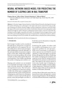
behaviour can be closely represented with neural network models considering the vehicle-type combination as one of the input parameters. The validation error values for the bus following a passenger car combination and passenger car following a bus were less in the validation compared to testing phase. First, it can be observed that mean values of following vehicle speed vary across the vehicle-type combinations indicating the vehicle-type dependent following behaviour. These results suggest that a well trained neural network can be conveniently used for an altogether different data set. The following vehicle speed profile from the three neural network architectures is compared with Gipps‟ model output and field speed profile for the three wheeled auto-rickshaw following another three wheeled auto-rickshaw (A-A) combination and three wheeled auto-rickshaw following a passenger car (C-A) combination as shown in Figure 4.
Fig 4. Comparison of following vehicle speed profile from four layer feed-forward back propagation neural network with Gipps‟ model and field values for the A-A and C-A combinations
It can be observed that the neural network output are in close agreement with field values compared to Gipps‟ model. Among the three neural network architectures studied, the two architectures incorporating vehicle-type (that is NN2 and NN3 neural
12
European Transport \ Trasporti Europei (2012) Issue 52, Paper N° 1, ISSN 1825-3997
network) were able to capture the field behaviour closely. In order to study the performance of neural network model at macroscopic level, a simulation study is conducted as described below. Performance at macroscopic level A single lane simulation study is conducted for a better understanding of the application of neural network model at macroscopic level. This helps in studying the actual application of the model in traffic simulation. The simulation process consisted of the following steps: vehicle generation, vehicle movement and integration of neural network model. The simulation process was developed using c-programming. Traffic simulation models being stochastic in nature, requires randomness. This is accomplished through generating random numbers and subsequently vehicles are generated using negative exponential distribution of headways. As it was observed that NN 2 neural network model is performing better compared to other two neural network models, this network is used in the simulation. Lead vehicle speed, space headway between vehicles, and the lead-following vehicle-type combination is assigned as input to the neural network model. The neural network model gives the following vehicle speed as output which is assigned to the following vehicle and the position of vehicle is updated. This process is continued for the rest of vehicles till the end of simulation period. In the case of simulation using Gipps‟ model, speed update of following vehicle was done as per the calibrated Gipps‟ model parameters. The simulation is conducted for a stretch of 1000 m. Number of runs were conducted to nullify the effect of random numbers and average values of fundamental parameters were obtained for ten runs. Fundamental parameters of traffic: flow, speed and density values are obtained from the middle of stretch (250 m to 750 m) to mitigate any transient nature of traffic flow. As the neural network architecture NN2 is performing comparatively better than other architectures, this architecture is used in the simulation study. The speed-flow estimates from the simulation are plotted and compared with field observations and Gipps‟ model results as shown in Figure 5.
Fig 5. Comparison of speed-flow values from simulation using multi-layer feed-forward back propagation neural network model and Gipps‟ model with field values
13
European Transport \ Trasporti Europei (2012) Issue 52, Paper N° 1, ISSN 1825-3997
The speed-flow relationship from NN2 neural network is closer to the field observations compared to Gipps‟ model. Thus neural network integrated models are able to capture the mixed traffic conditions better than conventional models. Also neural network simulated speed-flow values show a better correlation with field values compared to the values using Gipps‟ car-following model. This shows that a neural network well trained for different vehicle-type combinations can be used for simulating the mixed traffic environment and shows the potential of this technique to be used in simulation models. Conclusion In this study, vehicle-type dependent following behaviour of different lead and following vehicle-type combinations is modeled using neural network approach and compared with conventional Gipps‟ car-following model performance. A multi-layer feed-forward back propagation network with different inputs were used to predict the following behaviour. Three different neural network architectures with number of inputs were studied and these architectures consist of lead-following vehicle-type/types in addition to the lead vehicle speed and space headway as inputs to the neural network. Data was collected for the six lead and following vehicle-type combinations comprising of passenger car, three wheeled auto-rickshaw, and bus. Performance of the neural network model is studied at microscopic level by comparing the follower speed with field values and at macroscopic level by comparing the speed-flow relationship. Among the three neural network architectures studied, three input neural network considering explicit vehicle-type combination as one of the inputs performed better than other network architectures and conventional Gipps‟ model. At macroscopic level, simulated speed-flow relationship from neural network model is close to the field behaviour compared to Gipps‟ model. This study thus demonstrates the efficacy of the neural network architecture to accurately model the vehicle-type dependent following behaviour significantly better than conventional model. This study has wider implications in simulation tools aiming at modeling complex traffic systems.
References Basu, D., Maitra, S. R., Maitra, B. (2006). “Modelling passenger car equivalency at an urban midblock using stream speed as measure of equivalence.” European Transport/ Trasporti Europei, 34, pp. 75–87. Brackstone, M., McDonald, M. (1999). “Car-following: A historical review.” Transportation Research Part F: Traffic Psychology and Behaviour, 2(4), pp. 181–196. Brackstone, M., Waterson, B., McDonald, M. (2009). “Determinants of following headway in congested traffic.” Transportation Research Part F: Traffic Psychology and Behaviour, 12(2), pp. 131–142. Flood, I. Kartam, N. (1994). “Neural networks in civil engineering. : Principles and understanding.” Journal of Computing in Civil Engineering, ASCE, 8(2), pp. 131–148. Gipps, P. G. (1981). “Behavioural car-following model for computer simulation.” Transportation Research, Part B: Methodological, 15 B(2), pp. 105–111. Heykin, S. (1994). Neural Networks: A Comprehensive Foundation. Mac-Millan, New York.
14
European Transport \ Trasporti Europei (2012) Issue 52, Paper N° 1, ISSN 1825-3997
Hongfei, J., Zhicai, J., Anning, N. (12-15 Oct. 2003). “Develop a car-following Model using data collected by ”five-wheel system”.” Intelligent Transportation Systems, 2003. Proceedings. 2003 IEEE, 1, pp. 346–351 vol.1. MathworksInc (2008). “Matlab neural network toolbox user‟s guide.” Natick, USA.Panwai, S. and Dia, H. (2007). “Neural agent car-following models.” IEEE Transactions on Intelligent Transportation Systems, 8(1), pp. 60–70. Punzo, V., Simonelli, F. (2005). “Analysis and comparison of microscopic traffic Flow models with real traffic microscopic data.” Transportation Research Record 1934, Journal of the Transportation Research Board, Washington D.C., pp. 53– 63. Punzo, V., Tripodi, A. (2007). “Steady-state solutions and multiclass calibration of gipps microscopic traffic flow model.” Transportation Research Record 1999, Journal of the Transportation Research Board, Washington D.C., pp. 104–114. Rakha, H., Pecker, C. C., Cybis, H. B. B. (2007). “Calibration procedure for gipps carfollowing model.” Transportation Research Record 1999, Journal of the Transportation Research Board, Washington D.C., pp. 115–127. Ranjitkar, P., Nakatsuji, T., Asano, M. (2004). “Calibration and validation of microscopic traffic flow models using rtk gps data.” Proceedings of the International Conference on Applications of Advanced Technologies in Transportation Engineering, Vol. 144, ASCE. pp. 395–400. Sayer, J. R., Mefford, M. L., Huang, R. (2000). “The effect of lead-vehicle size on Driver following behaviour.” Report No. UMTRI-2000-15, The University of Michigan Transportation Research Institute, U.S.A, Report no. UMTRI- pp. 200015. Spyropoulou, I. (2007). “Modelling a signal controlled traffic stream using cellular automata.” Transportation Research Part C Emerging Technologies, 15(3), pp. 175–190. Theil, H. (1966). Applied Economic Forecasting. North Holland Publishing Company, Netherlands. Wang, L., Liu, X., Zhong, X. (2006). “A car-following model based on artificial neural networks in urban expressway sections.” 85th TRB Annual Meeting, Transportation Research Board, National Research Council, Washington D.C. Ye, F.. Zhang, Y. (2009). “Vehicle-type-specific headway analysis using freeway Traffic data, presented at the 88th annual meeting of the transportation research board.” Number Report no.:09-2997, Washington D.C.
15