Neural Networks for Signal Processing

O N THE USE OF A P R U N I N G PRIOR FOR NEURAL NETWORKS Cyril Goutte* Department of Mathematical Modeling - Bygn. 349 Technical University of Denmark DK-2800 Lyngby, Denmark Phone: $45 4525 5738 Fax: $45 4288 0117 E-mail: gout [email protected]

Abstract. We adress the problem of using a regularization prior that prunes unnecessary weights in a neural network architecture. This prior provides a convenient alternative to traditional weight-decay. Two examples are studied to support this method and illustrate its use. First we use the sunspots benchmark problem as an example of time series processing. Then we adress the problem of system identification on a small artificial system.

OVERVIEW It is well known that the use of a regularization term during optimization improves the general accuracy of the model obtained. In the case of neural networks, regularization is most often used through the addition of a weight-decay term to the cost function in order to improve the generalization abilities of the solution [5].Other methods for improving these abilities include pruning, a.long the lines of OBD [6]. These techniques have been applied to a wide variety of problems, including time series and system identification. In this paper, we analyse the use of another regularization term, due to [Ill, which is supposed to have some pruning capabilities [ 3 ] .After presenting this technique, we illustrate its use on both time series-the well known sunspots benchmark-and a system identification problem. The results obtained tend to illustrate in a convincing way the effect of this *visiting student, 1995-1996. Permanent adress: Equipe connexionniste - LAFORIA, UniversitC Paris VI, 4 place Jussieu, 75252 Paris Cedex 05, France. E-mail: goutteOlaforia.ibp.fr

0-7803-3550-3/96$5.00@ 1996

52

Authorized licensed use limited to: Danmarks Tekniske Informationscenter. Downloaded on July 14,2010 at 11:29:10 UTC from IEEE Xplore. Restrictions apply.

prior on 1e;sriiing.

PRUNING PRIOR Neural networks have been applied extensively to many kinds of problems. Among those, we will here consider time series modelling and system identification, which constitute important applications of signal processing. . The basic neural network model we will consider here is the multi-layered perceptrons model, with one hidden layer. This neural network model, having n~ inputs, 7 1 hidden ~ units and one output', contains p = (711 2) n~ 1 parameters. We will write these parameters wji for the weight going from input i to the hidden cell j , and Wj for the weight goi.ng from hidden cell j to the output. The response of the network to an input 2 = [ 2 i ] l , , , , , nis: I

+

where 12 is a-usually biases of the model.

sigmoid-Lransfer

function. W, and the

tujo

+

are the

The parameter identification procedure ltnowii as training is performed by optimizing a cost function including two terms:

C ( w ) = S(2u)

+ @qw)

(2)

where the first part of the right-hand side, S ( w ) , is the usual average quadra1 , that is: S(w) = tic cost calculated on N input-output examples ( ~ ( ~ Y(~)),

( ~ (~ f1w

(d')))2 . A regularization

term R(w) has been added to S(w). This is known as formal regularization [ 2 ] ,the effect of which is weighed by parameter I . An optimal value of exists, for which the generalization abilities of the solution that minimizes (2) are superior to those of the unregularized solution-and possibly equal when = 0. Another way to improve generalization, is to use pruning algorithms to get rid of unnecessary parameters. Among pruning methods fix neural networks, the most common are OBD [6] and OBS [4]. These methods physicaly decrease the capacity of the model in order to limit over-fitting,. They go by the name of structural regularization. In the case of weight-decay, the additional term coriresponds to a gaussian prior on the weight distribution. We will here address the use of a new kind of regularization function, introduced by [ll].It corresponds to a Laplace prior 'We will consider the case of one output, as it is all we need for the applications we consider here. It should be understood, though, that this is not a limitation of the model, and by no means of the prior, but only a case-specific setting driven by practical considerations.

53


on the weights, and leads to the following expression for the regularized cost:

where W is the set of weights on which we regularize, and is a positive regularization parameter. Interesting insight into the effect of this new prior ca.n be obtained by stating the obvious: at the minimum W of (3), the first derivatives are 0. For any non-zero weight, the first derivative of the quadratic cost reads:

This means that the value of any nun zero parameter is found at a point where the sensitivity of the data misfit to this parameter is in accordance with (4). If this is not possible (i.e. the sensitivity is nowhere that high), the parameter is forced to 0 and pruned out of the network. We have studied this prior in [3] and analysed its joint formal and structural regularization effect on a simple case. On a practical aspect, the fact that, the regularization function is not analytical in 0 might be seen as possibly causing problems. In order to analyse that particular point, we have compared results obtained with the absolute value to those obtained with an analytical approximation:

re(.) = t l n (2ch

(:))

(5)

that converges uniformly towards 1 . I. Results obtained using (5) have been slightly but consistently worse than wit,h the standard absolute value. The reason for this is not so clear. It is our understanding that for high values of 6, the convergence should be similar to that of the standard absolute va,lue, but is hampered by numerical problems due the calculation of ch (z/t). On the other hand, for low values of E , the zone in weight space where the derivative of (5) i s close to zero is rather large, which suppresses the effect of the regularization before the weights are significantly close to 0.

TIME SERIES PROCESSING In order to illustxate the use of the pruning prior for time series processing, we chose the well known sunspots data. These have been historicaly the first time series studied using an aut,oregressive model [12]. They have been established since [IO] as one of the benchmarks for time series prediction algorithms using neural networks. This series is a yearly record of average sunspot activity. It has been recorded since 1700, and displays a cyclic pattern with maxima. The time between these ranges from 7 to 17 years, with a median of 11 years. In accordance with previous work, we attempt to predict one value using the twelve previous ones, leading to a network with 12 input units and one output

54


First and second layer weight values

Neural Network Y(t-l)\

L -20

20

2

r

40 60 Input-to-hidden

80 100 weight no.

120

I

I -2L-3

4 6 8 Hidden-to-output weight no.

10

Input layer

Hidden layer

Output layer

Figure 1: Top-left: input-to-hidden weights, by hidden unit,. Every hidden unit has 13 incoming connections: weights 1Gl3 go to HU 1, weights 14-26 t o HU 2, etc. Bottom-left: hidden-to-output weights. Right: the network. Dotted lines correspond t o connections that are one order of magnitude lower thein those in solid line. A vertical line through a cell corresponds t o an active threshold.

unit. The available data constitutes 268 input-output pairs which are split into three sets. In the training set, we try to predict activities from 1712 to 1920, amounting to 209 examples, the test set uses data from 1921 to 1955 (35 pairs), and the validation set runs from 1956 to 1979 (24 examples). Performance is measured in terms of average relative variance (arv), which is the ratio between the average squared error of the model and the variance of the data2 The model we used is a 12-10-1 neural network, containing 141 paraineters, which can be considered as highly over-paramet*rized compared to the 209 data in the training set. Training is performed by minimizing the cost function (3) as mentionned above. The optimization t#echniqueis a standard conjugate gradient, similar to [8], implemented under .the SN simulation software, froin Neuristique [l].The regularization parameter is set with the help of the test set, by chosing the value of X that minimizes the test error, and t,he results are evaluated on the validation set. This scheme is not very satisfying, but has been adopted because it makes use of the 3 available sets in a manner similar to that of [lo]. 21t should be noted here that the more widely used definition scales by the overall variance of the data. This gives artificially high values of the error on the validation set, where the intrinsic data variance is around twice as high as in the other sets. A more “proper” definitionof the arv quantity would relate the error of the model and the variance (yk - f ( ~ k ) /) ~ (y, - (yk)kEs)2. of the data calculated on the same set In order to ease comparison with other papers, we will stick to the widely used definition. The proper numbers can be obtained by multiplying the given. values by 1.277, 0.903 and 0.496 for the training, test and validation sets respectively.

E,,,

55


log abolute value of input-to-hidden weights

L-ddId 4

-2

0

lorlwl

Figure 2: Left: magnitude of the input-to-hidden weights. Notice the logarithmic y-axes. Right: distribution of the log absolute value of the weights. Notice the two modes corresponding to the pruned and not pruned weights.

Results The parameters of one of the networks we obtained are displayed on figure 1. It can be seen that in the course of the learning procedure, 6 of the hidden units have been disabled, and effectively pruned. Some of the input connections of the remaining hidden units have also been driven to 0 (e.g. in the third hidden unit). The solution displayed here is typical of those we obtained: 3 units perform most of the work, with one (sometimes two) additional units contributing to a lesser extent. Concerning the inputs, the biggest contributions come from the first units, one middle unit (t - 8 here) and the last two units. This pattern has already been observed by [9] using a completely different method. Figure 2 corroborates this by displaying the distribution of the weights. On the left panel, the magnitude plot shows that input weights of the sa,me network have been more or less clustered in two categories: roughly, the active weights are greater than when the rest are gathered below l o e 4 . Again, we see that six hidden units have been effectively discarded. On the right, the empirical distribution of the absolute values of the weights of 10 networks trained with t,he pruning prior. With a logarithmic X-axis, it clearly displays two modes, one corresponding t o the pruned parameters, and the other to those that are still in use. Apart from its illustrative purpose, this provides a. way of empiricaly counting the number of effective parameters. This number can be used t o obtain an algebraic estimat,e of the generalization error. This leads us to discussing the empirical distribution of the weights. A natural idea would be tlo test this empirical distribution against the Laplace distribution that we used as a prior. I t should be clear from the plots presented here that the solution parameters do not follow a Laplace distribution, and that is to be expected. As Bayesians are well aware, one should indeed not confuse the probability of the weights (the posterior, i.e. regularized cost) with the assumption on their distribution (the prior, i.e. the regularization

56


Model/arv Linear Weigend & al. [lo] Svarer & al. [9] Pruning prior

Train (1712-1920) 0.131 0.082 0.090 f 0.001 0.082 f 0.001

Test (1921-1955) 0.128 0.086 0.082 f 0.007 0.082 f 0.002

Valid at ion (1956-1979) 0.36 0.35 0.35 f 0.05 0.357 5 0.013

Table 1: Comparison of the results obtained using different methods. The linear model includes an intercept. The results reported for Svarer ib al. are averaged over 9 retrained networks; for the pruning prior we averaged over’ 10 network solutions. functional) Of higher interest is the consideration of the actual empirical distribution. IFused a Kolmogorov-Smirnov test to check each of the 10 network solutions obtained against the empirical distribution obtained by the combination of the rest of them. The result of this test is that only two networks have significance level between 1 and 5 percents against the others. The rest has higher significance level, up to 90%.

Why aren’t there any 0 weight? It should be understood that (4) is valid for the exact minimum, obtained after a continuous optimization. In the case of numerical learning, we proceed by dicrete optimization, minimizing (3) in a number of steps, until the gradient is considered sufficiently small. An unnecessary parameter will typicaly endure oscillations around 0 with an amplitude decreasing with the step size. It will hence get closer to 0 but it is extremely unlikely that it will reach this exact value. This leads to one more remark: the technique known as “early stopping” is a poor combination with the pruning prior. By stopping before the minimum is reached, (4) will not stand, and therefore we have no guarantee on the pruning effect. Table 1 displays the overall results obtained using the ,zbove procedure compared with previously released results. The figures reported by [9] are averaged over 9 successful trainings, and the results reported for the pruning prior are averaged over 10 trainings.

SYSTEM IDENTIFICATION

In this section, we consider the example of a simple system taken from [7]:

The left panel of figure 3 displays the behaviour of the system for two different kinds of input signal: a step signal of low frequency, anti a random step signal, which corresponds to the training sequence we use to identify the parameters of the models below.

57


I

Output of the system

-11

0

Output of the model

- - - .- .

~. . .

.. .....

'_.._.._..I

'._.._..._I

SO

100 Time steps

so

IS0

I I

Time steps

I

100 Time stem

1 so

200

Time stem

Figure 3: Left: response of the system (6) to two different input signals. Right: response of a linear model, trained on the noisy bottom signal, to the same sequences. In all plots, the dashed line corresponds to the input signal and the solid line is the system/model response. The dotted line on the right is the modeling error, i.e. the difference between the solid line on the right (model) and its counterpart on the left (system).

The random step signal is made out of steps of random lengths and amplitude. This type of signal allows for a better representation of the frequency domain than a purely random signal. For training, we generate 200 data using such a signal as input u ( t ) .The output y ( t ) is then corrupted by Gaussian noise, a = 0.5. This high value of the noise has been taken to comply with [7]. In order to evaluate the results, we generate a large validation set of 10,000 data t o get a hopefully fairly accurate estimate of the generalization error. In all models below, we use the two last values of both u and y as i n p u t : [ y ( t - l ) ,y ( t - 2), u ( t ) ,u(t - l)]is the input vector of the model that attempts to predict y ( t ) . Linear modeling We first perform a linear identification on our 200 noisy da.ta. The values of the parameters are gathered in the following table. We also mention the average and standard deviat,ion of the coefficients obtained in 10,000 experiments using as many different sequences of 200 noisy data. ,

Training sequence Average of 10000 St. dev. of 10000

y(t - 1)

y(t - 2)

0.053 0.055 0.060

0.247 0.321 0.082

u(t) 0.469 0.449 0.073

u(t - 1) 1 -0.198 -0.060 -0.117 -0.000 0.051 0.079

) y ( t - 2). The Predictably, the main linear influences come from ~ ( t and right panel of figure 3 displays the behaviour of the linear model for the same signals as before. It is clear that the linear model is unsatisfactory.

58


I

First and second layer weight values

Neural Network

I

-0.5'

.J

2

4

6

8

Hidden-to-outDut weight no.

IO

Input layer

Hidden layer

Output layer

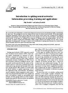
Figure 4: Top-left: input-to-hidden weights, by hidden unit. Every hidden unit has 5 incoming connections: weights 1-5 go to HU 1, weights 6-10 to HU 2, etc. Bottom-left: hidden-to-output weights. Right: the network. Dotted lines correspond to connections that are one order of magnitude lower than those in solid line. A vertical line through a cell corresponds to an active threshold.

Non-linear modeling The second step is to use a neural network to perform the idlentification. We use a 4-10-1 network to try to fit the data. This neural network model contains 61 parameters (including bias), which can be considered as slightly over-parameterized, compared to the 200 data at hand. Training is performed as a.bove, by minimizing the regularized cost (3). The regularization parameter is tuned using an additional set of 100 data, and the performance is evaluated on the 10,000 data of the validation set. Results Figure 4 displays a plot comparable to figure 1, but for our system identification case. One can see that among the 10 hidden units originaly in the model, only 1 remains in use. All the other hidden units have been pruned out of the network. The table 'below summarizes the results obtained by both the linear and the non-linear model 011 the noisy training set and on the non-noisy validation set. In this table, N N means Neural Networks. The numbers indicated are the mean squared error (MSE) over the training (resp. validation) set3. Number of parameters Unregularized N N Regularized N N

Training set (200 data) 0.095 0.150

Validation set (10,000 data) 0.120 0.122 0.053

These resu.lts show that the non-linear regularized model predictably achieves 3The performance on the validation set is higher as w e chose to validate on non-noisy data, w h e n the training set has a relatively high level of noise.

59


performance well above the linear model. Furthermore, the use of the pruning prior limits the number of parameters to roughly the same amount as for the linear model. The parameters show the same pattern as in the linear case: the main contribution arises from ~ ( tand ) y(t - 2). The influence of the other inputs and the non-linearity of the model allow for an error that is half that of the linear model.

SUMMARY This paper adressed the use of a regularization function that is different from the traditional weight-decay. It has sound motivation: it corresponds to the use of a Laplace distribution as a prior on the weight distribution, instead of' the usual Gaussian prior. This formal regularization also provides for structural regularization by pruning unnecessary weights. The use of the pruning prior is backed by encouraging experiments performed both on time series processing, with the well-known sunspots series, and on system identificat,ion. Our experience with the pruning prior is generaly positive. Its use provides the expected results in a convincing way.

ACKNOLEDGEMENT This work was performed thanks to a grant from the Danish Rector's Conference. Acknoledgements are gratefully directed to Patrick Gallinari for coments on a earlier draft of this paper. I am especialy indebted to Lars Kai Hansen for numerous comments and ideas related to this study.

REFERENCES [l] L. Bottou and Y . Le Cun. SN: A simulator for connectionist, models. In NeuroNimes 88, pages 371-382, Nimes, France, 1988. [2] J. Denker, D. Schwartz, B. Wittner, S. Solla, R. Howard, L. Jackel, and J . Hopfield. Large automatic learning, rule extraction, and generalization. Complex Systems, 1:877-922, 1987. [3] C. Goutte and L. K. Hansen. Regularization with a pruning prior. Neural Networks, submitted 1995. preprint available at ftp://ei.dtu.dk/. [4] B. Hassibi and D. G. Stork. Second order derivatives for network pruning: Optimal brain surgeon. In S.J. Hanson, J.D. Cowan, and C.L. Giles, editors, Advances in Neural Information Processing Systems, volume 5 of NIPS, pages 164-171. Morgan Kaufmann, 1993.

60


[5] A . Krogh and J. A. Hertz. A simple weight, decay can improve generalization. In J. E. Moody, S. J. Banson, and R. P. Lippman, editors, Advances in Neural Information Processing Systems, volume 4 of NIPS, 1992.

[6] Y. Le Cun, J . S. Denker, and S. A. Solla. Optimal brain damage. In D. S. Touretzky, editor, Advances in Neural Information Processing Systems, volume 2 of NIPS, pages 598-605. Morgan-Kaufmann, 1990.

[7] L. Ljung, J . Sjoberg, and T. McKelvey. On the use of regularization in system identification. Technical Report 1379, Department of Electrical Engineering, Linkoping University, S-58 1 83 Linkoping, Sweden, 1992. [SI W. H. Press, S. A . Teukolsky, W. T. Vetterling, and B. P. Flannery. Numerical Recipes in C. Cambridge University Press, 2nd edition, 1992.

[9] C. Svarer, L.K. Hansen, and J . Larsen. On design and evaluation of tapped-delay neural network architectures. In H.R. Berenji et al., editor, IEEE International Conference on Neural Networks, IC”, pages 46-51, Piscataway, N J , 1993. IEEE.

[lo] A S. VVeigend, B. A. Huberman, and D. E. Rumelhart. Predicting the future: a connectionist approach. International .Journal of Neural Systems, 1(3):193-210, 1990 [ll] P. M. Williams Bayesian regularization and pruning using a laplace prior. Neural Computation, 7(1):117-143, 1995.

[la] G . U . Yule. On a inethod of investigating periodicities in disturbed series with special reference to Wolfer’s sunspot numbers Philos. Trans. R. Soc. Lond. Ser. A , 226:267, 1927.

61
