Abstract| In this paper neural network approach for nonlinear noise and interference cancellation is de- veloped . The Hyper Radial Basis Function (HRBF).
NONLINEAR INTERFERENCE CANCELLATION USING NEURAL NETWORKS Andrzej Cichocki, Sergiy A. Vorobyov, and Tomasz Rutkowski Lab. for Open Information Systems, Riken, Brain Science Institute 2-1 Hirosawa, Saitama 351-0198 Wako-shi, Japan cia(svor,tomek)@open.brain.riken.go.jp
Abstract| In this paper neural network approach
for nonlinear noise and interference cancellation is developed . The Hyper Radial Basis Function (HRBF) neural network with associated Manhattan learning algorithm is proposed for noise cancellation under assumption that reference noise is available. Extended multichannel model with multi-references noise signal is also presented and fast learning algorithm is developed. Performance and validity of the learning algorithms are illustrated by simulation.
I. INTRODUCTION
In many applications, especially in biomedical signal processing the source signals are corrupted by various interferences and noises. Optimum noise cancellation usually requires nonlinear dynamic system for e�cient noise cancellation [3], [4], [7]. Traditional linear Finite Impulse Response (FIR) adaptive lter may not achieve acceptable level of noise cancellation for many real-world problems since noise signals are related to available (measured) reference signals in a complex dynamic and nonlinear way [1], [7]. In this paper we propose to use HRBF neural network rst proposed by Poggio and Girosi [9]. Most of the work about linear and nonlinear noise cancellation assume that additive noise can be modeled as Gaussian process [2] - [8]. In this paper we relax this assumption and we investigate several neural network models and associated adaptive learning algorithms for optimal noise cancellation.
II. PROBLEM FORMULATION
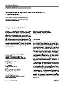
The basic problem is illustrated in Fig.1. We observe corrupted by additive noise source signal d(k )
=
s(k ) + � (k );
(1)
where s(k) is the unknown primary source signal and is the undesired interference or noise signal. We assume that only noisy signal d(k) and reference noise �R (k ) are available. Moreover, we assume that between reference noise �R (k) and noise � (k) exist unknown nonlinear dynamic relationship described by � (k )
Unknown
s(k ) +
S
d (k ) +
_S
+ n (k )
H n
R
(k)
sˆ(k ) n ˆ(k )
W
Figure 1: Interference cancelling principle with reference noise �R .
nonlinear lter H. Our objective is to design an appropriate neural network which estimates nonlinear lter H in such a way that we estimate optimally noise � (k) and subtract it from signal d(k) (see Fig.1). So, primary source signal can be estimated. In many applications we have several observation of the same signal as di (k ) = gi s(k ) + �i (k ); (i = 1; 2; :::; l); (2) where scaling coe�cients gi are unknown and �i (k) are additive noises. Our objective is to estimate original source signal s(k) taking into account all available information.
III. HYPER RADIAL BASIS FUNCTION NETWORK FOR NONLINEAR INTERFERENCE CANCELLATION
A HRBF network have been introduced rst by Poggio and Girosi [9]. The main idea is to consider the mapping to be approximated (for our problem, it is nonlinear lter W) as the sum of several radial basis functions, each one with its own prior, that is stabilizer. The corresponding regularization principle then yields a superposition of di�erent Green's functions, in particular Gaussian functions, with di�erent widths. We are interested here in the special case of Green's functions that allow us to consider HRBF network as a twolayer neural network in which the hidden layer perform an adaptive nonlinear transformation with adjustable weight parameters so that M dimensional input space � R (k ) = [�R (k ); �R (k ; 1); :::; �R (k ; M + 1)]> is
Unknown
Nonlinear Adaptive Filter (HRBFN)
n R(k)
z-
H
F
1
2
( r )1
+ +
M F
n
( r )n
S
s(k) M
+
n ˆ(k)
G s2(k)
s1(k)
+
d(k)
S
_
S
+
S
n
n n
R1
(k )
R2
(k )
Rl
n X
=
w0
+
=
w0
+ w> �(�);
j =1
wj �j (�j )
(3)
where w = [w1 ; w2 ; :::; wn ]> 2 Rn is the vector of weights, �(�) = [�1 (�1 ); �2 (�2 ); :::; �n (�n )]> is the vector consist of generalized Gaussian functions �j (�j ) = 21 exp(; 12 �2j ) and �2j = k Qj (� R(k) ;cj ) kh2 = (� R (k) ; cj )> Q>j Qj (� Ri (k) ; cj ) = 2 PM PM �& �=1 & =1 qj (�R (k ; & + 1) ; cj& ) ; j = 1; :::; n, with adaptive centers cj = [cj1 ; :::; cjM ]> and Qj are covariance matrices (see also Fig.2). Note that if (M � M ) positive de nite matrix Q>j Qj reduces to ;2 ) the HRBF neta diagonal matrix diag(�j;12 ; :::; �jM work is simpli ed to the RBF neural network. For identi cation of nonlinear lter W using HRBF network we must estimate all parameters: wi , i = 0; 1; :::; n, cj and Qj . Unfortunately, for interference cancellation problem, there is no explicit training set of input-output examples for HRBF network learning. The objective becomes minimization of the power of the output signal s^(k), which can be written as s^(k )
= =
; �^(k) ; w> �(�):
e(k ) = d(k ) d(k ) w0
;
(4)
Our objective now is to estimate all free parameters � = fw; fcj g; fQj gg of HRBF network using standard multi-step or one-step power function like following function 1 2 1 2 (5) J (�) = 2 e (k) = 2 s^ (k): To avoid stacking in local minima we apply Manhattan learning formula of the form [10]: �(k) = �(k ; 1) ; �(k) sign @J@(�) � ; (6)
M
d2(k)
d1(k)
+
V
d(k) +
S
sˆ(k) _
n 2(k) L n l (k) l
H n ˆ(k)
(k )
cancellation.
mapped to the one-dimensional output space �^(k): RM ! R as
dl (k) +
W
M
Figure 2: Model of HRBF network for nonlinear interference
�^(k )
S
H1 H2 L H
sˆ(k)
e(k) = sˆ(k) = d(k) - n ˆ(k)
Learning Alghoritm
+
n 1(k) +
+
M
M
+
wn
S
Unknown
sl (k)
w0
w2
( r )2
1
M
s(k) + +
1
z-
n (k)
F
w1
HRBF Network
Figure 3: Multichannel nonlinear interference cancellation model.
where �(k) is self-adaptive learning steps. In the simplest case �(k) may be xed. Gradient components for all free parameters are @J (�)
= ;(d(k) ; �^(k)); r = ;�(�)(d(k) ; �^(k)); = �j Qj (� R (k) ; cj )(� R (k) ; cj )> ; @ Qj rc J (�) = ;�j Q>j Qj (� R (k) ; cj ); (7) @w0 w J (�) @J (�) j
where �j = 12 wj exp(; 12 (� R(k) ; cj )> Q>j Qj (� R (k) ; cj ))(d(k) ; �^(k)) = wj �j (�j )(d(k) ; �^(k)). Note that HRBF network is extension of the RBF network and it can be proved that it will work good ever if the sequences � (k) and �R (k) have non-Gaussian distribution (for example, Laplacian or Cauchy distribution).
IV. EXTENDED MULTICHANNEL MODEL WITH MULTI-REFERENCES NOISE SIGNAL
In this section we consider more sophisticated model shown in Fig.3. In this model we assume that we observe l noisy signals di (k) (see Eq. (2)). We also observe l reference noises that are uncorrelated with a source signal s(k) but are related in nonlinear way, represented symbolically by lters Hi , to noises �i (k). We use the algorithm proposed in last section for estimation of HRBF network W weights only with one di�erence: the vector � R (k) now is � R (k) = [�R1 (k); �R1 (k ; 1); :::; �R1 (k ; M1 +1); �R2 (k); �R2 (k ; 1); :::; �R2 (k ; M2 +1); :::; �Rn (k); �Rl (k ; 1); :::; �Rl (k ; Ml + 1)]> . The original source signal is reconstructed by linear network s^(k )
=
l X i=1
vi di (k )
; �^(k) = v> d(k) ; �^(k)
(8)
with constraint
v> el = 1;
(9) because we should take into account that onedimension corrupted signal d(k) must be unbiased. Here v = [v1 ; v2 ; :::; vl ]> is (l � 1) weight vector of linear network V, d(k) = [d1 (k); d2 (k); :::; dl (k)]> and el = [1; 1; :::; 1]> is (l � 1) vectors. Minimization of cost function J
= 21
N X k=1
s^2 (k )
= 12
N X (v> d(k) ; �^(k))2 ; k=1
(10)
N X = 12 (v> d(k) ; �^(k))2 k=1 + �(v> el ; 1):
(11)
Hence, Kuhn-Tucker equations can be expressed as N X d>(k)vd(k)
rv k L = ( )
k=1 N X
; @L @�
k=1
d(k)^� (k) ; �el = 0;
v> el ; 1 = 0;
=
(12)
where � is nonnegative Lagrange multiplier, N is the width of window. Introducing into consideration new de ;1 = nitions for errors � �;1 covariance matrix P PN > and least mean square estimak=1 d(k )d (k ) �P
�;1 �P
�
N tion v~ = Nk=1 d(k)d> (k) � (k ) the k=1 d(k )^ solution of the system (12) can be given by: e>v~ ; 1 ; � = 2 l
e>l P; el > v~ ; P; ee>l Pv~;; e1 el : 1
v
=
(13)
1
1
l
l
Finally using Sherman-Morrison lemma about recursive matrix inversion we obtain following learning algorithm for on-line tuning of vector v(k) of linear network V:
P; (k) 1
v~ (k)
P;; (k ; 1) > ; ; P 1(k+;d>1)(dk()kP);d ((kk;)P1)d((kk); 1) ; = v~ (k ; 1) ; 1)d(k)^s(k) + 1 +Pd> ((kk); P; (k>; 1)d(k) ; = v~ (k) ; P; (k) e>l v~;(k) ; 1 el : (14) el P (k)el =
1
1
1
1
1
1
v(k)
V. SIMULATION AND COMPARISON RESULTS
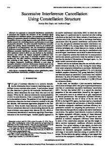
In this section, we shortly present some simulation results for the adaptive nonlinear interference canceler using HRBF network and comparison results for standard RBF �network �^(k) = w0 + � PM � R (k);c k2 k , (here �i are width pai=1 wi exp ; �2 rameters) with Stochastic Gradient (SG) learning algorithm [3] and HRBF network, proposed in this paper. Performances of the nonlinear interference canceller based on HRBF and RBF networks were measured by the normalized mean square error i
i
under constraints (9) lead to the Lagrangian L
It is obvious that we can achieve more precise estimate of s^(k) and better convergence using multireferences noise signal network than scalar reference noise signal network.
1
1
s(k )) g = E f(^sE(kf)� ; 2 (k )g PK (^s(k) ; d(k))2 ; = k=1 PK 2 k=1 � (k )
N M SE
2
(15)
where K is the number of iterations during learning period. The initial weights wj , (j = 0; 1; 2; :::; n) of the HRBF and RBF networks were all initialized to small random values. The initial values of centers for RBF network were determined by K -means clustering on the rst 100 samples of the input data and initial width parameters �i were set to the average of the M nearestneighbor distances among the initialized centers. For HRBF network initial values of centers and components of matrices Qj , j = 1; 2; :::; M were chosen to small random values. If we would choose initial condition for HRBF network as follow: for centers as K -mean clusters that had obtained using 100 samples of the input data and for Qj : qiij = �j , qikj = 0 for all i 6= k, then RBF and HRBF would be quite equivalent before learning. So RBF network had a little bit more \convenient" initial conditions in our simulation than HRBF network. Due to limit of space we present here only one illustrative example. The signal s(k) and the reference noise were given by s(k) = 0:7 cos(2�0:1k) + 0:3 sin(2�0:25k); �R (k) = sin(2�0:06k + �(k)), where �(k ) is the random phase generated according Laplace pdf with �� = 0:003. Interference noise signal was � (k) = cos(2�0:06k) ; 0:5 sin2 (2�0:06(k ; 1)) + (cos(2�0:06k) ; 0:5 sin2 (2�0:06(k ; 1)))2 : The interference canceller has to estimate the deterministic interference � (k) using samples of the reference input �R (k) with a random non-Gaussian phase noise. The relationship between �R (k) and � (k) is highly nonlinear and also the phase of reference signal
3
Real interference
2
2 1 0
0 −1
−1 −2
1
0
50
100
0
50
100
150
200
250
0
50
100
150
200
250
0
50
100
150
200
250
3
150
using RBFN
Time
60 50 40
2 1 0 −1
30 20
2
0 −10
0
50
100
150
200
250 Frequency
300
350
400
450
500
Figure 4: Waveforms and magnitude spectra for signals d(k) -, s(k) - . - and � (k) * . −5
NMSE in dB
−10
−15
−20
−25
−30
0
1000
2000
3000
4000
5000 Time
6000
7000
8000
9000
10000
Figure 5: Normalized mean square error for RBF - and HRBF * networks.
randomly uctuate. Fig. 4 shows the time waveforms and spectra of the corrupted signal d(k) = s(k)+ � (k), the useful and interference signals s(k) and � (k). Due to size limitation we show the simulation results for only one con guration of networks, with M = 5 delays and n = 20 hidden units both for RBF and HRBF networks. Figs.5, 6, 7 show respectively: Fig.5 - normalized mean square error for RBF and HRBF networks; Fig.6 - the output spectra of RBF and HRBF networks spectra for K = 10000; and Fig.7 - the original reference signal � (k) and its estimation �^(k) using RBF and HRBF networks on the last 200 learning iterations. We can see that HRBF network is able to learn more rapidly and allow to achieve smaller value of normalized mean square error than the standard RBF network. These results are similar for other con guration of RBF and HRBF networks and are general. Hence, these results suggest that the nonlinear canceller based on the HRBF network performed much better than the canceller based on the standard RBF network. However, it should be noted that HRBF network is sensitive to initial values of self-adaptive learning steps for learning algorithm. Hence, generally speaking, the procedure for adjustment of learning steps can be added to the algorithm.
0 −1
Figure 7: Original reference signal � (k) and its estimations using RBF and HRBF networks.
References
[1] A. Cichocki, W. Kasprzak, S. Amari, \Adaptive approach to blind source cancellation of additive and convolutional noise", ICSP'96, Int. Conf. on Signal Processing, Beijing, China, pp.412-415, 1996. [2] B. Widrow, S.D. Stearn, \Adaptive Signal Processing", Prentice-Hall, S.P.Series, 1985. [3] I. Cha and S.A. Kassam, \Interference cancellation using radial basis function networks", Signal Processing, vol.47, pp.247-268, 1995. [4] I. Cha and S.A. Kassam, "Channel equalization using adaptive complex radial basis function networks", IEEE Journal on Selected Areas in Communications, vol.13, No.1, pp.122-131, 1995. [5] Y. Lu, N. Sundararajan and P. Saratchandran, "Performance evaluation of a sequential minimal radial basis function (RBF) neural network learning algorithm", IEEE Trans. Neural Networks, vol.9, No.2, pp.308-318, 1998. [6] E. Bataillou and H. Rix, "A new method for noise cancellation", Proc. of Conf. on Signal Processing VII: Theories and Applications, pp.1046-1049, 1994. [7] W.G. Knecht, M.E. Schenkel and G.S. Moschytz "Nonlinear lters for noise reduction", Proc. of Conf. on Signal Processing VII: Theories and Applications, pp.1500-1503, 1994. [8] C. Serviere, D. Baudois, A. Silvent, "Noise cancelling with signal and reference correlated, using third order moments", (in book Higher Order Statistics), 1992, pp.279-282. [9] T. Poggio and F. Girosi, "Network for approximation and learning", Proc. of the IEEE, vol.78, pp.14811497, 1990. [10] A. Cichocki, and R. Unbehauen, \Neural Networks for Optimization and Signal Processing", J. Wiley, 1994.
60
50
40
30
20
10
0
1
�^(k)
0
−35
using HRBFN
10
0
50
100
150
200
250 Frequency
300
350
400
450
500
Figure 6: Output spectra of RBF - and HRBF * networks.