Nonlinear spectral unmixing of hyperspectral images

THÈSE En vue de l’obtention du

DOCTORAT DE L’UNIVERSITÉ DE TOULOUSE Délivré par : l’Institut National Polytechnique de Toulouse (INP Toulouse)

Présentée et soutenue le 07/10/2013 par :

Yoann ALTMANN

Nonlinear spectral unmixing of hyperspectral images Démélange non-linéaire d’images hyperspectrales

Olivier CAPPÉ Jocelyn CHANUSSOT Jérome IDIER Cédric RICHARD Steve MCLAUGHLIN Véronique SERFATY Jacques BLANC-TALON Manuel GRIZONNET Jean-Yves TOURNERET Nicolas DOBIGEON

JURY Directeur de recherche CNRS Professeur à l’INPG/GIPSA-Lab Directeur de recherche CNRS Professeur à l’Université Nice Sophia-Antipolis Professeur à l’Université Heriot-Watt Responsable Domaine Scientifique DGA Responsable Domaine Scientifique DGA Ingénieur CNES Professeur à l’INPT-ENSEEIHT Maître de conférence à l’INPT-ENSEEIHT

École doctorale et spécialité : MITT : Image, Information, Hypermedia Unité de Recherche : Institut de Recherche en Informatique de Toulouse (UMR 5505) Directeur(s) de Thèse : Jean-Yves TOURNERET et Nicolas DOBIGEON Rapporteurs : Jocelyn CHANUSSOT , Jérome IDIER et Cédric RICHARD

Président Rapporteur Rapporteur Rapporteur Examinateur Examinatrice Invité Invité Directeur de these Co-directeur de these

Remerciements Je remercie tout d'abord mon directeur de thèse Jean-Yves Tourneret et mon co-directeur de thèse Nicolas Dobigeon sans qui le travail réalisé durant ces trois ans n'aurait pas pu aboutir. Je les remercie pour leur grande disponibilité, leurs larges compétences, leurs idées et leurs commentaires qui m'ont tiré vers le haut. Je les remercie également de m'avoir donné l'opportunité de rencontrer les nombreuses personnes avec qui j'ai eu l'occasion de discuter durant cette thèse. Je tiens à exprimer mes remerciements les plus sincères aux membres du jury de thèse qui ont accepté de juger ce travail. Je suis profondément reconnaissant à mes trois rapporteurs, M. Jocelyn Chanussot, M. Jérôme Idier et M. Cédric Richard, d'avoir accepté de lire et évaluer ma thèse. Je remercie également M. Olivier Cappé, M. Steve McLaughlin, et Mme Véronique Serfaty, qui ont accepté d'être examinateurs de ma thèse. Cette thèse n'aurait pas pu se faire sans le support de la Direction Générale de l'Armement (DGA), et en particulier Mme Véronique Serfaty qui m'a suivi pendant ces trois années. Je remercie tous mes collègues de l'IRIT, enseignants, chercheurs, doctorants, techniciens, secrétaires, pour leur sympathie et convivialité au sein du laboratoire. Merci pour les aides permanentes reçues du personnel du laboratoire. Je n'oublie pas mes visites à Edimbourg durant lesquelles j'ai eu l'occasion de rencontrer et de discuter avec de nombreuses personnes et je remercie M. Steve McLaughlin pour son accueil, sa convivialité et sa disponibilité. Je suis persuadé que le post-doc à Heriot-Watt sera une expérience exceptionnelle. Je remercie particulièrement Abderrahim, Cécile, Julien Renaud, Bouchra, Soksok, Olivier, Romain, de l'IRIT, sans oublier Raoul, Victor, Florian, Chao, Jorge et Jean-Adrien du Tésa pour ces trois années. Une pensée à ma famille et mes amis qui m'ont encouragé durant ma thèse. Je remercie mes parents de m'avoir permis de poursuivre mes études et je leur exprime toute mon aection et ma gratitude. Enn, et j'aurais tout aussi bien pu commencer ces remerciements par elle, je remercie

amore mio,

celle qui

m'accompagne, me soutient et qui a largement contribué à cette thèse. Je lui doit beaucoup et plus encore. Merci à tous.

iii

Résumé Le démélange spectral est un des sujets majeurs de l'analyse d'images hyperspectrales.

Ce problème consiste à

identier les composants macroscopiques présents dans une image hyperspectrale et à quantier les proportions (ou abondances) de ces matériaux dans tous les pixels de l'image. La plupart des algorithmes de démélange suppose un modèle de mélange linéaire qui est souvent considéré comme une approximation au premier ordre du mélange réel. Cependant, le modèle linéaire peut ne pas être adapté pour certaines images associées par exemple à des scènes engendrant des trajets multiples (forêts, zones urbaines) et des modèles non-linéaires plus complexes doivent alors être utilisés pour analyser de telles images. Le but de cette thèse est d'étudier de nouveaux modèles de mélange non-linéaires et de proposer des algorithmes associés pour l'analyse d'images hyperspectrales.

Dans un premier temps, un modèle paramétrique post-non-

linéaire est étudié et des algorithmes d'estimation basés sur ce modèle sont proposés. Les connaissances a priori disponibles sur les signatures spectrales des composants purs, sur les abondances et les paramètres de la nonlinéarité sont exploitées à l'aide d'une approche bayesienne.

Le second modèle étudié dans cette thèse est basé

sur l'approximation de la variété non-linéaire contenant les données observées à l'aide de processus gaussiens. L'algorithme de démélange associé permet d'estimer la relation non-linéaire entre les abondances des matériaux et les pixels observés sans introduire explicitement les signatures spectrales des composants dans le modèle de mélange. Ces signatures spectrales sont estimées dans un second temps par prédiction à base de processus gaussiens. La prise en compte d'eets non-linéaires dans les images hyperspectrales nécessite souvent des stratégies de démélange plus complexes que celles basées sur un modèle linéaire. Comme le modèle linéaire est souvent susant pour approcher la plupart des mélanges réels, il est intéressant de pouvoir détecter les pixels ou les régions de l'image où ce modèle linéaire est approprié. On pourra alors, après cette détection, appliquer les algorithmes de démélange nonlinéaires aux pixels nécessitant réellement l'utilisation de modèles de mélange non-linéaires. La dernière partie de ce manuscrit se concentre sur l'étude de détecteurs de non-linéarités basés sur des modèles linéaires et non-linéaires pour l'analyse d'images hyperspectrales. Les méthodes de démélange non-linéaires proposées permettent d'améliorer la caractérisation des images hyperspectrales par rapport au méthodes basées sur un modèle linéaire. Cette amélioration se traduit en particulier par une meilleure erreur de reconstruction des données. De plus, ces méthodes permettent de meilleures estimations des signatures spectrales et des abondances quand les pixels résultent de mélanges non-linéaires. Les résultats de simulations eectuées sur des données synthétiques et réelles montrent l'intérêt d'utiliser des méthodes de détection de non-linéarités pour l'analyse d'images hyperspectrales. En particulier, ces détecteurs peuvent permettre d'identier des composants très peu représentés et de localiser des régions où les eets non-linéaires sont non-négligeables (ombres, reliefs,...). Enn, la considération de corrélations spatiales dans les images hyperspectrales peut améliorer les performances des algorithmes de démélange non-linéaires et des détecteurs de non-linéarités.

v

Abstract Spectral unmixing is one the major issues arising when analyzing hyperspectral images. It consists of identifying the macroscopic materials present in a hyperspectral image and quantifying the proportions of these materials in the image pixels.

Most unmixing techniques rely on a linear mixing model which is often considered as a rst

approximation of the actual mixtures. However, the linear model can be inaccurate for some specic images (for instance images of scenes involving multiple reections) and more complex nonlinear models must then be considered to analyze such images. The aim of this thesis is to study new nonlinear mixing models and to propose associated algorithms to analyze hyperspectral images. First, a post-nonlinear model is investigated and ecient unmixing algorithms based on this model are proposed. The prior knowledge about the components present in the observed image, their proportions and the nonlinearity parameters is considered using Bayesian inference. The second model considered in this work is based on the approximation of the nonlinear manifold which contains the observed pixels using Gaussian processes. The proposed algorithm estimates the relation between the observations and the unknown material proportions without explicit dependency on the material spectral signatures, which are estimated subsequentially. Considering nonlinear eects in hyperspectral images usually requires more complex unmixing strategies than those assuming linear mixtures. Since the linear mixing model is often sucient to approximate accurately most actual mixtures, it is interesting to detect pixels or regions where the linear model is accurate. This nonlinearity detection can be applied as a pre-processing step and nonlinear unmixing strategies can then be applied only to pixels requiring the use of nonlinear models. The last part of this thesis focuses on new nonlinearity detectors based on linear and nonlinear models to identify pixels or regions where nonlinear eects occur in hyperspectral images. The proposed nonlinear unmixing algorithms improve the characterization of hyperspectral images compared to methods based on a linear model. These methods allow the reconstruction errors to be reduced. Moreover, these methods provide better spectral signature and abundance estimates when the observed pixels result from nonlinear mixtures. The simulation results conducted on synthetic and real images illustrate the advantage of using nonlinearity detectors for hyperspectral image analysis. In particular, the proposed detectors can identify components which are present in few pixels (and hardly distinguishable) and locate areas where signicant nonlinear eects occur (shadow, relief, ...). Moreover, it is shown that considering spatial correlation in hyperspectral images can improve the performance of nonlinear unmixing and nonlinearity detection algorithms.

vii

Acronyms and notations Acronymes ARE

average reconstruction error

CCRLB

constrained Cramér-Rao lower bound

CHMC

constrained Hamiltonian Monte Carlo

CRLB

Cramér-Rao lower bound

CHMC

constrained Hamiltonian Monte Carlo

DAG

directed acyclic graph

EEA

endmember extraction algorithm

FCLL-GPLVM

fully constrained locally linear Gaussian process latent variable model

FM

Fan bilinear model

GBM

generalized bilinear model

GLRT

generalized likelihood ratio test

GP

Gaussian process

GPLVM

Gaussian process latent variable model

HMC

Hamiltonian Monte Carlo

i.i.d.

independent and identically distributed

K-FCLS

kernel fully constrained least squares

LL-GPLVM

locally linear Gaussian process latent variable model

LMM

linear mixing model

LS

least-squares

MAP

maximum a posteriori

MCMC

Markov chain Monte Carlo

MMSE

minimum mean square error

MLE

maximum likelihood estimator

MRF

Markov random eld

MSE

mean square error

NLMM

nonlinear mixing model

PCA

principal component analysis

PPNMM

post nonlinear mixing model

RCA-SU

residual component analysis-based spectral unmixing

RNMSE

root normalized mean square error

ix

RKHS

reproducing kernel Hilbert space

SAM

spectral angle mapper

SNR

signal-to-noise ratio

SO

subgradient optimization

SU

spectral unmixing

Standard notations ∝

proportional to

∼

distributed according to

much lower

much greater

Γ(·)

Gamma function

B(·, ·)

Beta function

δ(·)

Dirac delta function

Hadamard product

⊗

Kronecker product

1E (x)

indicator function dened on

  E 

1E (x) = 1 1E (x) = 0

if

x∈E

else.

Matrix notations x

scalar value

x

column vector

·T

transpose operator

X xn xn,: tr(X) etr(X) |X|

matrix

nth

column of the matrix

X

column vector consisting of the trace of the matrix

nth

row of the matrix

X

exponential trace of the matrix determinant of the matrix

1d

d×1

ones vector

0d

d×1

zeros vector

Id

d×d

identity matrix

kxk

standard

`2 -norm kxk =

X

X

√

xT x

x

X

Spectral unmixing notations R

number of endmembers

r

endmember index

N

number of pixels

n

pixel index

L

number of spectral bands

`

band index

y

pixel spectrum

a

abundance vector

mr

rth

M

endmember matrix

endmember spectrum

Sampling notations NMC

length of the Markov chain

Nbi

length of the burn-in period of the Markov chain

NLF

number of leap-frog steps

x

(k)

k -th

sample of the chain

x(k)

k=1,...,NMC

Usual distributions UE (x) N m, σ

uniform distribution dened on the set

2

NE (m, σ 2 )

Gaussian distribution with mean

m

E

and variance

σ2

truncated Gaussian distribution, whose support is and with hidden mean

m

and hidden variance

σ

E

2

N (m, Σ)

multivariate Gaussian distribution with mean

NE (m, Σ)

truncated multivariate Gaussian distribution, whose support is and with hidden mean

m

m

and covariance matrix

and hidden covariance matrix

IG(γ, ν)

inverse-gamma distribution with shape parameter

Be(α, β)

Beta distribution with shape parameters

α

and

xi

β.

γ

Σ

E

Σ

and scale parameter

ν.

xii

Contents Remerciements

iii

Résumé

v

Abstract

vii

Acronyms and notations

ix

Introduction (in French)

1

Introduction

5

1 Polynomial post-nonlinear mixing model for spectral unmixing

17

1.1

Introduction (in French) . . . . . . . . . . . . . . . . . . . . . . . . . . . . . . . . . . . . . . . . . . .

17

1.2

Introduction . . . . . . . . . . . . . . . . . . . . . . . . . . . . . . . . . . . . . . . . . . . . . . . . . .

19

1.3

Polynomial Post-Nonlinear Mixing Model

. . . . . . . . . . . . . . . . . . . . . . . . . . . . . . . . .

19

1.4

Supervised PPNMM-based unmixing . . . . . . . . . . . . . . . . . . . . . . . . . . . . . . . . . . . .

20

1.4.1

Bayesian estimation

. . . . . . . . . . . . . . . . . . . . . . . . . . . . . . . . . . . . . . . . .

21

1.4.2

Least squares methods . . . . . . . . . . . . . . . . . . . . . . . . . . . . . . . . . . . . . . . .

25

1.4.3

Simulations . . . . . . . . . . . . . . . . . . . . . . . . . . . . . . . . . . . . . . . . . . . . . .

28

1.4.4

Intermediate conclusion

36

1.5

. . . . . . . . . . . . . . . . . . . . . . . . . . . . . . . . . . . . . . .

Unsupervised PPNMM-based unmixing

. . . . . . . . . . . . . . . . . . . . . . . . . . . . . . . . . .

37

1.5.1

Bayesian estimation

. . . . . . . . . . . . . . . . . . . . . . . . . . . . . . . . . . . . . . . . .

37

1.5.2

Simulations . . . . . . . . . . . . . . . . . . . . . . . . . . . . . . . . . . . . . . . . . . . . . .

45

1.5.3


. . . . . . . . . . . . . . . . . . . . . . . . . . . . . . . . . . . . . . .

55

1.6

Conclusion

. . . . . . . . . . . . . . . . . . . . . . . . . . . . . . . . . . . . . . . . . . . . . . . . . .

56

1.7

Conclusion (in French) . . . . . . . . . . . . . . . . . . . . . . . . . . . . . . . . . . . . . . . . . . . .

57

2 Unsupervised nonlinear unmixing using Gaussian processes

59

2.1


59

2.2

Introduction . . . . . . . . . . . . . . . . . . . . . . . . . . . . . . . . . . . . . . . . . . . . . . . . . .

61

2.3

Nonlinear mixing model

. . . . . . . . . . . . . . . . . . . . . . . . . . . . . . . . . . . . . . . . . . .

63

2.4

Bayesian model . . . . . . . . . . . . . . . . . . . . . . . . . . . . . . . . . . . . . . . . . . . . . . . .

65

2.4.1

Marginalizing

W

. . . . . . . . . . . . . . . . . . . . . . . . . . . . . . . . . . . . . . . . . . .

xiii

67

2.4.2

Subspace identication . . . . . . . . . . . . . . . . . . . . . . . . . . . . . . . . . . . . . . . .

67

2.4.3

Parameter priors . . . . . . . . . . . . . . . . . . . . . . . . . . . . . . . . . . . . . . . . . . .

68

2.4.4

Marginalized posterior distribution . . . . . . . . . . . . . . . . . . . . . . . . . . . . . . . . .

69

2.4.5

Estimation of

P

. . . . . . . . . . . . . . . . . . . . . . . . . . . . . . . . . . . . . . . . . . .

70

2.5

Scaling procedure . . . . . . . . . . . . . . . . . . . . . . . . . . . . . . . . . . . . . . . . . . . . . . .

71

2.6

Gaussian process regression

. . . . . . . . . . . . . . . . . . . . . . . . . . . . . . . . . . . . . . . . .

72

2.7

Simulations on synthetic data . . . . . . . . . . . . . . . . . . . . . . . . . . . . . . . . . . . . . . . .

74

2.7.1

Subspace identication . . . . . . . . . . . . . . . . . . . . . . . . . . . . . . . . . . . . . . . .

74

2.7.2

Abundance and endmember estimation

. . . . . . . . . . . . . . . . . . . . . . . . . . . . . .

75

2.7.3

Performance in absence of pure pixels

. . . . . . . . . . . . . . . . . . . . . . . . . . . . . . .

76

2.7.4

Performance with respect to endmember variability . . . . . . . . . . . . . . . . . . . . . . . .

77

2.8

Application to a real dataset

. . . . . . . . . . . . . . . . . . . . . . . . . . . . . . . . . . . . . . . .

79

2.9

Conclusion

. . . . . . . . . . . . . . . . . . . . . . . . . . . . . . . . . . . . . . . . . . . . . . . . . .

84

2.10 Conclusion (in French) . . . . . . . . . . . . . . . . . . . . . . . . . . . . . . . . . . . . . . . . . . . .

87

3 Nonlinearity detection in hyperspectral images

89

3.1


89

3.2

Introduction . . . . . . . . . . . . . . . . . . . . . . . . . . . . . . . . . . . . . . . . . . . . . . . . . .

91

3.3

Supervised PPNMM-based nonlinearity detection . . . . . . . . . . . . . . . . . . . . . . . . . . . . .

91

3.3.1

PPNMM model and parameter estimation . . . . . . . . . . . . . . . . . . . . . . . . . . . . .

91

3.3.2

Nonlinearity detection . . . . . . . . . . . . . . . . . . . . . . . . . . . . . . . . . . . . . . . .

92

3.3.3

Constrained Cramér-Rao bound

. . . . . . . . . . . . . . . . . . . . . . . . . . . . . . . . . .

94

3.3.4

Synthetic data

. . . . . . . . . . . . . . . . . . . . . . . . . . . . . . . . . . . . . . . . . . . .

95

3.3.5

Analysis of real data . . . . . . . . . . . . . . . . . . . . . . . . . . . . . . . . . . . . . . . . . 101

3.3.6


3.4

. . . . . . . . . . . . . . . . . . . . . . . . . . . . . . . . . . . . . . . 104

Supervised LMM-based nonlinearity detection . . . . . . . . . . . . . . . . . . . . . . . . . . . . . . . 105 3.4.1

Mixing models

. . . . . . . . . . . . . . . . . . . . . . . . . . . . . . . . . . . . . . . . . . . . 105

3.4.2

Distributions of

δ 2 (y)

3.4.3

Nonlinearity detection . . . . . . . . . . . . . . . . . . . . . . . . . . . . . . . . . . . . . . . . 106

3.4.4

Simulations . . . . . . . . . . . . . . . . . . . . . . . . . . . . . . . . . . . . . . . . . . . . . . 108

3.4.5


under hypotheses

H0

and

H1

. . . . . . . . . . . . . . . . . . . . . . . 106

. . . . . . . . . . . . . . . . . . . . . . . . . . . . . . . . . . . . . . . 111

3.5

Conclusion

. . . . . . . . . . . . . . . . . . . . . . . . . . . . . . . . . . . . . . . . . . . . . . . . . . 112

3.6

Conclusion (in French) . . . . . . . . . . . . . . . . . . . . . . . . . . . . . . . . . . . . . . . . . . . . 114

4 Joint supervised unmixing and nonlinearity detection using residual component analysis

117

4.1

Introduction (in French) . . . . . . . . . . . . . . . . . . . . . . . . . . . . . . . . . . . . . . . . . . . 118

4.2

Introduction . . . . . . . . . . . . . . . . . . . . . . . . . . . . . . . . . . . . . . . . . . . . . . . . . . 119

4.3

Problem formulation . . . . . . . . . . . . . . . . . . . . . . . . . . . . . . . . . . . . . . . . . . . . . 119

4.4

Bayesian model . . . . . . . . . . . . . . . . . . . . . . . . . . . . . . . . . . . . . . . . . . . . . . . . 120 4.4.1

Likelihood . . . . . . . . . . . . . . . . . . . . . . . . . . . . . . . . . . . . . . . . . . . . . . . 120

4.4.2

Prior for the abundance matrix

A

. . . . . . . . . . . . . . . . . . . . . . . . . . . . . . . . . 121

xiv

4.4.3 4.5

4.6

Modeling the nonlinearities

4.8

4.9

. . . . . . . . . . . . . . . . . . . . . . . . . . . . . . . . . . . . . . . . . 121

Φ

4.5.1

Prior distribution for the nonlinearity matrix

4.5.2

Prior distribution for the label vector

4.5.3

Hyperparameter priors . . . . . . . . . . . . . . . . . . . . . . . . . . . . . . . . . . . . . . . . 123

z

. . . . . . . . . . . . . . . . . . . . . . . . . . 122

. . . . . . . . . . . . . . . . . . . . . . . . . . . . . . 123

Bayesian inference using a Metropolis-within-Gibbs sampler . . . . . . . . . . . . . . . . . . . . . . . 124 4.6.1

Marginalized joint posterior distribution . . . . . . . . . . . . . . . . . . . . . . . . . . . . . . 124

4.6.2

Sampling the labels

4.6.3

Sampling the abundance matrix

4.6.4

Sampling the noise variance

4.6.5 4.7

Prior for the noise variances . . . . . . . . . . . . . . . . . . . . . . . . . . . . . . . . . . . . . 121

Sampling the vector

. . . . . . . . . . . . . . . . . . . . . . . . . . . . . . . . . . . . . . . . . 125

s

2

σ2

A

. . . . . . . . . . . . . . . . . . . . . . . . . . . . . . . . . 125

. . . . . . . . . . . . . . . . . . . . . . . . . . . . . . . . . . . 126

. . . . . . . . . . . . . . . . . . . . . . . . . . . . . . . . . . . . . . . . 126

Simulations for synthetic data . . . . . . . . . . . . . . . . . . . . . . . . . . . . . . . . . . . . . . . . 127 4.7.1

First scenario: RCA vs. linear unmixing . . . . . . . . . . . . . . . . . . . . . . . . . . . . . . 127

4.7.2

Second scenario: RCA vs. nonlinear unmixing

. . . . . . . . . . . . . . . . . . . . . . . . . . 129

Simulations for a real hyperspectral image . . . . . . . . . . . . . . . . . . . . . . . . . . . . . . . . . 132 4.8.1

Data set . . . . . . . . . . . . . . . . . . . . . . . . . . . . . . . . . . . . . . . . . . . . . . . . 132

4.8.2

Spectral unmixing

4.8.3

Nonlinearity detection . . . . . . . . . . . . . . . . . . . . . . . . . . . . . . . . . . . . . . . . 133

Conclusion

. . . . . . . . . . . . . . . . . . . . . . . . . . . . . . . . . . . . . . . . . . 132

. . . . . . . . . . . . . . . . . . . . . . . . . . . . . . . . . . . . . . . . . . . . . . . . . . 135

4.10 Conclusion (in French) . . . . . . . . . . . . . . . . . . . . . . . . . . . . . . . . . . . . . . . . . . . . 137

Conclusion and future work 4.11 Conclusion

139

. . . . . . . . . . . . . . . . . . . . . . . . . . . . . . . . . . . . . . . . . . . . . . . . . . 139

4.12 Future work . . . . . . . . . . . . . . . . . . . . . . . . . . . . . . . . . . . . . . . . . . . . . . . . . . 140

Conclusion et perspectives (in French) 4.13 Conclusion

143

. . . . . . . . . . . . . . . . . . . . . . . . . . . . . . . . . . . . . . . . . . . . . . . . . . 143

4.14 Perspectives . . . . . . . . . . . . . . . . . . . . . . . . . . . . . . . . . . . . . . . . . . . . . . . . . . 144

Appendices

149

A Identiability of the supervised PPNMM-based SU problem

149

A.1

Non-injectivity of

A.2

Injectivity of

s 7→ g(s)

. . . . . . . . . . . . . . . . . . . . . . . . . . . . . . . . . . . . . . . . . 149

(a, b) 7→ g(a, b) = Ma + b(Ma) (Ma)

. . . . . . . . . . . . . . . . . . . . . . . . . . 149

B Partial derivatives for the LS PPNMM-based algorithms B.1 B.2

Partial derivatives of

ˇb(·)


ˇ∗

and

y (·)

h(·)

151

. . . . . . . . . . . . . . . . . . . . . . . . . . . . . . . . . . . . . 151

. . . . . . . . . . . . . . . . . . . . . . . . . . . . . . . . . . . . . . . . . . 151

C Derivation of the potential functions associated the UPPNMM algorithm zn

153

C.1

Derivation of the potential function associated with

C.2

Derivation of the potential functions associated with the endmember matrix . . . . . . . . . . . . . . 154

xv

. . . . . . . . . . . . . . . . . . . . . . . . . . 153

D On the linear mapping between latent variables and abundances D.1

Dimension of the subspace spanned by

D.2

Existence and rank of

D.3

Relation between

D.4

Scenario where rank(W0 )

a

W

and

x

y

155

. . . . . . . . . . . . . . . . . . . . . . . . . . . . . . . . . . 156

. . . . . . . . . . . . . . . . . . . . . . . . . . . . . . . . . . . . . . . . . . 157 . . . . . . . . . . . . . . . . . . . . . . . . . . . . . . . . . . . . . . . . . . 157

0 PR−1 cr − i=1,i6=r ci ,

27

if

dr < 0

λr,M ∈ R+ λr

(for

according to

Chapter 1. Polynomial post-nonlinear mixing model for spectral unmixing

ensures the constraints (1.4) are satised. (Bazaraa et al., 1993, p.

270).

The problem (1.35) can be solved using the golden section method

The abundances are then updated component by component.

Here again, the

procedure is repeated until convergence. The nal algorithm is summarized in Algo. 1.3. The next section presents the performance of the proposed algorithms on synthetic and real hyperspectral images.

1.4.3 Simulations

Synthetic data

The performance of the proposed nonlinear SU algorithms is rst evaluated by unmixing 4 synthetic images of size

50 × 50

pixels. The

R=3

endmembers contained in these images have been extracted from the spectral libraries

provided with the ENVI software (RSI (Research Systems Inc.), 2003) (i.e., green grass, olive green paint and galvanized steel metal). The rst synthetic image (LMM). A second image

I2

I1

has been generated using the standard linear mixing model

has been generated according to the bilinear mixing model introduced by Fan et al.

(2009), referred to as Fan model (FM). A third image

I3

has been generated according to the generalized bilinear

mixing model (GBM) presented by Halimi et al. (2011a), whereas a fourth image the PPNMM. For each image, the abundance vectors

an , p = 1, . . . , 2500

I4

has been generated according to

have been randomly generated according

to a uniform distribution over the admissible set dened by the positivity and sum-to-one constraints. All images have been corrupted by an additive white Gaussian noise of variance to-noise ratio

−1 −2

SNR = L

σ

2

kg (a)k ' 15dB.

for the GBM and the parameter

b

σ 2 = 2.8 × 10−3 ,

corresponding to a signal-

The nonlinearity coecients are uniformly drawn in the set

has been generated uniformly in the set

(−0.3, 0.3)

(0, 1)

for the PPNMM. Dierent

estimation procedures have been considered for the four mixing models. More precisely,

•

for the LMM, we have considered the standard FCLS algorithm (Heinz and C.-I Chang, 2001) and the Bayesian algorithm by Dobigeon et al. (2008),

•

the FM has been unmixed using the LS method introduced by Fan et al. (2009) and a Bayesian algorithm similar to the one derived by Halimi et al. (2011a) but assuming all the nonlinearity coecients are equal to 1,

•

the unmixing strategies used for the GBM are the three algorithms presented in (Halimi et al., 2011b), i.e., a Bayesian algorithm and two LS methods,

•

the Bayesian and LS algorithms presented in this chapter have been used for unmixing the proposed PPNMM. Note that all results presented in this study have been obtained using the Bayesian MMSE estimator.

The quality of the unmixing procedures can be measured by comparing the estimated and actual abundance vector using the root normalized mean square error (RNMSE) dened by

v u N u 1 X 2 t RNMSE = kˆ an − an k N R n=1 where

an

is the

the images

nth

I1 , . . . , I4

actual abundance vector and

ˆn a

(1.36)

its estimate. Table 1.1 shows the RNMSEs associated with

for the dierent estimation procedures. Note that the best results (in term of RNMSE) for

each image have been represented in bold and blue whereas the second best results have been depicted in bold.

28


Table 1.1: Abundance RNMSEs (×10−2 ): synthetic images .

LMM FM

GBM

I1

I2

I3

I4

(LMM)

(FM)

(GBM)

(PPNMM)

Bayesian (Dobigeon et al., 2008)

0.91

15.90

8.75

10.90

FCLS (Heinz and C.-I Chang, 2001)

0.91

14.27

5.48

9.73

Bayesian (Halimi et al., 2011b)

13.09

0.87

7.87

9.72

Taylor (Fan et al., 2009)

13.09

0.86

7.28

15.20


1.87

10.10

5.25

9.34

Taylor (Halimi et al., 2011b)

3.65

8.47

4.08

9.01

Gradient (Halimi et al., 2011b)

2.47

2.45

1.73

8.69

Bayesian

1.58

1.98

1.86

1.69

Taylor

1.56

2.21

1.88

1.92

Gradient

1.69

1.98

1.98

1.69

PPNMM

Table 1.1 shows that the abundances estimated by the Bayesian algorithm and the LS methods are similar for the PPNMM. Moreover, for these 4 images, the PPNMM seems to be more robust than the other mixing models to deviations from the actual model. The unmixing quality can also be evaluated by the average reconstruction error (ARE) dened by

v u N u 1 X 2 t kˆ yn − yn k ARE = LN n=1 where

yn

is the

nth

synthetic images.

observed pixel and

ˆn y

(1.37)

its estimate. Table 1.2 compares the AREs obtained for the dierent

These results show that the AREs are close for the dierent unmixing algorithms even if the

estimated abundances can vary more signicantly. Again, the proposed PPNMM seems to be more robust than the other mixing models to deviations from the actual model in term of ARE.

29


Table 1.2: AREs (×10−2 ): synthetic images .

LMM FM

GBM

PPNMM

I1

I2

I3

I4

(LMM)

(FM)

(GBM)

(PPNMM)


5.28

6.54

5.65

5.89


5.28

5.74

5.42

5.48

Bayesian

5.61

5.29

5.38

5.76


5.61

5.28

5.38

5.75


5.29

5.49

5.33

5.44


5.31

5.40

5.30

5.42


5.29

5.30

5.28

5.41

Bayesian

5.28

5.29

5.28

5.28

Taylor

5.29

5.29

5.28

5.28

Gradient

5.29

5.29

5.28

5.28

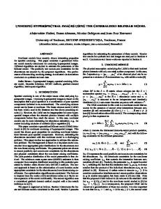
Fig. 1.2 shows the estimated distributions of Bayesian, linearization and subgradient). estimation of the nonlinearity parameter

b

for the images

I1 , . . . , I4

using the three presented algorithms (i.e.,

This gure shows that the three algorithms perform similarly for the

b.

Figure 1.2: Histograms of the estimated nonlinearity parameter ˆb for the four synthetic images estimated by the Bayesian (black), linearization-based (red) and subgradient-based (blue) algorithms.

30


Table 1.3 shows the execution times of MATLAB implementations on a 1.66GHz Dual-Core of the proposed algorithms for unmixing the proposed images (2500 pixels for each image). The linearization-based algorithm has the lowest computational cost and also provides accurate estimations.

Note that the computational cost of the

Bayesian algorithm (which allows prior knowledge to be included in the unmixing procedure) can be prohibitive for larger images and a high number of endmembers. However, the computational cost of the two proposed optimization methods (linearization and gradient-based) is very reasonable which make them very useful for practical applications.

Table 1.3: Computational times of the unmixing algorithms for 2500 pixels (in second). I1

I2

I3

I4

Bayesian

5960

6200

6600

5970

Taylor

5

10

8

7

Subgradient

84

102

96

101

The next set of simulations analyzes the performance of the proposed nonlinear SU algorithms for dierent numbers of endmembers (R

∈ {3, 6, 9, 12}) by unmixing 4 synthetic images of 500 pixels.

The endmembers contained in these

images have been randomly selected from the fourteen endmembers extracted by VCA from the full Cuprite scene described by Clark

et al.

(2003). For each image, the abundance vectors

an , (n = 1, . . . , 500)

have been randomly

generated according to a uniform distribution over the admissible set dened by the positivity and sum-to-one constraints. All images have been corrupted by an additive white Gaussian noise corresponding to a signal-to-noise ratio

SNR = 20dB.

The nonlinearity coecients

b

are uniformly drawn in the set

(−0.3, 0.3).

Table 1.4 compares

the performance of the three proposed methods in term of abundance estimation and reconstruction error. These results show that the three methods perform similarly in term of reconstruction error. The Bayesian estimators tend to provide more accurate abundance estimations (i.e., smaller RNMSEs) for large values of

R.

Indeed, the

Taylor and gradient algorithms may be trapped in local minima of the LS criterion (1.21) for large values of

Table 1.4: Unmixing performance of the supervised PPNMM-based algorithms for dierent R. −2

Average RNMSEs(×10 Bayesian

−2

AREs(×10

)

Taylor

Gradient

MMSE

MAP

R=3

7.50

10.42

9.43

R=6

7.53

11.37

R=9

5.69

R = 12

4.72

Bayesian

)

Taylor

Gradient

4.22

4.17

4.17

4.22

4.24

4.20

4.20

11.41

4.27

4.29

4.24

4.24

10.58

4.18

4.19

4.13

4.13

MMSE

MAP

9.41

4.18

12.65

12.16

9.56

11.90

8.08

11.16

31

R.


Real data The rst real image considered in this section is composed of

L = 189

spectral bands and was acquired in 1997 by

the airborne visible infrared imaging spectrometer (AVIRIS) over the Cuprite mining site in Nevada. A sub-image of size

50 × 50

pixels has been chosen here to evaluate the proposed unmixing procedures.

The scene is mainly

composed of muscovite, alunite and kaolinite, as explained by Dobigeon et al. (2009a). The endmembers extracted by VCA (Nascimento and Bioucas-Dias, 2005) and the nonlinear EEA proposed by Heylen et al. (2011) (referred to as Heylen"), with

R=3

are depicted in Fig. 1.3. The endmembers obtained by the two methods have similar

shapes. This result conrms the fact that the geometric EEAs (such as VCA) can be used as a rst approximation for endmember estimation (Keshava and Mustard, 2002).

Figure 1.3: The R = 3 endmembers estimated by VCA (blue lines) and Heylen (red lines) for the Cuprite scene. The three estimation algorithms presented above have been applied independently to each pixel of the scene using the endmembers extracted by the two EEAs. Examples of abundance maps obtained by the Heylen's method are presented in Fig. 1.4. They are similar to the abundance maps obtained with the FCLS algorithm which relies on the LMM. However, the advantage of the PPNMM is that it allows the nonlinearities between the observations and the abundance vectors to be analyzed. For instance, Fig. 1.5 shows the estimated maps of

b

for the Cuprite image.

These results show that the observations are nonlinearly related to the endmembers (since nonlinearity is weak since the estimated values of

b

are close to 0.

32

b 6= 0).

However, the


Figure 1.4: Abundance maps estimated by the Bayesian, linearization and subgradient methods for the Cuprite scene.

Figure 1.5: Maps of the nonlinearity parameter b estimated by the Bayesian, linearization and subgradient methods for the Cuprite scene. The second real image considered in this section is composed of

L = 189

by the satellite AVIRIS over the Moett Field, CA. A sub-image of size

spectral bands and was acquired in 1997

50 × 50

pixels has also been chosen here

to evaluate the proposed unmixing procedures. The scene is mainly composed of water, vegetation and soil. The endmembers extracted by VCA and Heylen's method with

33

R=3

are depicted in Fig. 1.6. Again, the endmembers


obtained by the two methods are similar.

Examples of abundance maps estimated by the proposed algorithms

with Heylen's method are presented in Fig. 1.7. They are similar to the abundance maps obtained with the FCLS algorithm which relies on the LMM. Fig. 1.8 shows the estimated maps of area, the observations are nonlinearly related to the endmembers (since

b

for the Moett image. In the water

b 6= 0).

These nonlinearities can be due to

the low amplitude of the water spectrum and nonlinear bathymetric eects.

Figure 1.6: The R = 3 endmembers estimated by VCA (blue lines) and Heylen (red lines) for the Moett scene. The quality of unmixing is nally evaluated using the AREs for both real images. These AREs are compared in Table 1.5 with those obtained by assuming other mixing models. The proposed PPNMM provides smaller AREs when compared to other models which is a very encouraging result.

Table 1.5: AREs (×10−2 ): Cuprite and Moett images VCA

LMM FM

GBM

PPNMM

Heylen

Cuprite

Moett

Cuprite

Moett


2.14

2.70

2.35

2.02


2.11

2.62

2.10

2.00

Bayesian

7.36

2.31

2.30

1.92


3.05

2.29

2.29

1.92


2.24

2.57

2.11

1.99


2.34

2.41

2.03

2.01


2.02

2.30

2.04

1.93

Bayesian

1.19

1.59

1.91

1.85

Taylor

1.19

1.54

1.90

1.84

Gradient

1.19

1.55

1.90

1.87

34


Figure 1.7: Abundance maps estimated by the Bayesian, linearization and subgradient methods for the Moett scene.

Figure 1.8: Maps of the nonlinearity parameter b estimated by the Bayesian, linearization and subgradient methods for the Moett scene.

35


1.4.4 Intermediate conclusion A Bayesian and two least squares algorithms were presented for supervised nonlinear SU of hyperspectral images. These algorithms assumed that the hyperspectral image pixels are related to the endmembers by a polynomial post-nonlinear mixing model. In the Bayesian framework, the constraints related to the unknown parameters were ensured by using appropriate prior distributions. was then derived.

The posterior distribution of the unknown parameter vector

The corresponding minimum mean square error estimator was approximated from samples

generated using Markov chain Monte Carlo methods. Least squares methods were also investigated for unmixing the polynomial post-nonlinear model.

These methods provided results similar to the Bayesian algorithm with a

reduced computational cost, making them very attractive for hyperspectral image unmixing. Results obtained on synthetic and real images illustrated the accuracy of the polynomial post-nonlinear model and the performance of the corresponding estimation algorithms for supervised unmixing. In this study, we assumed that the endmembers were known (either coming from

a priori

or extracted from the data using a EEA). However, as it has been shown

for linear SU, a joint estimation of the endmembers and mixing coecients can provide more accurate mixture characterization, especially when there is not enough pure pixels in the observed image. This joint estimation is the aim of the last part of this chapter which addresses the problem of unsupervised SU using the PPNMM. The next section generalizes the Bayesian model proposed for supervised nonlinear unmixing to the case where the endmembers are unknown and to be estimated. Least-squares methods could also have been investigated. However, their convergence is dicult to prove and the proposed Bayesian algorithm provides accurate results in practice. Including the endmembers in the estimation procedure complicates the unmixing procedure and estimating more parameters usually requires a higher computational cost. To improve the mixing properties and the complexity of the sampler, Hamiltonian Monte Carlo methods are investigated.

36


1.5

Unsupervised PPNMM-based unmixing

In this second scenario, the spectral signatures of the endmembers contained in the hyperspectral image are unknown and thus to be estimated. Only the number of endmembers is assumed to be known. Consider a hyperspectral image consisting of

N

pixels distributed according to (1.3). The PPNMM dened in (1.3) allows the

Y = [y1 , . . . , yN ]

matrix

L×N

observation

to be expressed as follows

Y = MA + [(MA) (MA)] diag (b) + E where

A = [a1 , . . . , aN ]

is an

R×N

matrix,

E = [e1 , . . . , eN ]

is an

L×N

(1.38)

matrix,

b = [b1 , . . . , bN ]T

is an

N ×1

en , ∀n ∈ {1, . . . , N } are additive 2 independently distributed zero-mean Gaussian vectors with diagonal covariance matrix Σ = diag σ , denoted as 2 T en ∼ N (0L , Σ), where σ 2 = [σ12 , . . . , σL ] is the vector of the L noise variances and diag σ 2 is an L × L diagonal vector containing the nonlinearity parameters. In this scenario, the noise sequences

matrix containing the elements of the vector

σ2 .

Note that this noise characterization is more general than the

one considered in the supervised SU scenario presented above. the

N

Precisely, the

N

noise vectors associated with

pixels have noise variances diering from one spectral band to another, which is in agreement with real

noise measurements. The abundance vectors in

A

satisfy the positivity and sum-to-one constraints (1.4) and the

endmembers to be estimated are subject to the constraints (1.5).

1.5.1 Bayesian estimation This section generalizes the hierarchical Bayesian model introduced in Section 1.4 in order to jointly estimate the abundances and endmembers, leading to a fully unsupervised hyperspectral unmixing algorithm.

To handle

abundance constraints, we propose to reparameterize the abundance vectors using the following transformation

r−1 Y

ar,n =

! zk,n

k=1

  1−z r,n ×  1

if

r 0

N

pixels, the Hammersley-Cliord theorem yields

N X X

1 exp β G(β) n=1

is the granularity coecient,

G(β)

 δ(zn − zn0 )

(4.14)

n0 ∈V(n)

is a normalizing (or partition) constant and

delta function. Several neighborhood structures can be employed to dene

V(n).

δ(·)

is the Dirac

Fig. 4.1 shows two examples of

neighborhood structures. The eight pixel structure (or 2-order neighborhood) will be considered in the rest of the chapter.

Figure 4.1: 4-pixel (left) and 8-pixel (right) neighborhood structures. The considered pixel appear as a black circle whereas its neighbors are depicted in white. The hyperparameter of

β

β

tunes the degree of homogeneity of each region in the image. More precisely, small values

yield an image with a large number of regions, whereas large values of

regions.

β

In this study, the granularity coecient is assumed to be known.

lead to fewer and larger homogeneous Note however that it could be also

included within the Bayesian model and estimated using the strategy described by Pereyra et al. (2013).

4.5.3 Hyperparameter priors The performance of the proposed Bayesian model for spectral unmixing mainly depends on the values of the hyperparameters

2 sk k=1,...,K .

When the hyperparameters are dicult to adjust, it is the norm to include them in

the unknown parameter vector, resulting in a hierarchical Bayesian model (Robert, 2007). This strategy requires the denition of prior distributions for the hyperparameters.

123

Chapter 4. Joint supervised unmixing and nonlinearity detection using residual component analysis

The following inverse-gamma prior distribution

s2k |γ, ν ∼ IG(γ, ν), is assigned to the nonlinearity hyperparameters, where a noninformative prior for

s2k ((γ, ν) = (1, 1/4)

∀k ∈ {1, . . . , K} (γ, ν)

(4.15)

are additional parameters that will be xed to ensure

in all simulations presented in this chapter).

Assuming prior

independence between the hyperparameters, we obtain

f (s2 |γ, ν) =

K−1 Y

f (s2k |γ, ν).

(4.16)

k=1 where

4.6

s2 = [s21 , . . . , s2K ]T .

Bayesian inference using a Metropolis-within-Gibbs sampler

4.6.1 Marginalized joint posterior distribution The resulting directed acyclic graph (DAG) associated with the proposed Bayesian model introduced in Sections 4.4 and 4.5 is depicted in Fig. 4.2.

γ

ν

s2

β

z

M

A

Φ

σ2

+' Y sw

Figure 4.2: DAG for the parameter and hyperparameter priors (the xed parameters appear in boxes). Assuming prior independence between

A, (Φ, z) and σ 2 , the posterior distribution of (Φ, θ) where θ = (C, z, σ 2 , s2 )

can be expressed as

f (θ, Φ|Y, M) ∝ f (Y|M, θ, Φ)f (Φ|M, z, s2 )f (θ), where

f (θ) = f (C)f (σ 2 )f (z)f (s2 ).

This distribution can be marginalized with respect to

Z f (θ|Y, M) ∝ f (θ) ∝

Φ

as follows

f (Y|M, θ, Φ)f (Φ|M, z, s2 )dΦ

f (θ)f (Y|M, θ)

(4.17)

where

Z f (Y|M, θ)

= ∝

f (Y|M, θ, Φ)f (Φ|M, z, s2 )dΦ

K−1 Y

Y

k=0 n∈Ik

1 T −1 ¯ Σ y ¯ 1 exp − y 2 n k n |Σk | 2

124

1

(4.18)


with

Σ0 =

diag

σ2

Σk = s2k KM + Σ0 (k = 1, . . . , K − 1)

,

marginalization is to avoid sampling the nonlinearity matrix

Φ.

and

¯ n = yn − Man . y

The advantage of this

Thus, the nonlinearities are fully characterized by

the known endmember matrix, the class labels and the values of the hyperparameters in

s2 = [s21 , . . . , s2K ]T .

Note

that the alternative interpretation of the proposed RCA-based model provided in Appendix H also leads to the

Φ

likelihood marginalized over

in (4.18).

Unfortunately, it is dicult to obtain closed form expressions for standard Bayesian estimators associated with (4.17). In this study, we propose to use ecient Markov Chain Monte Carlo (MCMC) methods to generate samples asymptotically distributed according to (4.17). is proposed to sample according to (4.17).

The next part of this section presents the Gibbs sampler which

The principle of the Gibbs sampler is to sample according to the

conditional distributions of the posterior of interest (Robert and Casella, 2004, Chap. 10). Due to the large number of parameters to be estimated, it makes sense to use a block Gibbs sampler to improve the convergence of the sampling procedure. More precisely, we propose to sample sequentially the

σ

the noise variances

2

and

2

s

N

labels in

z,

the abundance matrix

A,

using moves that are detailed in the next paragraphs.

4.6.2 Sampling the labels For the

nth

pixel (n

∈ {1, . . . , N }),

the label

zn

is a discrete random variable whose conditional distribution is fully

characterized by the probabilities

P (zn = k|yn , M, θ \zn ) ∝ f (yn |M, s2 , zn = k, an )f (zn |z\n ), where

θ \zn

zn , k = 0, . . . , K − 1 (for K classes). These posterior probabilities are   N X X 1 1 T −1   ¯ . ¯ Σ y P (zn = k|yn , M, θ \zn ) ∝ β δ(zp − zp0 ) exp − y 1 exp 2 n k n |Σk | 2 p=1 p0 ∈V(p)

denotes

θ

without

Consequently, sampling set

{0, . . . , K − 1}

(4.19)

zn

(4.20)

from its conditional distribution can be achieved by drawing a discrete value in the nite

with the probabilities dened in (4.20).

4.6.3 Sampling the abundance matrix A Sampling from

f (C|Y, M, z, σ 2 , s2 )

seems dicult due to the complexity of this distribution. However, it can be

shown that

f (C|Y, M, z, σ 2 , s2 ) =

N Y

f (cn |yn , M, zn , σ 2 , s2 ),

(4.21)

n=1 i.e., the

N

abundance vectors

{an }n=1,...,N

are a posteriori independent and can be sampled independently in a

parallel manner. Straightforward computations lead to

cn |yn , M, zn = k, σ 2 , s2 ∼ NS (¯ cn , Ψ n )

(4.22)

where

Ψn ¯n c

=

−1 f T Σ−1 M f M k

f T Σ−1 y = Ψn M k ˜n

f = M

[m1 − mR , . . . , mR−1 − mR ]

125

(4.23)


and

˜ n = yn − mR . y

simplex

S

Moreover,

with hidden mean

NS (¯ cn , Ψn ) denotes the truncated multivariate Gaussian distribution dened on the

¯n c

and hidden covariance matrix

Ψn .

Sampling from (4.22) can be achieved eciently

using the method recently proposed by Pakman and Paninski (2012).

4.6.4 Sampling the noise variance σ2 It can be shown from (4.17) that

f (σ 2 |Y, M, A, z, s2 ) =

L Y

f (σ`2 |Y, M, A, z, s2 ),

(4.24)

`=1 where

f (σ`2 |Y, M, A, z, s2 )

K−1 1 T −1 1 Y Y 1 2 ¯ ¯ ∝ 2 . 1 exp − y n Σk y n 1R+ σ` σ` 2 |Σk | 2 k=0 n∈Ik

(4.25)

Sampling from (4.25) is not straightforward. In this case, an accept/reject procedure can be used to update

σ`2 ,

leading to a hybrid Metropolis-within-Gibbs sampler. In this study, we introduce the standard change of variables

δ` = log(σ`2 ), δ` ∈ R.

A Gaussian random walk for

δ`

is used to update the variance

σ`2 .

This change of variables

allows the proposals to be symmetric, conversely to the truncated Gaussian distribution.

Note that the noise

2 variances σ` are a posteriori independent. Thus they can be updated in a parallel manner. The variances of the

L

parallel Gaussian random walk procedures have been adjusted during the burn-in period of the sampler to obtain an acceptance rate close to

0.5,

as recommended in (Robert and Cellier, 1998, p. 8).

4.6.5 Sampling the vector s2 It can be shown from (4.17) that

f (s2 |Y, M, A, z, σ 2 , γ, ν) =

K−1 Y

f (s2k |Y, M, A, σ 2 , γ, ν),

k=1 where

f (s2k |Y, M, A, σ 2 , γ, ν) ∝ f (s2k |γ, ν)

Y n∈Ik

1 T −1 ¯ ¯ exp − y Σ y . 1 2 n k n |Σk | 2 1

(4.26)

Due to the complexity of the conditional distribution (4.26), Gaussian random walk procedures are used in the logspace to update the hyperparameters

{s2k }k=1,...,K−1

in a parallel manner (similarly to the noise variance updates).

Again, the proposal variances are adjusted during the burn-in period of the sampler. After generating

NMC

samples using the procedures detailed above and removing

Nbi

iterations associated with

the burn-in period of the sampler (Nbi has been set from preliminary runs), the marginal maximum a posteriori (MAP) estimator of the label vector, denoted as

ˆMAP , z

can be computed.

used to compute the minimum mean square error (MMSE) of variances and the hyperparameters samples (MMSE estimates).

{s2k }k=1,...,K−1

A

The label vector estimator is then

conditioned upon

ˆMAP . z=z

Finally, the noise

are estimated using the empirical averages of the generated

The next section studies the performance of the proposed algorithm for synthetic

hyperspectral images.

126


4.7

Simulations for synthetic data

4.7.1 First scenario: RCA vs. linear unmixing The performance of the proposed joint nonlinear SU and nonlinearity detection algorithm is rst evaluated by unmixing a synthetic image of

60 × 60

pixels generated according to the model (4.1).

The

R = 3

contained in these images (i.e., green grass, olive green paint and galvanized steel metal) have

endmembers

L = 207

dierent

spectral bands and have been extracted from the spectral libraries provided with the ENVI software (RSI (Research Systems Inc.), 2003) . The number of classes has been set to pixels. The hyperparameters

2 sk k=1,...,3

K = 4,

i.e,

K−1 = 3

classes of nonlinearly mixed

have been xed as shown in Table 4.2, which represents three possible

levels of nonlinearity. For each class, the nonlinear terms have been generated according to (4.11). The label map generated with

β = 1.2

is shown in Fig. 4.3 (left). The abundance vectors

an , n = 1, . . . , 3600

have been randomly

generated according to a uniform distribution over the admissible set dened by the positivity and sum-to-one constraints. The noise variance (depicted in Fig. 4.4 as a function of the spectral bands) have been arbitrarily xed using

σ`2 = 10−4 2 − sin π to model a non-i.i.d.

(colored) noise.

` L−1

.

(4.27)

The joint nonlinear SU and nonlinearity detection algorithm, denoted as

RCA-SU, has been applied to this data set with

NMC = 3000

and

Nbi = 1000.

Fig. 4.3 (right) shows that the

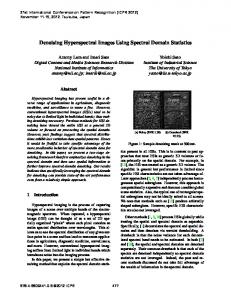
estimated label map (marginal MAP estimates) is in agreement with the actual label map. Moreover, the confusion matrix depicted in Table 4.1 illustrate the performance of the RCA-SU in term of pixel classication. Table 4.2 shows that the RCA-SU provides accurate hyperparameter estimates and thus can be used to obtain information about the importance of nonlinearities in the dierent regions. Note that the estimation error is computed using

|s2k − sˆ2k |/s2k ,

where

s2k

and

sˆ2k

are the actual and estimated dispersion parameters for the

noise variances, depicted in Fig.

k th

class. The estimated

4.4 are also in good agreement with the actual values of the variances.

The

Figure 4.3: Actual (left) and estimated (right) classication maps of the synthetic image associated with the rst scenario.

127


Figure 4.4: Actual noise variances (red) and variances estimated by the RCA-SU algorithm (blue) for the synthetic image associated with the rst scenario.

quality of abundance estimation can be evaluated by comparing the estimated and actual abundance vectors using the root normalized mean square error (RNMSE) dened in each class by

s RNMSEk

=

1 X 2 kˆ an − an k Nk R

(4.28)

n∈Ik

with

Nk = card(Ik )

and where

an

and

ˆn a

are the actual and estimated abundance vectors for the

nth

pixel of the

image. For this scenario, the proposed algorithm is compared with the classical FCLS algorithm (Heinz and C.-I Chang, 2001) assuming the LMM. Comparisons to nonlinear SU methods will be addressed in the next paragraph (scenario 2). Table 4.3 shows the RNMSEs obtained with the proposed and the FLCS algorithms for this rst data set. These results show that the two algorithms provide similar abundance estimates for the rst class, corresponding to linearly mixed pixels. For the three nonlinear classes, the proposed algorithm provides better results than the FCLS algorithm that does not handle nonlinear eects.

Table 4.1: First scenario: Confusion matrix (N = 3600 pixels). Estimated classes

Actual classes

C0

C1

C2

C3

C0

659

0

0

0

C1

1

1274

2

0

C2

0

4

787

2

C3

0

0

0

871

128


Table 4.2: First scenario: Hyperparameter estimation. s21

s22

s23

Actual value

0.01

0.1

1

Estimation error

2.76%

1.12%

0.28%

Table 4.3: RNMSEs (×10−2 ): synthetic images . Class #0

Class #1

Class #2

Class #3

FCLS

0.38

15.23

29.95

42.79

RCA-SU

0.38

2.83

3.99

4.23

4.7.2 Second scenario: RCA vs. nonlinear unmixing

Data set

The performance of the proposed joint nonlinear SU and nonlinearity detection algorithm is then evaluated on a second synthetic image of

60×60 pixels containing the R = 3 spectral components presented in the previous section.

In this scenario, the image consists of pixels generated according to four dierent mixing models associated with four classes (K

= 4).

The label map generated using

with the LMM. The pixels of class

yn

C1

=

n ∈ I1

is shown in Fig. 4.5 (a). The class

C0

is associated

have been generated according to the GBM (Halimi et al., 2011a)

R X

ar,n mr +

r=1 where

β = 1.2

and the nonlinearity parameters

R−1 X

R X

γi,j ai,n aj,n mi mj + en

(4.29)

i=1 j=i+1

{γi,j } have been uniformly drawn in [0.5, 1].

The class

C2

is composed

of pixels generated according to the PPNMM introduced in Chapter 1 as follows

yn =

R X r=1

where with

n ∈ I2 2

s = 0.1.

and

b = 0.5

ar,n mr + b

R X

!

ar,n mr

r=1

for all pixels in class

C2 .

R X

! ar,n mr

+ en

Finally, the class

C3

has been generated according to (4.1)

For the four classes, the abundance vectors have been randomly generated according to a uniform

distribution over the admissible set dened by the positivity and sum-to-one constraints. corrupted by an additive i.i.d Gaussian noise of variance ratio

(4.30)

r=1

SNR ' 30dB.

The noise is assumed to be i.i.d.

2

σ = 10

−4

All pixels have been

, corresponding to an average signal-to-noise

for a fair comparison with SU algorithms assuming i.i.d.

Gaussian noise. Fig. 4.5 (b) shows the log-energy of the nonlinearity parameters for each pixel of the image, i.e.,

2 log kφn k

for

n = 1, . . . , 3600.

This gure shows that each class corresponds to a dierent level of nonlinearity.

Unmixing Dierent estimation procedures have been considered for the four dierent mixing models:

•

The FCLS algorithm (Heinz and C.-I Chang, 2001) which is known to have good performance for linear mixtures.

•

The GBM-based approach (Halimi et al., 2011b) which is particularly adapted for bilinear nonlinearities.

129


(a) Actual label map.

(b) log kφn k2 .

(c) Detection map (PPNMM).

(d) Detection map (RCA-SU).

Figure 4.5: Nonlinearity detection for the scenario #2. •

The gradient-based approach introduced in Chapter 1 which is based on a PPNMM.

•

The proposed RCA-SU algorithm which has been designed for the model in (4.1). It has been applied to this data set with

•

NMC = 3000, Nbi = 2000, K = 4

and

β = 1.2.

Finally, we consider the K-Hype method studied by Chen et al. (2013b) to compare our algorithm with state-of-the art kernel based unmixing methods.

The kernel used in this study is the polynomial, second

order symmetric kernel whose Gram matrix is dened by (4.12).

This kernel provides better performance

on this data set than the kernels studied by Chen et al. (2013b) (namely the Gaussian and the polynomial, second order asymmetric kernels). All hyperparameters of the K-Hype algorithm have been optimized using preliminary runs.

Table 4.4 compares the RNMSEs obtained with the SU algorithms for each class of the second scenario.

These

results show that the proposed algorithm provides abundance estimates similar to those obtained with the LMMbased algorithm (FCLS) for linearly mixed pixels.

Moreover, the RCA-SU also provides accurate estimates for

130


the three mixing models considered, which illustrates the robustness of the RCA-based model regarding model mis-specication.

Table 4.4: Abundance RNMSEs (×10−2 ): Scenario #2 . Class #0

Class #1

Class #2

Class #3

(LMM)

(GBM)

(PPNMM)

(RCA)

FCLS

0.35

9.20

19.74

30.73

GBM

0.36

3.05

15.24

29.53

PPNMM

0.65

1.37

0.48

23.77

K-HYPE

3.24

3.28

3.14

3.42

RCA-SU

0.35

1.58

2.14

3.41

Unmixing algo.

The unmixing quality is also evaluated by the reconstruction error (RE) dened as

s REk

=

1 X 2 kˆ yn − yn k Nk L

(4.31)

n∈Ik

where

yn

is the

nth

observation vector and

ˆn y

its estimate. Table 4.5 compares the REs obtained for the dierent

classes. This table shows the accuracy of the proposed model for tting the observations. The REs obtained with the RCA-SU are similar for the four pixel classes.

Moreover, the performance in terms of RE of the proposed

algorithm are similar to the performance of the K-Hype algorithm.

Table 4.5: REs (×10−2 ): Scenario #2. Class #0

Class #1

Class #2

Class #3

(LMM)

(GBM)

(PPNMM)

(RCA)

FCLS

0.99

2.17

1.33

3.10

GBM

1.00

1.12

4.41

10.98

PPNMM

0.99

1.01

0.99

3.80

K-HYPE

0.98

0.98

0.98

0.98

RCA-SU

1.00

0.98

0.98

0.98

Unmixing algo.

From a reconstruction point of view, the K-Hype and RCA-SU algorithms provides similar results. However, the proposed algorithm also provides nonlinearity detection maps.

The PPNMM and RCA-SU algorithms perform

similarly in term of abundance estimation and allow both nonlinearities to be detected in each pixel. However, the nonlinearities can be analyzed more deeply using the RCA-SU, as will be shown in the next part.

Nonlinearity detection The performance of the proposed algorithm for nonlinearity detection is compared to the detector studied in Chapter 3, which is coupled with the PPNMM-based SU procedure mentioned above. alarm of the PPNMM-based detection has been set to PFA

= 0.05.

Figs.

The probability of false

4.5 (c) and (d) show the detection

maps obtained with the two detectors. Both detectors are able to locate the nonlinearly mixed regions. However, the RCA-SU provides more homogeneous regions, due to the consideration of spatial structure through the MRF.

131


Moreover, the proposed algorithm provides information about the dierent levels of nonlinearity in the image thanks to the estimation of the hyperparameters obtain [ˆ s21 , sˆ22 , sˆ23 ]

C2

= [0.2, 1.4, 10] × 10

−2

s2k

associated with the dierent classes.

, showing that nonlinearities of class

that are themselves weaker than those of class

C3 .

C1

In this simulation, we

are less severe than those of class

The next section studies the performance of the proposed

algorithm for a real hyperspectral image.

4.8

Simulations for a real hyperspectral image

4.8.1 Data set The real image considered in this section is the Villelongue image considered in Chapters 1 and 2. A sub-image (of size

41 × 29

pixels) is chosen here to evaluate the proposed unmixing procedure and is depicted in Fig. 4.6. The

scene is composed mainly of roof, road and grass pixels, resulting in

R=3

endmembers. The spectral signatures of

these components have been extracted from the data using the N-FINDR algorithm (Winter, 1999) and are depicted in Fig. 4.7.

Figure 4.6: Real hyperspectral Madonna data acquired by the Hyspex hyperspectral scanner over Villelongue, France (left) and sub-image of interest (right).

4.8.2 Spectral unmixing The proposed algorithm has been applied to this data set with classes has been set to

K=4

(4.14) has been xed to

NMC = 3000

and

Nbi = 1000.

The number of

(one linear class and three nonlinear classes). The granularity parameter of the prior

β = 0.7.

Fig. 4.8 shows examples of abundance maps estimated by the FCLS algorithm,

the gradient-based method assuming the GBM, the PPNMM and the K-Hype (Chen et al., 2013b) algorithms and the proposed method. The abundance maps estimated by the RCA-SU algorithm are in good agreement with the state-of-the art algorithms. However, Table 4.6 shows that K-Hype and the proposed algorithm provide a lower reconstruction error. Fig. 4.9 compares the noise variances estimated by the RCA-SU for the real image with the noise variances estimated by the HySime algorithm (Bioucas-Dias and Nascimento, 2008). The HySime algorithm

132


Figure 4.7: The R = 3 endmembers estimated by N-Findr for the real Madonna sub-image. assumes additive noise and estimates the noise covariance matrix of the image using multiple regression. Fig. 4.9 shows that the two algorithms provide similar noise variance estimates. These results motivate the consideration of non i.i.d. noise for hyperspectral image analysis since the noise variances increase for the highest wavelengths. The simulations conducted on this real dataset show the accuracy of the proposed RCA-SU in terms of abundance estimation and reconstruction error, especially for applications where the noise variances vary depending on the wavelength. Moreover, it also provides information about the nonlinearities of the scene.

Table 4.6: Reconstruction errors: Real image. Unmixing algo.

RE (×10−2 )

FCLS

0.65

GBM

0.65

PPNMM

0.54

K-HYPE

0.48

RCA-SU

0.48

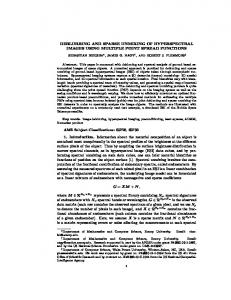
4.8.3 Nonlinearity detection Fig. 4.10 (b) shows the detection map (map of for the real image considered.

zn

for

n = 1, . . . , N )

provided by the proposed RCA-SU detector

Due to the consideration of spatial structures, the proposed detector provides

homogeneous regions. Similar structures can be identied in this detection map and the true color image of the scene (Fig. 4.10 (a)). The estimated class the roof region. The class

C1

C0

(black pixels) associated with linearly mixed pixels is mainly located in

(dark grey pixels) can be related to regions where the main component in the pixels are

grass or road. Mixed pixels composed of grass and road are gathered in class

C2 (light grey pixels).

pixels located between the roof and the road are associated with the last class RCA-SU can identify three levels of nonlinearity, corresponding to nonlinearity class is class

C3 ,

C3

(white pixels). Moreover, the

[ˆ s21 , sˆ22 , sˆ23 ] = [0.03, 0.50, 29.5].

The most inuent

C2

contain weaker nonlinearities.

C1 are associated with the weakest nonlinearities.

The nonlinearities of this class

where shadowing eects occurs. Mixed pixels of class

Finally, the remaining pixels of class

Finally, shadowed

133


Figure 4.8: The R = 3 abundance maps estimated by the FCLS, PPNMM-based, K-Hype, and RCA-SU algorithms for the Madonna real image (white pixels correspond to large abundances, contrary to black pixels).

134


Figure 4.9: Noise variances estimated by the RCA-SU (red) and the Hysime algorithm (blue) for the real Madonna image. can probably be explained by the endmember variability and/or the endmember estimation error. It is interesting to note that the RCA-SU identies two rather linear classes associated with homogeneous regions mainly composed of a single parameter (classes

C0

and

C1 ).

The two latter classes (classes

C2

and

C3 )

correspond to rather nonlinear

regions where the pixels are mixed and shadowing eects occur.

4.9

Conclusion

We have proposed a new hierarchical Bayesian algorithm for joint linear/nonlinear spectral unmixing of hyperspectral images and nonlinearity detection. This algorithm assumed that each pixel of the image is a linear or nonlinear mixture of endmembers contaminated by additive Gaussian noise. The nonlinear mixtures are decomposed into a linear combination of the endmembers and an additive term representing the nonlinear eects. A Markov random eld was introduced to promote spatial structures in the image. The image was decomposed into regions or classes where the nonlinearities share the same statistical properties, each class being associated with a level of nonlinearity. Nonlinearities within a same class were modeled using a Gaussian process parameterized by the endmembers and the nonlinearity level. Note nally that the physical constraints for the abundances were included in the Bayesian framework through appropriate prior distributions. Due to the complexity of the resulting joint posterior distribution, a Markov chain Monte Carlo method was investigated to compute Bayesian estimators of the unknown model parameters. Simulations conducted on synthetic data illustrated the performance of the proposed algorithm for linear and nonlinear spectral unmixing.

An important advantage of the proposed algorithm is its robustness regarding the

actual underlying mixing model. Another interesting property resulting from the nonlinear mixing model considered is the possibility of detecting several kinds of linearly and nonlinearly mixed pixels. This detection can be used to identify the image regions aected by nonlinearities in order to characterize the nonlinear eects more deeply. Finally, simulations conducted with real data showed the accuracy of the proposed unmixing and nonlinearity

135


(a)

(b)

Figure 4.10: (a) True color image of the scene of interest. (b) Nonlinearity detection map obtained with the RCA-SU detector for the Madonna image. detection strategy for the analysis of real hyperspectral images. As in Chapter 3, the endmembers contained in the hyperspectral image were assumed to be known in this work. Of course, the performance of the algorithm relies on this endmember knowledge. We think that estimating the pure component spectra present in the image, jointly with the abundance estimation and the nonlinearity detection is an important issue that should be considered in future work. Finally, the number of classes and the granularity of the scene were assumed to be known in this study. Estimating these parameters is clearly a challenging issue that should be investigated.

Main contributions.

A new nonlinear mixing model for joint hyperspectral image unmixing and nonlinearity

detection was proposed. The observed image was segmented into regions where nonlinear terms, if present, shared similar statistical properties.

The resulting algorithm provided accurate abundance estimates when the actual

mixtures are linear and nonlinear and it thus generalized the binary nonlinearity detectors proposed in the third chapter by considering dierent levels (classes) of nonlinearities.

136


4.10

Conclusion (in French)

Nous avons proposé un nouvel algorithme bayésien hiérarchique pour eectuer conjointement l'étape d'inversion et la détection de non-linéarités. Cet algorithme suppose que chaque pixel de l'image est un mélange linéaire ou non-linéaire des signatures spectrales des composants purs de l'image, contaminé par un bruit additif gaussien. Les mélanges non-linéaires sont décomposés en une combinaison linéaire des signatures spectrales des composants purs et d'un terme additif représentant les eets non-linéaires. Un champ de Potts-Markov a été introduit an de promouvoir les structures spatiales dans l'image. L'image a été décomposée en régions (ou classes) où les non-linéarités ont les mêmes propriétés statistiques, chaque classe étant associée à un niveau de non-linéarité. Les non-linéarités dans une même classe ont été modélisés en utilisant un processus gaussien paramétré par les composants de l'image et un niveau de non-linéarité. Les contraintes physiques sur les abondances ont également été incluses dans le cadre bayésien à l'aide de lois

a priori

appropriées. En raison de la complexité de la loi

a posteriori

jointe résultante, une

méthode MCMC a été utilisée pour calculer les estimateurs bayésiens des paramètres inconnus du modèle. Les simulations eectuées sur des données synthétiques ont illustré les performances de l'algorithme proposé pour résoudre le problème de démélange spectral linéaire et non linéaire. Un avantage important de l'algorithme proposé est sa robustesse vis-à-vis du modèle de mélange réel sous-jacent.

Une autre propriété intéressante résultant du

modèle de mélange non-linéaire considéré est la possibilité de détecter plusieurs types de pixels résultant de mélanges non-linéaires. Cette détection peut être utilisée pour identier les régions d'image aectées par des non-linéarités diérentes dans le but de caractériser plus nement les eets non-linéaires. Enn, les simulations eectuées avec des données réelles ont montré la pertinence des méthodes permettant d'eectuer conjointement l'étape d'inversion et la détection de non-linéarités pour l'analyse d'images réelles. Comme dans le chapitre 3, les composantes spectrales pures contenues dans l'image hyperspectrale ont été supposées connues dans ce chapitre. Bien sûr, les performances de l'algorithme sont liées à la connaissance de ces spectres. Dans le futur, il serait important de proposer des méthodes permettant de résoudre conjointement le problème de démélange non-supervisé et la détection de non-linéarités. Enn, le nombre de classes et la granularité de la scène ont également été supposés connus dans ce travail.

L'estimation de ces paramètres est clairement une question

dicile qui devrait être étudiée.

Contributions majeures.

Un nouveau modèle de mélange non-linéaire pour eectuer conjointement l'étape

d'inversion et la détection de non-linéarités a été proposée.

L'image observée a été segmentée en régions où les

termes non-linéaires, le cas échéant, partagent des propriétés statistiques similaires. L'algorithme résultant a fourni des abondances estimées satisfaisantes quand les mélanges réels sont linéaires et non linéaires et permet également de généraliser les détecteurs de non-linéarités binaires proposés dans le troisième chapitre de ce manuscrit en considérant diérents niveaux (classes) de non-linéarités.

137


138

Conclusion and future work The aim of this thesis was to study new nonlinear mixing models and to propose associated unmixing algorithms for hyperspectral image analysis. Spectral unmixing consists of extracting from a hyperspectral image, the spectra of the pure macroscopic components present in the image, referred to as endmembers, and of identifying their interactions referred to as mixtures.

To reduce the problem complexity, most works of the literature rely on a

linear mixing model, often considered as a rst approximation of the actual mixture. However, this approximation can be inaccurate to describe some scenes, requiring more complex mixing models to be considered (to overcome the inherent limitations of the linear model). Designing and/or choosing an appropriate nonlinear mixing model for spectral unmixing is a challenging problem because of the diversity of nonlinear eects. Moreover, introducing nonlinear terms in the observation model complicates the derivation of ecient nonlinear unmixing procedures relying on nonlinear models. Considering nonlinear eects in hyperspectral images usually require more complex unmixing strategies than those assuming linear mixtures.

Since the linear mixing model is often sucient to

approximate accurately most actual mixtures, it is also interesting to detect pixels or regions where the linear model is accurate.

4.11

Conclusion

The rst chapter studied a post-nonlinear mixing model (PNMM) for nonlinear SU. The proposed polynomial PNMM (PPNMM) investigated in this chapter allowed nonlinearities to dier for each pixel, leading to a exible mixture characterization.

The nonlinearity of each pixel was characterized by a single parameter which is zero

when the pixel is linearly mixed.

First, supervised SU methods based on the PPNMM were considered.

rst proposed algorithm was a hierarchical Bayesian algorithm coupled with MCMC methods.

The

Two alternative

optimization methods were also introduced to reduce the computational complexity of the sampling algorithm. The exibility of the PPNMM and the performance of the three methods were evaluated using simulations conducted on synthetic and real data. The second part of this chapter presented a new Bayesian model for unsupervised SU based on the PPNMM. Appropriate priors were also assigned to the unknown endmembers to be sampled. The joint estimation of the abundances and endmembers required a large number of parameters to be sampled. To improve the mixing properties of the sampler, constrained Hamiltonian Monte Carlo methods were investigated. The second chapter of this manuscript considered a kernel-based approach for nonlinear SU based on a nonlinear dimensionality reduction using a GPLVM. GPLVMs, which have received growing interest in the machine learning community, have the ability to approximate various nonlinear mappings from a low-dimensional space (latent space) to a higher dimensional observation space through the use of kernel functions, which makes them particularly well

139


adapted for hyperspectral image analysis and thus unmixing.

In this chapter, we proposed to use a particular

form of kernel based on existing bilinear models, which allowed the proposed unmixing strategy to be accurate when the underlying mixing model is bilinear.

The proposed unmixing algorithm breaks the usual paradigm of

spectral unmixing by rst estimating the abundances and then predicting the endmembers using GPs. Simulations conducted on synthetic and real images illustrated the exibility of the proposed model for linear and nonlinear spectral unmixing and provided promising results for abundance and endmember estimations even in the absence of pure pixels in the image. The third chapter of this manuscript was dedicated to the detection of nonlinearities in hyperspectral images. This chapter focused on supervised detection procedures, i.e., the endmembers were assumed to be

a priori

known. The

rst detector was based on the PPNMM studied in the rst chapter. More precisely, the associated test was based on the statistical properties of the PPNMM parameters to decide whether a given pixel is linearly or nonlinearly mixed. Conversely, the second test proposed did not assume any particular NLMM, i.e., only relied on the LMM. The two detectors were compared using simulations conducted on synthetic and real data. In the last chapter of this manuscript, a new nonlinear mixing model for joint hyperspectral image unmixing and nonlinearity detection was proposed.

The observed image was segmented into regions where nonlinear terms, if

present, shared similar statistical properties. The resulting algorithm provided accurate abundance estimates for linear and nonlinear mixtures. Thus, it generalized the binary nonlinearity detectors proposed in the third chapter by considering dierent classes (levels) of nonlinearities. In this manuscript, it was shown that nonlinear unmixing algorithms can improve the characterization of hyperspectral images compared to methods based on a linear model. These methods allowed the reconstruction errors to be reduced. Moreover, these methods provided better spectral signature and abundance estimates when the observed pixels result from nonlinear mixtures. The simulation results conducted on synthetic and real images illustrated the advantage of using nonlinearity detectors for hyperspectral image analysis. In particular, the proposed detectors can identify components which are present in few pixels (and hardly distinguishable) and can locate areas where signicant nonlinear eects occur (shadow, relief, ...).

4.12

Future work

In this manuscript, we proposed nonlinear unmixing and nonlinearity detection algorithms using a polynomial post-nonlinear model. The exibility of the Bayesian framework allowed the model complexity to be handled and prior information about the model parameters to be easily included within the estimation procedure. It would be interesting to extend this work to physics-based nonlinear models of the literature such as polynomial (bilinear) (Halimi et al., 2011a; Meganem et al., 2013) and intimate mixture models (Hapke, 1981). Consider the following bilinear model

yn =

R X

ar,n mr +

r=1

R−1 X

R X

βi,j,n mi mj + en

dened in (3). As mentioned in Chapter 4, the interaction spectra the estimation of the nonlinearity parameters

(4.32)

i=1 j=i+1

βi,j,n ,

mi mj

are highly correlated which complicates

especially for large numbers of endmembers

we considered such parameters as nuisance parameters which were marginalized.

140

R.

In Chapter 4,

However, if one is particularly


interested in these parameters (to quantify the inuence of each interaction), additional information should be included in the estimation procedure. expected to be small (or even null).

As mentioned by Gader et al. (2012), most of the

βi,j,n

parameters are

Consequently, it is interesting to enforce small values and/or sparsity for

these unknown parameters. In the Bayesian framework, sparsity promoting prior distributions (such as Laplace, Bernoulli-Gaussian or Bernoulli-Laplace distributions) could be used to infer the nonlinearity parameters. Even if the consideration of nonlinear terms increases the unmixing complexity, the recent advances in ecient simulation methods (including Hamiltonian Monte Carlo methods) for high dimensional problems are promising and their application to hyperspectral analysis is an interesting prospect. The second chapter of this manuscript focused on a kernel-based nonlinear dimensionality reduction technique initially studied in the machine learning community. A particular nonlinear mapping adapted for modeling bilinear nonlinearities was used and provided encouraging results. Moreover, the fourth chapter of this manuscript focused on a kernel-based model for joint unmixing and nonlinearity detection.

Kernel-based methods for hyperspectral

unmixing have recently received growing interest (Broadwater and Banerjee, 2009; Chen et al., 2013b) for their exibility. However, further eorts should be achieved for proposing more general but accurate kernel functions. In the fourth chapter of this manuscript, the nonlinearity of each pixel was characterized by a kernel function which only depends on the endmember matrix. However, it makes sense to assume that the nonlinearity may also depend on the pixel composition, i.e., on its abundances. Kernels depending on the endmembers and the abundances, such as in the kernel-based method recently proposed by Chen et al. (2013a), should be investigated. In the two last chapters of the manuscript, the endmembers were assumed to be known to perform the nonlinearity detection and the joint unmixing and nonlinearity detection.

However, if the endmembers are unknown, they

have to be extracted from the data, which can be dicult when nonlinearly mixed pixels are present in the scene. It would be interesting to apply nonlinearity detectors before the endmember extraction (and then using linear EEAs to identify the pure spectral signatures) or to propose joint nonlinearity detection and endmember estimation methods. Thus, it would be interesting to extend the RCA-based Bayesian model proposed in Chapter 4 to the case where the endmembers are included in the estimation procedure. In this manuscript, we considered linear and nonlinear mixing models whose parameters were estimated using Bayesian inference. Thus, the dimension of the unknown parameter vectors was known and thus their admissible sets were assumed to be unique. In particular, the number of endmembers

R

was xed from

a priori

knowledge.

In the RCA-based model, the number of classes was also xed. If the dimension of the unknown parameter vector is unknown, a simple solution consists of running the proposed algorithms with dierent numbers of endmembers and/or classes. However, the computational complexity of this approach can be prohibitive when the number of parameters to be tuned is large.

A more elegant approach consists of including the dimension of the unknown

parameter vector within the parameter estimation using the Bayesian framework.

Sampling from the resulting

posterior distribution can be achieved using reversible jump MCMC (RJ-MCMC) methods Green (1995).

RJ-

MCMC methods can be used for model order selection but also to sample variables that can live in disjoint sets, which is particularly interesting for hyperspectral image analysis. For instance, prior distributions dened on a set of (disjoint) domains could be assigned to unknown endmembers and/or abundances. As a toy example, consider the problem of semi-supervised unmixing of a hyperspectral image that consists of urban and forested areas. The problem is semi-supervised in the sense that the endmembers present in the image belong to a spectral library which contains spectra of both urban and forested areas. Instead of searching the active endmembers in the whole library,

141


it would be interesting to identify the urban and forested areas in the scene and to estimate the endmembers out of subsets of the library. For this problem, prior distributions for the unknown endmembers could be dened on dierent subsets of the library and RJ-MCMCs could be used to sample for the resulting posterior. This example is highly related to the sparse linear unmixing problem that have received intensive interest over the last few years in the hyperspectral community ((Bioucas-Dias et al., 2012) and references therein).

This sparse

linear regression problem has strong relations with compressed sensing and basis pursuit. It consists of solving the inversion step given a large spectral library by enforcing the abundances to be sparse. are mainly used to solve this problem and the the

`0

`1

Optimization algorithms

norm penalization is often preferred (`1 relaxation) rather than

norm, which is more challenging to handle. Conversely, the Bayesian framework is exible enough to handle

penalizations based on the

`0

norm, using RJ-MCMCs for instance.

Moreover, this framework allows also for

structured sparsity to be considered, such as in (Dobigeon and Févotte, 2013; Iordache et al., 2013).

Proposing

Bayesian sparse unmixing procedures is a very interesting prospect. However, ecient sampling procedures must be proposed to handle the complexity induced by the consideration of prior sparsity information. Finally, consideration of endmember variability for spectral unmixing is also interesting. In this manuscript, the spectral signatures of the materials of the scene were assumed to be unique. However, the spectral variability of these signatures cannot be neglected in some images. Solving the unmixing problem in such cases is challenging and should deserve deeper attention in future work.

142

Conclusion et perspectives (in French) L'objectif de cette thèse était d'étudier de nouveaux modèles de mélange non-linéaires et de proposer des algorithmes de démélange associés pour l'analyse d'images hyperspectrales.

Le problème de démélange spectral consiste à

extraire d'une image hyperspectrale, les spectres des composants macroscopiques purs présents dans l'image, et à idener leurs interactions ou mélanges. Pour réduire la complexité du problème, la plupart des travaux de la littérature s'appuient sur un modèle de mélange linéaire, souvent considéré comme une première approximation des mélanges réels.

Cependant, cette approximation peut ne pas être appropriée pour décrire certaines scènes

qui nécessitent d'utiliser des modèles de mélange plus complexes.

Dénir et/ou choisir un modèle de mélange

non-linéaire approprié pour le démélange spectral est un problème dicile en raison de la diversité des eets nonlinéaires. De plus, l'introduction de termes non-linéaires dans le modèle d'observation complique la mise en place de procédures de démélange ecaces reposant sur des modèles non-linéaires. Considérer des eets non-linéaires dans les images hyperspectrales exige habituellement des algorithmes de démélange plus complexes que ceux basés sur un modèle linéaire. Étant donné que le modèle de mélange linéaire est souvent susant pour modéliser avec précision la plupart des mélanges réels, il est aussi intéressant de détecter les pixels ou les régions où le modèle linéaire peut sure.

4.13

Conclusion

Dans le premier chapitre, nous avons étudié un modèle de mélange post-non-linéaire (PNMM) pour résoudre le problème de démélange non-linéaire. Le modèle proposé (PPNMM) étudié dans ce chapitre permet de considérer des non-linéarités diérentes pour les diérents pixels de l'image. La non-linéarité de chaque pixel est caractérisée par un paramètre unique qui est égal à zéro lorsque le pixel résulte d'un mélange linéaire.

Tout d'abord, des

méthodes de démélange supervisé basées sur le PPNMM ont été présentées. Le premier algorithme proposé est un algorithme bayésien hiérarchique couplée avec des méthodes MCMC. Deux méthodes d'optimisation alternatives ont également été introduites an de réduire le coût calculatoire de l'échantillonneur de Gibbs. La souplesse du PPNMM et les performances des trois méthodes ont été évaluées à l'aide de simulations eectuées sur données synthétiques et réelles. La deuxième partie de ce chapitre a présenté un nouveau modèle bayésien pour résoudre le problème de démélange non-supervisé. Des lois a priori appropriées ont été également attribuées aux signatures spectrales inconnues et à échantillonner. L'estimation conjointe des abondances et de ces signatures spectrales implique un grand nombre de paramètres à échantillonner. Pour améliorer les propriétés de mélange de l'échantillonneur, des méthodes de Monte Carlo à dynamiques hamiltoniennes contraintes ont été étudiées. Le second chapitre de ce manuscrit s'est focalisé sur une méthode à noyaux basée sur une réduction de dimension

143


non-linéaire utilisant un modèle à variables latentes et des processus gaussiens (GPLVM). Les GPLVMs, qui ont suscité un intérêt croissant dans la communauté de l'apprentissage automatique ont la capacité d'approcher à grand nombre d'applications non-linéaires d'un espace de faible dimension (espace latent) à un espace d'observation de dimension supérieure grâce à l'utilisation de noyaux, ce qui les rend particulièrement bien adaptés pour l'analyse d'images hyperspectrales et donc pour le démélange spectral. Dans ce chapitre, nous avons proposé d'utiliser une forme particulière de noyau basé sur des modèles bilinéaires existants, ce qui a permis d'obtenir un algorithme de démélange bien adapté lorsque le modèle de mélange sous-jacent est bilinéaire. L'algorithme de démélange proposée rompt le paradigme habituel du démélange spectral en estimant tout d'abord les abondances puis en prédisant les spectres de composants purs à l'aide de processus gaussiens. Les simulations eectuées sur des images synthétiques et réelles ont illustré la exibilité du modèle proposé pour le démélange linéaire et non-linéaire et ont donné des résultats prometteurs, même en l'absence de pixels purs dans l'image observée. Le troisième chapitre de ce manuscrit a été consacrée à la détection de non-linéarités dans les images hyperspectrales. Ce chapitre s'est concentré sur des procédures de détection supervisées dans le sens où les spectres des composants présents dans l'image étaient supposés connus. Le premier détecteur était fondé sur le modèle PPNMM étudié dans le premier chapitre. Plus précisément, le test proposé était basé sur les propriétés statistiques de l'estimateur du maximum de vraisemblance des paramètres du modèle PPNMM an de décider si un pixel résulte d'un mélange linéaire où non-linéaire. A contrario, le deuxième détecteur proposé ne supposait pas de formes de non-linéarités particulière, c'est-à-dire, ne reposait que sur le modèle de mélange linéaire. Les deux détecteurs ont été comparés à l'aide de simulations eectuées sur données synthétiques et réelles. Dans le dernier chapitre de ce manuscrit, un nouveau modèle de mélange non-linéaire pour eectuer conjointement le démélange supervisé et la détection de non-linéarités a été proposé. L'image observée a été segmentée en régions où les termes non-linéaires (lorsqu'ils sont présents) partagent des propriétés statistiques similaires. L'algorithme résultant a montré de bonnes performances en terme d'estimation des abondances lorsque les pixels de l'image résultent de mélange linéaires et non-linéaires. De plus, il généralise les détecteurs de non-linéarités binaires proposés dans le troisième chapitre en considérant diérentes classes (niveaux) de non-linéarités. Dans ce manuscrit, il a été montré que les algorithmes de démélange non-linéaires peuvent permettre d'améliorer la caractérisation des images hyperspectrales par rapport aux méthodes basées sur un modèle linéaire. Ces méthodes non-linéaires ont montré de bonnes performances en termes d'estimation des abondances lorsque les pixels de l'image résultent de mélange non-linéaires. Les résultats de simulations eectuées sur des images synthétiques et réelles ont illustré l'avantage de l'utilisation de détecteurs de non-linéarités pour l'analyse d'images hyperspectrales. En particulier, les détecteurs proposés permettent d'identier des composants très peu représentés (et dicile à détecter) et peuvent localiser des régions où se produisent des eets non-linéaires importants (ombre, relief, . . . ).

4.14

Perspectives

Dans ce manuscrit, nous avons proposé des algorithmes de détection de non-linéarités et de démélange non-linéaires en utilisant un modèle post-non-linéaire polynômial. La exibilité du cadre bayésien a permis de gérer la complexité du modèle à traiter et a également permis d'inclure facilement l'information disponible sur les paramètres du modèle dans la procédure d'estimation.

Il serait intéressant d'étendre ce travail à d'autres modèles non-linéaires de la

littérature, en particulier ceux motivés par les phénomènes physiques en jeu dans les processus de mélange (tels que

144


les modèles polynômiaux (Halimi et al., 2011a; Meganem et al., 2013) et les modèles de mélanges intimes (Hapke, 1981)). Considérons le modèle bilinéaire suivant

yn =

R X

ar,n mr +

r=1

R−1 X

R X

βi,j,n mi mj + en

(4.33)

i=1 j=i+1

déni par l'Eq. (3). Comme noté dans le chapitre 4, les spectres d'interactions complique l'estimation des paramètres de non-linéarité

mi mj

sont fortement corrélés, ce qui

βi,j,n , en particulier pour un grand nombre de composants R.

Dans le chapitre 4, nous avons considéré ces paramètres comme des paramètres de nuisance qui ont été marginalisés. Toutefois, si l'on est particulièrement intéressé par les valeurs de ces paramètres (si l'on veut quantier l'inuence de chaque interaction), de l'information supplémentaire doit être incluse dans la procédure d'estimation. Comme noté par Gader et al. (2012), on peut s'attendre à ce que les paramètres

βi,j,n

soient faibles (ou même nuls). Par

conséquent , il serait intéressant de promouvoir les faibles valeurs (voire la parcimonie) pour ces paramètres. Dans le cadre bayésien, des lois

a priori

favorisant la parcimonie (par exemple, des lois Laplace, Bernoulli-gaussienne ou

Bernoulli-Laplace) pourraient être utilisées pour estimer les paramètres de non-linéarité. Même si la considération de termes non-linéaires augmente la complexité du problème de démélange, les récents progrès dans le domaine des méthodes de simulation (y compris les méthodes de Monte Carlo à dynamiques hamiltoniennes) pour des problèmes de grande dimension sont prometteurs. Leur application à l'analyse d'images hyperspectrales est une perspective intéressante. Le deuxième chapitre de ce manuscrit a porté sur une technique de réduction de dimension à base de noyau étudiée à l'origine par la communauté de l'apprentissage automatique. Un noyau particulier et adapté aux non-linéarités bilinéaires a été utilisé et a fourni des résultats encourageants.

De plus, le quatrième chapitre de ce manuscrit

s'est focalisé sur un modèle à noyau pour eectuer conjointement le démélange et la détection de non-linéarités. Les méthodes à noyaux pour le démélange spectral ont récemment reçu un intérêt croissant, (Broadwater and Banerjee, 2009; Chen et al., 2013b) motivé par leur grande exibilité. Toutefois, des eorts supplémentaires doivent être réalisés pour proposer des noyaux plus généraux mais toujours adaptés à l'imagerie hyperspectrale. Dans le quatrième chapitre de ce manuscrit, la non-linéarité de chaque pixel était caractérisée par une fonction de noyau qui ne dépendait que de la matrice des signatures spectrales. Toutefois, il est raisonnable de penser que la nonlinéarité peut également dépendre de la composition de pixel, c'est-à-dire, de ses abondances. La modélisation des non-linéarités en utilisant les signatures spectrales pures et les abondances, comme dans la méthode récemment proposé par Chen et al. (2013a), est une perspective intéressante. Dans les deux derniers chapitres du manuscrit, les signatures spectrales des composants de l'image étaient supposées connues pour pourvoir eectuer la détection de non-linéarités et le démélange non-linéaire. Toutefois, si ces spectres sont inconnus, ils doivent être extraits des données, ce qui peut être dicile lorsque des pixels résultant de mélanges non-linéaires sont présents dans la scène.

Il serait intéressant d'appliquer des détecteurs de non-linéarités avant

l'extraction de ces signatures ou de proposer des méthodes réalisant conjointement l'estimation de ces spectres et la détection de non-linéarités. Par exemple, il serait intéressant d'étendre le modèle bayésien basé sur RCA proposé au chapitre 4 pour le cas où les signatures spectrales pures sont incluses dans la procédure d'estimation. Dans ce manuscrit, nous avons examiné des modèles de mélange linéaires et non-linéaires dont les paramètres étaient estimés par inférence bayésienne. De plus, la dimension des vecteurs de paramètres inconnus était connue et leurs ensembles de dénition étaient uniques. En particulier, le nombre de composants

145

R

était xé

a priori.

Dans


le modèle inspiré de RCA, le nombre de classes était également xé.

Si la dimension du vecteur de paramètres

inconnu est inconnue, une solution simple consiste à exécuter les algorithmes proposés avec diérents nombres de composants et/ou de classes.

Cependant, le coût calculatoire de cette approche peut être prohibitif lorsque

le nombre de paramètres à tester est important.

Une approche plus élégante consiste à inclure la dimension du

vecteur de paramètres inconnu dans la procédure d'estimation en utilisant le cadre bayésien. L'échantillonnage de la loi

a posteriori

qui en résulte peut être réalisé en utilisant des MCMC à sauts réversibles (RJ-MCMC) Green

(1995). Les méthodes de type RJ-MCMC peuvent être utilisées pour sélectionner l'ordre d'un modèle, mais aussi pour échantillonner des paramètres qui peuvent vivre dans des ensembles disjoints, ce qui est particulièrement intéressant pour l'analyse d'images hyperspectrales.

Par exemple, des lois

a priori

dénies sur un ensemble de

domaines (disjoints) peuvent être utilisées pour les signatures spectrales et/ou les abondances à estimer.

Un

exemple d'application pourrait être le problème de démélange semi-supervisé d'une image hyperspectrale qui se compose de zones urbaines et boisées. Le problème est semi-supervisé dans le sens où les composants présents dans l'image appartiennent à une bibliothèque spectrale qui contient les spectres des deux zones (urbaines et boisées). Au lieu de chercher les signatures spectrales actives dans l'ensemble de la bibliothèque, il serait intéressant d'identier les zones urbaines et boisées de la scène et de rechercher les signatures spectrales dans des sous-ensembles de la bibliothèque. Pour ce problème, des lois

a priori

pour les signatures spectrales inconnues pourraient être dénies

sur diérents sous-ensembles de la bibliothèque et des méthodes de type RJ-MCMC pourraient être utilisées pour échantillonner la loi

a posteriori

associée au modèle bayésien.

Cet exemple est fortement liée au problème de démélange linéaire parcimonieux qui a suscité un fort intérêt au cours des dernières années dans la communauté hyperspectrale (Bioucas-Dias et al., 2012). Ce problème consiste à résoudre l'étape d'inversion (estimation des abondances) à partir d'une large bibliothèque spectrale en forçant les abondances à être parcimonieuses. Des algorithmes d'optimisation sont souvent utilisés pour résoudre ce problème et la pénalisation par la norme

`1

est souvent préférée (relaxation par norme

`1 ) à la norme `0

qui est plus dicile à

manipuler. Inversement, le cadre bayésien est susamment souple pour gérer des pénalisations utilisant la norme

`0 ,

en utilisant des méthodes de type RJ- MCMC par exemple. De plus, ce cadre permet également de considérer des parcimonies structurées, comme dans (Dobigeon and Févotte, 2013; Iordache et al., 2013). Proposer les algorithmes bayésien de démélange parcimonieux est une perspective très intéressante. Toutefois, des échantillonneurs ecaces doivent être proposés pour gérer la complexité induite par la prise en compte de parcimonies. Enn, l'étude de la variabilité de signatures spectrales pour le démélange est également intéressante.

Dans ce

manuscrit, les signatures spectrales des matériaux de la scène étaient supposées être uniques. Cependant, la variabilité spectrale de ces signatures ne peut pas être négligée dans certaines images. Résoudre le problème de démélange dans de telles situations est dicile et ce cas devrait être approfondi dans le futur.

146

Appendices

147

Appendix A

Identiability of the supervised PPNMM-based SU problem A.1

Non-injectivity of s 7→ g(s)

The application

g:

[0, 1]L s

with

s = [s1 , . . . , sL ]T

which leads to

A.2 Let

2L

→ RL T 7→ s1 + bs21 , . . . , sL + bs2L

g(s1 ) = g(s2 ) then 1 ∀l = 1, . . . , L s2,i ∈ s1,i , − − s1,i b

is not injective. Indeed, if

solutions for the problem

g(s1 ) = g(s2 )

Injectivity of (a, b) 7→ g(a, b) = Ma + b(Ma) (Ma)

a and a∗ be two abundance vectors satisfying the positivity and sum-to-one constraints, M the matrix containing

the endmembers and

(b, b∗ ) ∈ R2 .

Consider the nonlinear functional

=

R X r=1

dened as follows

= Ma + b(Ma) (Ma)

g(a, b)

where

g(a, b)

ar mr + b

R X

a2r mr mr + 2b

r=1

R=1 X

R X

ar aj mr mj

r=1 j=r+1

denotes the term by term product operation. If

g(a, b) = g(a∗ , b∗ ),

then

M(a − a∗2 ) + b(Ma) (Ma) − b∗ (Ma∗ ) (Ma∗ ) = 0 and

R X r=1

(ar − a∗r )mr +

R X

(ba2r − b∗ a∗2 r )mr mr + 2

r=1

R=1 X

R X

r=1 j=r+1

149

(bar aj − b∗ a∗r a∗j )mr mj = 0.

Appendix A. Identiability of the supervised PPNMM-based SU problem

If the columns of the

L×

R(R+3) matrix 2

ˇ = {m1 , . . . , mR , m1 m1 , . . . , mR mR , m1 m2 , . . . , mR−1 mR } M are linearly independent, then

a = a∗ ,

and

b = b∗ .

(A.1)

ˇ Consequently, the identiability of the unmixing problem assuming the proposed PPNMM is ensured when rank(M) R(R+3) , which is usually satised when using real pure spectral components. 2

Note that the identiability of

the unmixing problem associated with the LMM requires a similar condition, i.e., rank(M)

T

[m1 , . . . , mR ]

.

150

=

= R,

where

M =

Appendix B

Partial derivatives for the LS PPNMM-based algorithms B.1

Partial derivatives of ˇ b(·) and h(·)

The partial derivative of

h(·)

with respect to

ar , (r = 1, . . . , R)

∂h(a) ∂ar

is given by

2 (Ma) mr .

=

Using the following partial derivatives

∂(y − Ma) ∂ar ∂(y − Ma)T h(a) ∂ar ∂h(a)T h(a) ∂ar

= −mr = −mTr h(a) + 2(y − Ma)T ((Ma) mr ) =

2h(a)T

∂h(a) ∂ar

and the usual dierentiation rules, we obtain

∂ ˇb(a) ∂ar

B.2

=

1 kh(a)k

4

∂(y − Ma)T h(a) ∂h(a)T h(a) T T h(a) h(a) − (y − Ma) h(a) . ∂ar ∂ar

ˇ ∗ (·) Partial derivatives of y

Thanks to the sum-to-one constraint of the abundance vector, the cost function (1.23) can be expressed as a function of

c = [a1 , . . . , aR−1 ]T

by setting

aR = 1 −

PR−1 r=1

ar .

Straightforward computations lead to

Ma = Mc + mR where

M , [m1 − mR , . . . , mR−1 − mR ] , [m1 , . . . , mR−1 ]

is a matrix of size

then be expressed as

∗ ˇ (c) = Mc + mR + ˇb (c)h(c) y

151

L × (R − 1).

The spectrum

ˇ (c) y

can

Appendix B. Partial derivatives for the LS PPNMM-based algorithms

where

ˇb ∗ (c)

= ˇb a1 , . . . , aR−1 , 1 −

R−1 X

! ar

r=1 and

h(c)

=

(Mc + mR ) (Mc + mR ).

Using the following partial derivatives with respect to

∂h(c) ∂cr ∂(y − Mc − mR ) ∂cr ∂(y − Mc − mR )T h(c) ∂cr ∂h(c)T h(c) ∂cr

=

cr

2mr Mc + mR

= −mr = −mTr h(c) + 2(y − Ma)T mr Mc + mR =

2h(c)T

∂h(c) ∂cr

and the usual dierentiation rules, we obtain

∗

∂ ˇb (c) ∂cr

= −

∂(y − Mc − mR )T h(c) h(c)T h(c) ∂cr ∂h(c)T h(c) T (y − Mc − mR ) h(c) . ∂cr 1

h(c) 4

Finally, the partial derivative of the estimated spectrum

ˇ ∗ (c) y

with respect to

∗ ˇ ∗ (c) ∂ ˇb (c) ∂h(c) ∂y ∗ = mr + h(c) + ˇb (c) . ∂cr ∂cr ∂cr

152

cr

is

Appendix C

Derivation of the potential functions associated the UPPNMM algorithm C.1

Derivation of the potential function associated with z n

The potential energy (1.61) can be rewritten

U (z n )

=

U1 (an ) + U2 (z n )

(C.1)

where

1 T [yn − gn (Man )] Σ−1 [yn − gn (Man )] , 2 R−1 X R−r−1 = − log zr,n .

U1 (an )

=

U2 (z n )

r=1


U (z n )

with respect to

zn

is obtained using the classical chain rule

∂U (z n ) ∂U1 (an ) ∂an ∂U2 (z n ) = + . ∂z n ∂an ∂z n ∂z n Straightforward computations lead to

∂U1 (an ) T = − [yn − gn (Man )] Σ−1 M + 2bn Man 1TR M ∂an

∂ar,n ∂zi,n ∂U2 (z n ) ∂zi,n

=

=

  0     ar,n zi,n − 1   ar,n    zi,n R−i−1 − . zi,n

153

if

i>r

if

i=r

if

i