Numerical Assessment of Cargo Liquefaction Potential. Lei Ju, Dracos Vassalos, Evangelos Boulougouris. Ship Stability Research Centre, Department of Naval ...
Numerical Assessment of Cargo Liquefaction Potential Lei Ju, Dracos Vassalos, Evangelos Boulougouris Ship Stability Research Centre, Department of Naval Architecture, Ocean & Marine Engineering, University of Strathclyde, 100 Montrose Street, Glasgow G4 0LZ, Scotland, UK
Abstract Liquefaction of fine particle cargoes, resulting in cargo shift and loss of stability of ships, has caused the loss of many lives in marine casualties over the recent past years. Since the dangers of cargo liquefaction have long been known to the shipping industry, the question of why the phenomenon is resurfacing now would be a legitimate one. With this in mind, an UBC3D-PLM model based on FEM theory in the commercial software PLAXIS is presented in this paper as a means to consider soil DSS (Direct Simple Shear) test to verify the model and a method is presented to assess cargo liquefaction potential. Shaking table tests with different amplitude, frequency and initial degree of saturation of cargoes are studied to predict time-domain characteristics. The proposed method could be used as a reference in support of a suitable regulatory framework to address liquefaction and its effect on ship stability.
Highlights
A numerical method is presented to assess the onset of cargo liquefaction. The method used could predict time-domain characteristics. Shaking table tests with different amplitude, frequency and initial degree of saturation of cargoes are analysed. The method could be used to support the development of a suitable regulatory framework to address cargo liquefaction.
Keywords Cargo Liquefaction; UBC3D-PLM Modelling; Ship Stability
1. Introduction Liquefaction of mineral ores, such as ore fines from India and nickel ore from Indonesia, the Philippines and New Caledonia, resulting in cargo shift and loss of ship stability, has been a major cause of marine casualties over the past few years. Such a transition during ocean carriage can cause a sudden loss of stability of the carrying vessel. While cargoes are loaded on board a vessel, the material is exposed to mechanical agitation and energy input in the form of engine vibrations, vessel motions and wave impact, resulting in a gradual settling and compaction of the cargo. The gaps between the particles become smaller in the process with the corresponding pore pressure progressively increasing. As a result, the water holding ability or matric suction of particles decreases and the water in the interstellar spaces comes together to form a liquid layer that allows the cargo above to move relative to
the cargo below as if the two layers were part of a liquid, hence the tern liquefaction. Alternative outcomes include the formation of a wet base that may lead to shift of the whole cargo above and the potential loss of the vessel or the formation of free surface comprising heavy “slurry” that could lead to structural damage of the outer shell or internal bulkheads and/or loss of stability again. The UBC3D-PLM model is a powerful constitutive model, which is a 3-D extension of the UBCSAND model introduced by Beaty & Byrne (1998). The Mohr-Coulomb yield condition in a 3-D principal stress space is used. The bulk modulus of water is depended upon the degree of saturation, which is specified via PLAXIS input, enabling the prediction of the pore pressure evolution in unsaturated particles.
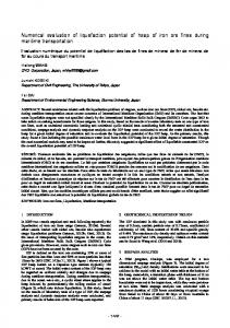
2. Key Features of UBC3D-PLM 2.1. Yield surface Mohr-Coulomb yield function generalized in 3-D principal stress space is used in UBC3DPLM model (Alexandros & Vahid, 2013) as presented in Figure 1.
Fig. 1. Mohr-Coulomb yield surface in principal stress space.
The critical yield surface could be defined as given by Equation (1):
fm
' ' max min ' ' ( max min c' cot p' ) sin mob 2 2
(1)
′ ′ Where, 𝜎𝑚𝑎𝑥 and 𝜎𝑚𝑖𝑛 are the maximum and minimum principal stresses respectively, 𝑐 ′ is the cohesion of the soil, 𝜙𝑝′ is the peak friction angle of the soil and 𝜙𝑚𝑜𝑏 is the mobilised friction angle during hardening.
2.2. Elasto-plastic behaviour The elastic behaviour, which occurs within the yield surface is controlled by two parameters expressed in terms of the elastic bulk modulus 𝐾𝐵𝑒 and the elastic shear modulus 𝐾𝐺𝑒 as shown below:
p' K k PA PA e B
me
p' K k PA PA e G
(2)
e B
ne
(3)
e G
Where, 𝑝′ is the mean effective stress, 𝑃𝐴 is the reference stress (usually equal to 100kPa), 𝑘𝐵𝑒 and 𝑘𝐺𝑒 are the bulk and shear modulus numbers respectively and, me and ne are the elastic exponents which define the rate dependency of stiffness. The hardening rule as reformulated by Tsegaye (2011) in UBC3D-PLM model is given as: 2
p P sin mob d sin mob 1.5KGp A 1 R f d sin P P peak A m np
(4)
Where, 𝑑𝜆 is the plastic strain increment multiplier, 𝑛𝑝 is the plastic shear modulus exponent, 𝜙𝑚𝑜𝑏 is the mobilised friction angle, which is defined by the stress ratio, 𝜙𝑝𝑒𝑎𝑘 is the peak friction angle and 𝑅𝐹 is the failure ratio 𝑛𝑓 /𝑛𝑢𝑙𝑡 , ranging from 0.5 to 1.0.
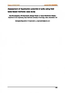
2.3. Cyclic mobility This behaviour is presented in Figure 2 picturing the process of cyclic mobility of dense sand. The stiffness degradation is computed as follows:
K Gp K Gp , primarye E dil
(5)
Edil min(110 * dil , fac post )
(6)
Where 𝜀𝑑𝑖𝑙 is accumulation of the plastic deviatoric strain, which is generated during dilation of the soil element and the input parameter 𝑓𝑎𝑐𝑝𝑜𝑠𝑡 is the value of the exponential multiplier term.
Fig. 2. Undrained cyclic shear stress path reproduced with UBC3D-PLM for dense sand. Cyclic mobility, stiffness degradation and soil densification are referenced on the graph.
2.4. Undrained Behaviour The increment of the pore water pressure is computed by the following equation:
dp w
Kw d v n
(7)
Where, 𝐾𝑤 is the bulk modulus of the water, 𝑛 is the soil porosity and 𝑑𝜀𝑣 is the volumetric strain of the fluid. The bulk modulus of water is dependent upon the degree of saturation of the soil. The bulk modulus of the unsaturated water is defined as follows:
K
unsat w
K wsat K air SK air 1 S K wsat
(8)
Where 𝐾𝑤𝑠𝑎𝑡 is the bulk modulus of the saturated water and 𝐾𝑎𝑖𝑟 is the bulk modulus of air, which equals 1kPa in this implementation having the minimum value that allows avoiding the generation of pore pressures during modelling dry sand 𝑆 is the degree of saturation.
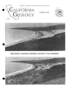
3. Validation of the UBC3D-PLM in Element Test 3.1. Validation of the UBC3D-PLM in Monotonic Loading The validation of the UBC3D-PLM in monotonic loading is presented in this section. The input parameters for modelling the tri-axial compression test (TxC) and the direct simple shear test (DSS) on loose Syncrude sand are given in Table 1. The results of the UBC3DPLM are in a good agreement with the experimental data (Puebla & Byrne & Philips, 1997) as shown in Figure 3.
Fig. 3. Monotonic Loading. (Left: undrained tri-axial compression, right: undrained simple shearing). Table 1. UBC3D input parameters for all the validation tests. Parameter Syncrude S.(TxC, Fraser S. (Cyclic DSS) DSS)
Cargo(FEM)
p
33.7
33.8
31.2
cv
33
33
34.6
k Be
300
607
720
k Ge
300
867
1031
K Gp (TxC )
310
-
K Gp (DSS )
98.3
266
700
me ne
0.5
0.5
0.5
np
0.5
0.4
0.4
Rf
0.95
0.81
0.74
N1(60)
8
8
13
fac hard
1
1
0.45
fac post
0
0.6
0.01
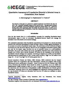
3.2. Validation of the UBC3D-PLM in Cyclic Loading The behaviour of loose Fraser sand under cyclic direct simple shear is modelled and the numerical results are compared with experimental data as published by Sriskandakumar (2004). The relative density (RD) of the tested sand is 40%. In Figures 4, the evolution of
stress-strain is presented. The applied CSR equals 0.08. The vertical applied stress is 100 kPa. The K0 factor is assumed to be 1 for simplification.
(a) Vertical effective stress-shear stress curve
(b) Simulation results and experiment data Fig. 4. Cyclic DSS stress controlled (RD=0.4 CSR=0.08
v =100kpa).
4. Cargo Liquefaction in a Finite Element Scheme 4.1. Evaluating Cargo Liquefaction The soil-water characteristic curve is the basis for estimating the dynamic analysis of particles. Unsaturated particles are composed of three phases; including particle skeleton (solid), pore water (liquid) and pore air (gas). The air-water interface is subjected to surface tension. In the unsaturated particles, the pore air pressure and pore water pressure are unequal with the latter greater than the first. The interface is subjected partly to pore air pressure and partly to larger pore water pressure. The pressure difference (i.e., pore air pressure minus pore water pressure) across the interface of air and water is called the matric suction. Matric suction is generally the key parameter describing the mechanical property of unsaturated particles.
In the capillary tube, the surface between pore air and pore water displays a curved interface. The fluid pressure of the interface with the tube side walls is discontinuous. If the upside of the interface is connected with the atmosphere, the upside pressure interface is larger than the water pressure. The pressure difference is called matric suction. S depends on the curvature of the interface and surface tension.
S ua uw
(9)
The soil-water characteristic curve (SWCCs) relates the water content or degree of saturation to matrix suction of a particle. A representative SWCCs is shown in Fig 5. It can be seen that different iron ore has different water holding ability. With the cargo compaction, the volume decreases resulting in increasing pore water pressure and decreasing matric suction of cargoes. Cargoes cannot hold any water in the case when suction equals zero. Water is progressively displaced in the hold base, which may result in some portions or all of the cargo developing a flow state. For earthquake liquefaction, the acceleration is large and soil could be regarded as undrained soil, where acceleration for cargo liquefaction is small and the water could drain from cargoes. When the degree of saturation is 100% and water comes out from the cargoes, the cargoes may display movement behaviour that characterises liquids. Therefore, suction=0 is taken as the onset of cargo liquefaction.
Fig. 5. Soil-water characteristic curves.
Fig. 6. Centrifuge test model.
4.2. Centrifuge Test The influence of the degree of saturation on the free field response is investigated. The geometry of layer is shown in Figure 6. Locations L, N, O are monitored through the test. The initial degree of saturation is supposed to be uniform. The degree of saturation involves: S=99.0%, 97.0% and 94.0%. The initial stress may have a great influence on the results and the initial stress used is due to the gravity action during all the tests. The boundary conditions are defined as: at the base of layer, the vertical displacement is blocked, and the input energy is sinusoidal horizontal acceleration with 2 amplitude 0.02m / s and frequency 2HZ. At the lateral boundaries, the horizontal displacement is blocked. The model parameters are listed in Table 1.
(a) Degree of saturation=94%
(b) Degree of saturation=97.0%
(c) Degree of saturation =99.0% Fig. 7. Evolution of suction, effective stress and pore water pressure of the column during centrifuge test.
From Figure 7, it can be seen that variation of the degree of saturation has a significant influence on matric suction, effective stress and pore water pressure generation. When the matric suction decreases to 0, the degree of saturation turns 100%. From the figure, after full degree of saturation, the pore water pressure increases rapidly and the effective stress decreases to zero with liquefaction occurring immediately. When the degree of saturation is less than 94%, the onset of liquefaction at point L could be delayed to 23s. With the increase in the initial degree of saturation, the onset of liquefaction becomes easier.
4.3. Shaking Table Test Shaking table tests considering sway motion of a ship with different amplitude, frequency and initial degree of saturation of cargoes are investigated to predict time-domain characteristics during liquefaction based on UBC3D-PLM Model in commercial software PLAXIS. The geometry of layer is shown in Figure 8. Locations M, L, K, P, O and N are monitored through the test. The initial degree of saturation is supposed uniform and varies as 99%, 95.16% and 92.38%. The frequency varies as 0.25HZ, 0.35HZ and 0.5HZ. The amplitude varies as 0.02m, 0.04m and 0.06m. The boundary conditions are defined as: rigid box is used in the shaking table test; at the base of layer, the vertical displacement is blocked, and the input energy is sinusoidal horizontal displacement condition. At the lateral boundaries, the horizontal displacement is free and has the same motion as the base of the box. The initial stress due to gravity is shown in Figure 8.
Fig. 8. Shaking table test model. (Left: monitor points, right: the effective stress contour after gravity action).
From Figure 9 in the calculation of amplitude 0.04m, frequency 0.25HZ and degree of saturation 95.16%, it can be seen that the soil near locations L, O and K is at the limit of liquefaction due to severe contraction. Locations M and P show dilation and N has a high effective stress, hence difficult to liquefy. Emphasis could be put on the middle column of location O. From Figure 9, it can be seen that the higher degree of saturation, frequency and amplitude, the easier the onset of liquefaction. Due to the interaction between soil and rigid box, liquefaction of the soil displays more complicated behaviour from the curves of effective stress. From (a) to (c), variation of the amplitude and frequency have small impact on liquefaction, whilst degree of saturation has just the opposite effect.
a) Evolution of suction during shaking table test
c) Variation with frequency
b) Variation with amplitude
d) Variation with degree of saturation
Fig. 9. Evolution of suction at the middle of the column during shaking table test.
5. CONCLUSIONS Tests for monotonic loading and cyclic loading agree well with experimental data. The Finite Element Method combined with the UBC3D-PLM model could be used to evaluate the potential for cargo liquefaction. Accurate description of cargo properties is the key factor to predict cargo liquefaction. With the higher degree of saturation, frequency and amplitude, cargo is less resistant to liquefaction. Among these three factors, the only one that can be controlled is the degree of saturation. Reducing the degree of saturation of cargoes will enormously reduce the ensuing problems of cargo ships during transportation of granular cargoes. This method in the paper could be potentially used as a reference and possibly support the development of cargo liquefaction assessment based on time domain analysis.
References Beaty, M. and Byrne, P., 1998 An Effective Stress Model for Predicting Liquefaction Behaviour of Sand ASCE Geotechnical Earthquake Engineering and Soil Dynamics (geotechnical special publication III), Vol. 75(1), pp. 766-777. Petalas, Alexandros. and Galavi, Vahid., 2013 Plaxis Liquefaction Model UBC3D-PLM PLAXIS Report. Puebla, H., Byrne, M., and P.Philips, P., 1997 Analysis of canlex liquefaction embankments prototype and centrifuge models Canadian Geotechnical Journal, Vol. 34, pp. 641-651. Sriskandakumar, S., 2004 Cyclic loading response of fraser sand for validation of numerical models simulating centrifuge tests Master's Thesis, University of British Columbia, Department of Civil Engineering. Tsegaye, A., 2011 Plaxis Liquefaction Model PLAXIS Report. G.R. Martin, W.D.L. Finn, and H.B. Seed., 1975 Fundamentals of liquefaction under cyclic loading Journal of the Geotechnical Engineering Division, ASCE, 101.