Numerical Simulation of Flood Wave Propagation in ...

Numerical Simulation of Flood Wave Propagation in Two-Dimensions in Densely Populated Urban Areas due to Dam Break Ismail Haltas, Sebnem Elçi & Gokmen Tayfur

Water Resources Management An International Journal - Published for the European Water Resources Association (EWRA) ISSN 0920-4741 Water Resour Manage DOI 10.1007/s11269-016-1344-4

1 23

Your article is protected by copyright and all rights are held exclusively by Springer Science +Business Media Dordrecht. This e-offprint is for personal use only and shall not be selfarchived in electronic repositories. If you wish to self-archive your article, please use the accepted manuscript version for posting on your own website. You may further deposit the accepted manuscript version in any repository, provided it is only made publicly available 12 months after official publication or later and provided acknowledgement is given to the original source of publication and a link is inserted to the published article on Springer's website. The link must be accompanied by the following text: "The final publication is available at link.springer.com”.

1 23

Author's personal copy Water Resour Manage DOI 10.1007/s11269-016-1344-4

Numerical Simulation of Flood Wave Propagation in Two-Dimensions in Densely Populated Urban Areas due to Dam Break Ismail Haltas 1 & Sebnem Elçi 2 & Gokmen Tayfur 2

Received: 19 November 2015 / Accepted: 2 May 2016 # Springer Science+Business Media Dordrecht 2016

Abstract Dams are important structures having many functions such as water supply, flood control, hydroelectric power and recreation. Although dam break failures are very rare events, dams can fail with little warning and the damage at the downstream of the dam due to the flood wave can be catastrophic. During a dam failure, immense volume of water is mobilized at very high speed in a very short time. The momentum of the flood wave can turn to a very destructive impact force in residential areas. Therefore, from risk point of view, understanding the consequences of a possible dam failure is critically important. This study deals with the methodology utilized for predicting the flood wave occurring after the dam break and analyses the propagation of the flood wave downstream of the dam. The methodology used in this study includes creation of bathymetric, DEM and land use maps; routing of the flood wave along the valley using a 1D model; and two dimensional numerical modeling of the propagation and spreading of flood wave for various dam breaching scenarios in two different urban areas. Such a methodology is a vital tool for decision-making process since it takes into account the spatial heterogeneity of the basin parameters to predict flood wave propagation downstream of the dam. Proposed methodology is applied to two dams; Porsuk Dam located in Eskişehir and Alibey Dam located in Istanbul, Turkey. Both dams are selected based on the fact that they have dense residential areas downstream and such a failure would be disastrous in both cases. Model simulations based on three different dam breaching scenarios showed that maximum flow depth can reach to 5 m at the border of the residential areas both in Eskişehir and in Istanbul with a maximum flow velocity of 5 m/s and flood waves having 0.3 m height reach to the boundary of the residential area within 1 to 2 h. Flooded area in Eskişehir was estimated as 127 km2, whereas in Istanbul this area was 8.4 km2 in total.

* Gokmen Tayfur [email protected]

1

Department Civil Engineering, Zirve University, Gaziantep, Turkey

2

Department Civil Engineering, Izmir Institute of Technology, Urla, Izmir, Turkey

Author's personal copy I. Haltas et al.

Keywords Bathymetry . DEM . Land use maps . Dam break . Flood wave . Numerical modeling . Urban area . Flood maps

1 Introduction In the rare case of a dam failure, especially if it has a large volume of reservoir behind, the magnitude of the downstream flood wave can be so high that it can cause structural and erosional damage. The catastrophe is often sudden and can cause many losses of lives. Vajont Dam, a concrete arch dam with 267 m height in Venice, Italy, collapsed in 1963. It was the most disastrous event in dam failure history with a death toll of more than 2,000 people (Guney et al. 2014). The rock-fill Tous Dam in Spain, as a result of heavy rainfall, broke down in 1982, resulting in flooding of 300 km2 of inhabited land, towns, and villages. Flood depths had reached up to 7 m and 200,000 people were affected, of which 100,000 were already evacuated and the total death toll was 8 (Alcrudo and Mulet 2007). Planning ahead in case of such a disaster would require the prediction of the possible flow velocities, when and where the flood waves can reach at the downstream areas, and creation of an awareness of the possible effects of the failure for the people living downstream of dams. Studies for modeling of the flood wave propagation after the dambreak were conducted in the past, and mostly 1D models (Yanmaz et al. 2001; Macchione 2008; Petaccia and Natale 2008; Froehlich 2008) were utilized. Of these models; HECRAS developed by the Hydrologic Engineering Center of USACE and FLDWAV developed by the U.S. National Weather Service (NWS) (NOAA 2000) have been applied for a variety of rivers and streams. These models describe the unsteady flow in a natural river by one-dimensional shallow water (or Saint-Venant) equations with the assumption of small water surface variation, and hydrostatic pressure distribution. In the kinematic wave solution approach, for which all space and time derivatives are neglected in the momentum equation, the flow depth in the rising and falling stages is the same for the same discharge, and no hysteresis is observed (Altinakar 2008). In reality however, for a given discharge in unsteady flow, the stage discharge curve yields different depths in rising and falling stages. Prediction of the propagation of the flood wave on actual topography is a challenge due to drying/wetting process, discontinuities in the flow and the sudden changes at the bottom slope. Dam break flows may involve discontinuities such as hydraulic jumps and can have mixed flow regimes (sub-, super-, and trans-critical) in the same computational domain. Bozkus and Guner (2001); Bozkus and Bag (2011) applied DAMBRK and FLDWAV models to several dams in Turkey where they modeled the results of dam failure in 1D. 2D models (Brufau et al. 2002; Ying 2005; Singh et al. 2011; Qi and Altinakar 2012; Mahdizadeh et al. 2012) that solve either full dynamic or simplified forms of conservative forms of shallow water equations or coupled models (1D-2D) that solve both 1D river flow and 2D overland flow using full dynamic or simplified forms of conservative forms of shallow water equations are necessary for modeling of the resultant effects of the failure on the downstream residential area. These models should also be capable of simulating the complex flow conditions. Alcrudo and Mulet (2007); Pilotti et al. (2011), and Moramarco et al. (2013) simulated historical dam break flows, predicting inundated areas using data on dam properties, land use, and topography. However, in this study, the focus is on the analysis of propagation of peak flow at the urbanized area, and to point out how the settlements downstream will be affected from a possible dam failure.

Author's personal copy Numerical Simulation of Flood Wave Propagation in Two-Dimensions

Analysis of geospatial data made progress with recent advances in GIS technologies and this increased the use of 2D numerical models for more accurate predictions of flood wave propagation. Among the available 2D models; MIKE FLOOD, developed by DHI Group, Denmark, CCHE2D-DAMBREAK model developed by the National Center for Computational Hydroscience and Engineering (NCCHE) at the University of Mississippi, FLO2D: Two-dimensional Flood Routing model, and TELEMAC-2D developed by the EDF, France may be listed. The CCHE2D-DAMBREAK model is widely used in the USA for execution of military hydrology related studies (Ying 2005). The model solves the conservative form of the two-dimensional shallow water equations over a complex topography defined by a regular mesh. FLO-2D is a dynamicflood routing model that simulates channel flow, unconfined overland flow and street flow over complex topography and roughness. The basic model is freely distributed and it is approved by the US Federal Emergency Management Agency (FEMA) for flood insurance studies. The model uses the full dynamic wave momentum equation and a central finite difference routing scheme with eight potential flow directions to predict the progression of a flood hydrograph over a system of square grid cells (http://www.flo-2d.com/). Aside from the commercial software packages, researchers have developed their own models for their studies. One of such models is LISFLOOD-FP which was developed with joint effort between the University of Bristol and the EU Joint Research Centre based on the original code developed by Bates and de Roo (2000). LISFLOOD-FP is a two-dimensional raster-based inundation model specifically designed to simulate floodplain inundation in a computationally efficient manner over complex topography. Flood Wave Routing (FLOW-R2D) was recently developed by Tsakiris and Bellos (2014), based on 2D Shallow Water Equations. The model has the ability to capture the most important topographic peculiarities. FLOW-R2D has the ability to describe discontinuities of the flow and can incorporate the GIS data for estimating the dominant model parameters. In this study, HEC-RAS is applied for modeling of dam break flood hydrograph for various dam breaching scenarios and FLO-2D is utilized for the numerical modeling of the propagation of flood wave downstream of the dam. Dambreak flood hydrographs for various dambreak scenarios are routed along the valley downstream of the dam, on the floodplains and through the densely populated urban areas in two different sites inIstanbul and Eskisehir province of Turkey.

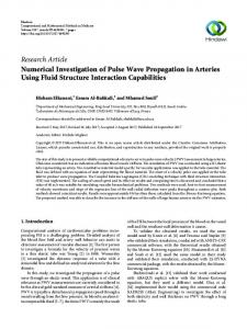
2 Study Sites Istanbul is a rapidly developing city and as it is the case for all developing cities, settlement areas extend at a fast pace (population as of 2014 ~ 14 million). When Alibey Dam (see Fig. 1) was constructed in between 1975 and 1983, for the purpose of supplying drinking water to the city, the downstream area was a rural area. Currently however, the area is completely occupied by the residential settlements. The dam is an embankment dam, 30 m high, having a volume of 2 hm3earth fill. The reservoir volume is 67 hm3 and the surface area is 5 km2 at the normal water level. The failure of the dam would result in an extensive damage and deaths that is why this dam was selected as one of the study sites.


Fig. 1 Maps of Alibey Dam in Istanbul and Porsuk Dam in Eskisehir, Turkey (Source: GoogleEarth)

Porsuk Dam is a concrete gravity dam (see Fig. 1) and was built in between 1966 and 1972 to supply drinking water to the city of Eskişehir, located 20 km downstream of the dam (population as of 2014 ~ 800, 000) and for irrigation and flood control purposes. The dam is 50 m high, having a volume of 223 dm3; the reservoir volume is 525 hm3 and the surface area is 27.7 km2 at the normal water level. Considering its size, the selected dam also constitutes a threat to the areas, including the city of Eskisehir, downstream of it.

3 Methodology The methodology used in this study includes creation of maps (bathymetric, DEM and land use maps); modeling of dam break flood hydrograph for various dam break scenarios using a 1D model (HEC-RAS); and numerical modeling of the propagation of flood wave at the downstream of the dam on the plains and in the urban areas using a two dimensional model (FLO-2D). The 1D model is employed only to model the dambreak hydrograph. The 2D model performs the routing of the flood hydrographs in the valley and in the floodplain. Therefore, the flood hydrograph calculated by the 1D model just at the downstream cross section of the dam is used as the upstream boundary for the 2D model. Although the flood hazard in the valley is not mapped based on the 1D model results, for the stability of the 1D model and accuracy of the flood hydrograph at the downstream of the dam, 1D model is extended along the valley. In this approach extremely large flood discharges from dambreak compensates the inadequacy due to modeling a valley with relatively steep topography using 2D model at a medium grid resolution. It is also possible to model the flood routing along the valley using the 1D model and in the floodplain using the 2D model as applied in Haltas et al. (2016) especially for the Porsuk Dam site, yet that would result in inhomogeneous model results between the valley and the floodplain and not preferred in this study.


3.1 Creation of Data in GIS Since 1970s, Geographical Information Systems (GIS) have been widely used as a powerful tool for the collection, storage, retrieval, analysis and presentation of geographically referenced information. GIS has a wide range of applications in water resources and provides solutions through integration with the hydraulic models. Among the application areas of GIS for water resources management; classification of soil type and vegetation, definition of land use, determination of watershed boundaries, selection of dam site, prediction of reservoir capacity, prediction of erosion and deposition and modeling of groundwater flow can be listed. The advances in GIS technology enabled numerical modeling of basin parameters considering their spatial heterogeneity, which decreased the uncertainty in the model and led to more reliable simulation results. In this study, GIS is used primarily for the creation of reservoir bathymetry data, digital elevation and land use maps for the downstream area of the dams. Details of the creation of maps are given in the application section.

3.2 Hydraulic Modeling of Dam Break via HEC-RAS Hydraulic modeling of dam break via HEC-RAS includes three steps: (1) Routing the inflow through the reservoir, (2) estimating dam breach characteristics, and (3) downstream routing. In HEC-RAS, routing of the flood in the reservoir can be achieved either by the unsteady flow routing or by the level pool routing. Since only reservoir volume upstream of the dam is considered in this study, level pool routing is assumed to be sufficient to model the dam break. To model the reservoir using level pool routing, the dam is modeled as an inline structure. The storage area is defined and connected to a downstream reach. Then, the river reach is defined such that it has two cross sections inside the pool. One of these cross sections is tied to the storage area so that it has water surface elevation during the simulations and the other constitutes the boundary condition for the inlet structure. Elevation-volume curve is also provided as input to the model and the minimum elevation of the two upstream cross sections is forced to be equal to the minimum elevation of the storage to avoid instability of the model in the simulations. Second step involved estimating the breach characteristics. The driving forces to failure might be various, including flood event, piping, foundation failure, landslide, earthquake and sabotage. Failure of earth dams occurred mainly due to overtopping (35 %), piping (38 %), and foundation defects (21 %) as reported in the literature (Costa 1985). Definition of breach characteristics is important for the calculation of outflow hydrograph correctly. However it has great uncertainty since we are modeling a possible failure but not the actual case. Of the failure mechanisms (overtopping or piping) characteristics, location and shape of the breach are important. The third step involves modeling of the downstream routing. For an accurate modeling of flood propagation downstream in HEC-RAS, several issues must be considered. Of these, cross section spacing, computational time step, manning roughness and downstream boundary conditions should be carefully defined. Sufficient number of cross sections is required to describe contractions and expansions, changes in bed slope, roughness and discharge. For the maximum spacing, Eq. (1) proposed by Samuels (1989) can be used as a reference. Δx ¼

0:15D S

ð1Þ


where, D is the mean channel depth and S is the slope, and a minimum spacing of 50 ft (15 m) is defined by USACE (2012) for dam break studies to avoid use of smaller time steps at those cross sections. Computational time step can be chosen to satisfy the Courant condition (Eq. 2) since too large time steps would cause numerical diffusion and possible numerical instability and too small time steps would yield too long computational time. Δt ¼

Δx Vw

ð2Þ

where Δt is the time step, Δx is the distance space and Vw is the flood wave speed. For practical applications, maximum average velocity provided by the model can be multiplied by 1.5 to obtain the flood wave speed (USACE 2012). Initial conditions must be set in all cross sections before the simulation starts. So, the user enters initial flows or stages at the cross sections. If low flow is defined, when the unsteady simulations start, the program calculates a much higher flow coming from the reservoir resulting in the instability just below the dam. Initial storage area elevations are also important, since they might also cause instability at the initial start of the simulations. If the storage elevation is set too higher or too lower than the river elevation it is tied to, large discharge either goes to the river or from the river to the storage causing instability. The 1D model requires an initial flow (pilot flow) to run before the dambreak flood arrives to the cross sections. The value of the initial flow is not so important yet it should be large enough to satisfy the numerical stability in the calculations. On the other hand, it should be negligibly small compared to the actual discharge so that it does not affect the results. In this study, for Porsuk Dam, 15 m3/s is used as initial discharge. As the initial elevation of the Porsuk Dam Reservoir, 890.25 meter is assigned which is the maximum operational level of the dam. Similarly, in the Alibey Dam, 52 m3/s is used as initial discharge. As the initial elevation of the Alibey Dam Reservoir, 30 meter is assigned which is the maximum operational level of the dam. Downstream boundary condition is also a source of uncertainty since it is initially unknown. Generally normal depth (Manning equation) or rating curve computed from steady flow simulation is used as downstream boundary condition. In this study normal depth boundary condition is defined at the downstream of the 1D model. The friction slope is set to the average channel bottom slope calculated from the topography.

3.3 Modeling of the Propagation of Flood Wave on the Plains and in the Residential Areas Once the dambreak hydrograph is calculated just at the downstream of the dam, the routing of the flood in the valley and the two-dimensional spreading of the flood wave over the plains is modeled using FLO-2D. FLO-2D is an integrated river and floodplain 2D flood routing model that routes flood hydrographs and rainfall-runoff with many urban detail features specified by the area and width reduction factors and surface roughness values. Using the finite difference method for each grid cells, FLO-2D model solves full dynamic wave and volume conservation equations. Thus, two-dimensional spread of flood wave is calculated on grid cell systems. From the computational results of the two dimensional model it is possible to obtain the following flood characteristics in each grid cell in the computation domain; (1) Inundation extend, (2) Maximum flow depth, (3) Maximum water elevation, (4) Maximum flow velocity,


and (5) Time to reach to maximum flow depth. The ArcGIS software is used to develop the flood hazard maps in GIS environment. FLO-2D model performs the hydrodynamic calculations for grid cells within a computational domain. The 2D domain boundary should be defined such that flood wave can freely propagate and limited only by the topographic features. Defining an excessively large computational domain, on the other hand, results in large number of grid cells and therefore results in longer computational hours. An optimal model boundary is determined by the trial and error procedure. The outflow cells are selected far away from the residential area, so that the downstream boundary condition does not affect the flood characteristics in the residential area. Normal depth boundary condition is used for the downstream boundaries. The numerical model uses a friction slope same as the bottom slope automatically calculated from the topography at the outflow cells. For selection of the optimum grid cell size, the criterion given in the FLO-2D User Guide (2009a) is followed: 0:3 m3 =s=m2 ≤Qmax =Agrid ≤3 m3 =s=m2

ð3Þ

where, Qmax is the maximum discharge in a grid cell, Agrid is the area of the grid cell. For the Porsuk Site a grid cell size of 100 m is defined and the total number of grid cells in the computational domain is 35,365. 11-hour long simulation took 72.02 CPU hours at Intel Core i5 @3.26 Hz processor. For the Alibey Site a grid cell size of 50 m is defined and the total number of grid cells in the computational domain is 26,350. 5-hour long simulation took 21.0 CPU hours at Intel Core i5 @3.26 Hz processor. The effect of the buildings on storage and conveyance characteristics at grid cells is among the most important factors in urban flood modeling. Especially in course grid modeling where the grid cell size is a lot bigger than the overall building footprints, buildings can only be modeled as subgrid heterogeneity. One of the most common approaches for modeling the effect of the buildings on storage and conveyance is using storage reduction and conveyance reduction factors at each grid cells. Chen et al. (2012a) abstracted the building features in coarse grids using the building coverage ratio (BCR) and the conveyance reduction factor (CRF) parameters in a 2D model to simulate flooding in urban areas. They compared their BCR and CRF improved coarse grid model (at 20 m resolution) with a finer grid model (at 4 m resolution) with buildings burned in to the DEM. The outcome of comparison showed the proposed model can provide a much better accuracy of modeling results at a marginally increased computing cost. In another study, Chen et al. (2012b) adopted multiple layers in flood modeling to reflect individual flow paths separated by buildings within a coarse grid cell. In their approach, the cell in each layer has its own parameters (elevation, roughness, building coverage ratio, and conveyance reduction factors) to describe itself and the conditions at boundaries with neighborhood cells. The multi layer approach basically addresses the shortcoming of the single layer storage and conveyance reduction model (Chen et al. 2012a). They have tested the multilayer cell approach on both the synthetic case study and the real world urban area. The test results show that the proposed multi-layered approach further improves the accuracy of the model at grid cells around the buildings by including the flow path separations within the coarse grid cell in the model with an insignificant additional computing cost. Bellos and Tsakiris (2015) have tested reflection boundary, the elevation rise and the roughness increase methods for building


representation in the flood-prone built–up areas. According to the model performance and the computational cost, the reflection boundary method is claimed to be the most efficient way for representing buildings of the urban environment. Yet the reflection boundary method requires fine grid resolution and may not applicable in the case of lack of high-resolution topographic data or limited computational resources. In such cases, they recommend roughness increase method as a more suitable approach. Schubert and Sanders (2012) investigated four different building treatment methods -namely building resistance (BR), building block (BB), building hole (BH) and building porosity (BP)- for urban flood inundation models with irregular mesh. Dottori and Todini (2013) tested a simplified 2D diffusive wave model in an urban flood experiment. They tested a simplified porosity-based approach and the increase of roughness for urban grid cells. Their results show that tested methods for representing the urban district provided similar results to detailed grid representations, suggesting that they could be proficiently used in combination with reduced complexity models. The pre-processing unit of FLO-2D software Grid Developer System (GDS) allows to representation of buildings and other obstructions by using two parameters namely Area Reduction Factor (ARF) and Width Reduction Factor (WRF). ARF and WRF parameters work similar to the BCR and CRF parameters introduced in Chen et al. (2012a). The ARF parameter can take a value between 0 and 1, where ARF = 1 means that the grid cell is totally blocked. Similarly the WRF parameter in any direction can take value between 0 and 1, where WRF = 1 means that the conveyance in the given direction is totally blocked. Unlike the 2D hydrodynamic model employed in Chen et al. (2012a), FLO-2D model calculates conveyance both in the direction of neighbor and diagonal cells. That

Fig. 2 Bathymetry maps for Alibey and Porsuk Dam Reservoirs


Fig. 3 Digital elevation models of Alibey and Porsuk Dams’ downstream areas

makes the assignment of WRF in each cell more complicated. Although the GDS preprocessing module of FLO-2D does support automated assignment of ARF

Fig. 4 Roughness maps of Alibey Dam and Porsuk Dam downstream areas

Author's personal copy Alibey

45 40 35 30 25 20 15 10 5 0

Porsuk

900 Elevation (m)

Elevation (m)

I. Haltas et al.

890 880 870 860 850

0

20 40 60 80 100 120 Volume (10E3 m3)

840 0

100 200 300 400 500 600 Volume (10E6 m3)

Fig. 5 Elevation-volume curves of Alibey and Porsuk reservoirs

parameters it does not support fully automated assignment of WRF. Considering the area and urban density of the study sites, manual assignment of WRF parameters is very cumbersome task and not performed in this study. On the other hand ARF parameters are assigned to grid cells. A spatially variable Manning friction factor is assigned to grid cells by considering vegetation and land use characteristics determined from maps created by GIS. The roughness complexities in the urban areas due to the building structures are modeled using the ARF parameters. It is difficult to estimate the resistance to flood wave due to the cars and other relatively small objects in the floodplain. Most probably they are going to be mobile during the propagation of such a big flood wave. The assigned Manning n value in the 2D model is adopted from the reference Manning n values provided in the FLO-2D Reference Manual (2009b).

Table 1 Dam Breaching Scenarios used for Alibey and Porsuk Dams Alibey Dam Parameters

Scenarios Best case

Average case

Worst case

Breaching Mode

Piping

Overtopping

Piping

Breaching Completion Duration (hr)

2

1

0.25

Final Breaching Bottom Width (m)

40

80

150

Peak Flood Discharge (m3/s)

8,603

14,471

28,194

Total Inundation Area (km2)

7.95

8.38

8.45

Maximum Flow Depth (m)

13.83

15.54

16.01

Porsuk Dam Parameters

Scenarios Best case

Average case

Worst case

Breaching Mode

Piping

Overtopping

Piping

Breaching Completion Duration (hr)

1.1

0.7

0.3

Final Breaching Bottom Width (m) Peak Flood Discharge (m3/s)

20 66,374

60 100,874

120 200,880

Total Inundation Area (km2)

123.26

126.94

131.13

Maximum Flow Depth (m)

30.17

34.78

42.45


4 Prediction of Flood Wave Propagation 4.1 Creation of Data in GIS Hydrographic maps of the reservoirs (4 for Alibey Reservoir and 9 for Porsuk Reservoir) are obtained from State Hydraulic Works of Turkey. First step is to specify coordinate system for these printed maps. To specify the coordinate system, define projection tool within ArcToolBox projection is used and projection is defined as UTM-WGS 1984-Northern Hemisphere and zone is selected as 35 N.prj. Then, the coordinates of all 4 corners of the

Fig. 6 Cross sections used in modeling of 1D flow of flood propagation via HEC-RAS along the Alibey and Porsuk creeks after the Dam-break


Routed Hydrograph for Porsuk 200000

25000

Best Case

20000

Worst Case

Average Case

Best Case Average Case Worst Case

150000 Q (m3/s)

Q (m3/s)

Routed Hydrograph for Alibey 30000

15000 10000

100000 50000

5000 0 0

1

2

3 4 5 time (hr)

6

7

0 0

5

10 time (hr)

Fig. 7 Routed hydrographs via HEC-RAS for Alibey and Porsuk Dam break scenarios

Fig. 8 Maximum flow depth observed after the failure of Alibey Dam

15

20


hydrographic maps are input using add control point tool located in the GeoReferencingtool. The maps are then rectified and saved as projected maps. For digitizing of these maps, a new file GeoDatabaseis constructed and layers to represent bathymetry data and reservoir are defined via new-feature class tool. Create feature tool is used for digitizing and line type is selected for bathymetry, and polygon type is selected for the reservoir representing feature class. Once digitizing is completed, bathymetry curves are transformed to TIN and then to raster to obtain bathymetric maps. Figure 2 shows the bathymetry maps obtained for Alibey and Porsuk Dam Reservoirs. Following the creation of the bathymetric maps, digital elevation models (DEM) for the downstream area of the dams are created from 1:25000 scale standard topographical maps provided by the General Command of Mapping in Turkey. Since these maps are provided in digital format, they are first merged and transformed to TIN then to raster to obtain DEM maps (Fig. 3). Next step is the creation of roughness maps of the study areas to be used in the numerical models. For this purpose, first Google Earth images of the study sites are merged and saved as

Fig. 9 Maximum flow depth observed after the failure of Porsuk Dam


picture, then coordinate systems are specified and roads, forests, buildings, rivers and reservoirs are digitized via editor tool as new layers. Figure 4 shows the roughness maps for the downstream areas of the dams.

4.2 Modeling of Dam Break via HEC-RAS Hydraulic modeling of dam break via HEC-RAS is achieved by following the three steps: (1) Routing the inflow through the reservoir, (2) estimating dam breach characteristics, and (3) downstream routing. Since reservoir volume of the dam alone is considered in this study, level pool routing is utilized for inflow routing. Figure 5 shows the elevation volume curves used in Alibey and Porsuk dambreak simulations. These curves are obtained from the topographical maps produced before the filling of the reservoirs. During a piping failure breach, orifice pressure flow equation is applied to calculate the flow rate of water flowing through the dam. Recommended value of 0.5 (USACE 2014) is used as piping coefficient in the study. Table 1 presents the breaching parameters utilized for the simulation of Alibey Dam and Porsuk Dam failures. In Table 1, breaching mode, breaching completion duration, and final breach bottom width were the parameters required to be defined in HEC-RAS for the modeling of the breaching process. The other values in Table 1 i.e. peak flood discharge, total inundation area, and maximum flow depth are the calculated values by the 1D and 2D model based on the first given set of parameters.

Fig. 10 Maximum flow velocities observed after the failure of Alibey Dam


HEC-GeoRAS for ArcMapis an extension tool designed to process geospatial data for applications in HEC-RAS. The cross sections along the creeks downstream of the dams are modeled using this extension, which allows users to create a HEC-RAS import file containing geometric attribute data from an existing DEM. Construct XS CutLines tool is used to create five cross sections, each 50 m apart at the downstream of Alibey Dam (Fig. 6). The elevations for the cross sections are derived from the DEM data via InterpolateLine tool. Graphical presentation of the cross section profiles is obtained by utilizing Point Profileand Profile Graph tools. For the creek located downstream of the Porsuk dam however 67 cross sections, each 100 m apart, are used to model the flood routing along the valley (see Fig. 6). The routed hydrographs simulated by HEC-RAS are given in Fig. 7 for Alibey and Porsuk Dams. These routed hydrographs after the dam break are set as upstream boundary conditions for the two dimensional numerical model used for the propagation of flood wave on the plains. The dambreak flood hydrograph calculated by HEC-RAS was distributed over two adjacent grid cells for the Porsuk Dam and over four grid cells for the Alibey Dam along the cross section just at the downstream of the dams as the upstream boundary condition for the two-dimensional model.

4.3 Modeling of the Propagation of Flood Wave on the Plains The flood hydrographs (see Fig. 7) from the one-dimensional model are used as the inflow hydrograph in the two-dimensional model. A spatially variable Manning friction factor is

Fig. 11 Maximum flow velocities observed after the failure of Porsuk Dam


assigned to grid cells by considering vegetation and land use characteristics. Manning values of 0.02 for residential areas and of 0.04 for non-residential areas are assigned. Area reduction factor are assigned to grid cells in order to account the reduction in storage capacity of the grid cells occupied fully or partially by buildings. Spatially variable ARF values are assigned to grid cells by using the aerial imagery of the study area. By considering the full flood propagation duration in the preliminary runs, simulation periods for the models are determined. The simulation durations are specified as 11 h for Porsuk Dam Break Case and 5 h for Alibey Dam Break Case. Within the given periods, the peaks of the flood hydrographs are observed to reach the model boundaries. The water depth, flow rate, and flow velocity at each grid point with respect to time are simulated and the results are converted into GIS shapefile format for visual display by the postprocessor of FLO-2D, called Mapper. Maximum flow depths, maximum flow velocities and times to reach maximum flow depths are plotted for both dams based on the overtopping scenario which will be named as average scenario within the text due to the fact that it provided the average peak hydrograph value (see Fig. 7). The average scenario for Alibey Dam has completion time of 1 h and final breach bottom width of 80 m (Table 1). The resulting peak flood hydrograph for this case is calculated as 14,471 m3/s. The average scenario for Porsuk Dam has a completion time of 0.7 h and final breach bottom width of 60 m (Table 1). The resulting peak flood hydrograph for this case is calculated as 100,874 m3/s.

Fig. 12 Time to reach maximum flow depth in residential areas after the failure of Alibey Dam


Maximum flow depths are presented in Figs. 8 and 9 and maximum flow velocities are plotted in Figs. 10 and 11 for Alibey and Porsuk dambreak scenarios, respectively. For downstream of Alibey Dam, maximum flow depth reaches approximately 5 m with a maximum flow velocity of 5 m/s at the residential areas. Flooded area covers 8.4 km2 in total (see Figs. 8 and 10). According to the dambreak scenarios used in the model, maximum flow depth reaches approximately 5 m at the southwest border of the residential area in Eskişehir (approximately 20 km from the dam) with a maximum flow velocity of 5 m/s. At the city center, maximum flow depth exceeds 5 m, with a maximum flow velocity higher than 5 m/s. Flooded area covers 127 km2 in total (see Figs. 9 and 11). Figures 12 and 13 present the arrival time of maximum flow depth for Alibey and Porsuk dam break cases, respectively. Flood waves having 0.3 m height reach to the boundary of the residential area in less than 2 h in the case of Alibey dambreak (see Fig. 12). Flood waves having maximum flow depth reach to the boundary of the residential area in approximately 2 h for the case of Porsuk dambreak. Flood waves reach to the Eskişehir Airport within 2.75 h (see Fig. 13).

Fig. 13 Time to reach maximum flow depth in residential areas after the failure of Porsuk Dam


Fig. 14 Comparison of maximum flow depths observed after the failure of Alibey Dam for different scenarios

5 Sensitivity Analysis Following the simulation of the average scenario cases presented in the previous section, the sensitivity on the maximum flow depth, maximum flow velocity and time to reach maximum flow depth are investigated for the corresponding flood hydrographs resulting from different dam breaching modes. Three different breaching modes in total are used in the analysis for each dam; two piping and one overtopping breaching modes, where the details of these modes are presented in Table 1. For Alibey Dam, breach completion times are selected as 2 and 0.25 h and final breach bottom widths are selected as 40 and 150 m for the best and worst cases respectively. The resulting peak flood hydrographs for the best and worst cases in piping breaching modes are calculated as 8,603 and 28,194 m3/s respectively. For Porsuk Dam, breach completion times are selected as 1.1 and 0.3 h and final breach bottom widths are selected as 20 and 120 m for the best and worst cases respectively. The resulting peak flood

Fig. 15 Comparison of maximum flow depths observed after the failure of Porsuk Dam for different scenarios


Fig. 16 Comparison of maximum flow velocities observed after the failure of Alibey Dam for different scenarios

hydrographs for the best and worst cases in piping breaching modes are calculated as 66,374 and 200,880 m3/s respectively. When maximum flow depths simulated for the downstream part of Alibey Dam resulting from the three different breaching modes are compared, the difference for the worst and average cases was less (3 % of maximum flow depth), whereas this difference increased to 11 % for the best and average scenarios (Fig. 14). When the total inundation areas were compared, it was observed that the flooded areas were almost the same (less than 1 %) for the worst and average cases whereas this difference increased to 5 % for the best and average scenarios. When maximum flow depths simulated for the downstream part of Porsuk Dam resulting from the three different breaching modes are compared, the difference for the worst and average cases was also less (13 % of maximum flow depth), whereas this difference increased to 22 % for the best and average scenarios (Fig. 15). When the total inundation areas

Fig. 17 Comparison of maximum flow velocities observed after the failure of Porsuk Dam for different scenarios


Fig. 18 Comparison of times to reach maximum flow depths observed after the failure of Alibey Dam for different scenarios

were compared, it was observed that the flooded areas were almost the same (less than 3 %) for all the cases in the case of Porsuk Dam failure. When maximum flow velocities simulated for the downstream part of Alibey Dam resulting from the three different breaching modes are compared, the difference for the worst and average cases was about 5 m/s (25 % of maximum flow velocity), whereas this difference reduced to half for the best and average scenarios (Fig. 16). Also, it was observed that, the differences were higher right after the dam and further downstream the differences approached to zero. When the maximum flow velocities were compared for Porsuk Dam, the difference for the worst and average cases and for the best and average cases were about the same (5 m/s corresponding to 25 % of maximum flow velocity), (Fig. 17) and the differences were higher right after the dam and further downstream the differences approached to 0 as it was for Alibey Dam.

Fig. 19 Comparison of times to reach maximum flow depths observed after the failure of Porsuk Dam for different scenarios


When times to reach maximum flow depths in residential areas simulated for the downstream part of Alibey Dam resulting from the three different breaching modes are compared, the difference for the worst and average cases was about 1 h, whereas this difference reduced to half for the best and average scenarios (Fig. 18). Also, it was observed that, the differences were less right after the dam for the best-average comparison whereas for the worst vs. average comparison a more uniform lag was observed throughout the modeling section. When times to reach maximum flow depths in residential areas were compared for Porsuk Dam, the difference for the worst and average cases and for the best and average cases were about the same (0.5 h) for the immediate downstream parts of the dam, (Fig. 19) and the differences increased to 1 h at the residential areas.

6 Conclusions Maximum flow depths, flow velocities and times to reach the maximum depths are simulated and presented for the downstream areas of Alibey and Porsuk Dams, in the case of dam failure occurs. A three step approach is followed for this purpose which involved the creation of maps (bathymetric, DEM and land use maps); modeling of dam break flood hydrographusing the 1DHEC-RAS model and numerical modeling of the propagation of flood wave in downstream area using FLO-2D model. Results based on the average scenarios (based on overtopping breaching mode) indicated that maximum flow depth reaches approximately 5 m at the south-west border of the residential area in Eskişehir with a maximum flow velocity of 5 m/s. At the city center, maximum flow depth exceeds 5 m; with a maximum flow velocity higher than 5 m/s. Flooded area covers 127 km2 in total. Flood waves having 0.3 m height reach to the boundary of the residential area in 2 h. Flood waves reach to the Eskişehir airport after 2.75 h. For downstream of Alibey Dam maximum flow depth reaches approximately 5 m with a maximum flow velocity of 5 m/s at the residential areas. Flood waves having 0.3 m height reach to the boundary of the residential area in less than 2 h. Flooded area covers 8.4 km2 in total. Sensitivity analysis wasperformed to analyze the effects of various breaching modes on the resulting flood hydrograph and thus on the selected simulated parameters. The sensitivity analysis showed that having high (worst case) flood hydrograph peaks have effect on the simulated maximum flow depths. This is more pronounced in the case of best case; when a lower hydrograph peak was simulated (best case) flow depths decreased for 13 % for Alibey and 22 % for Porsuk Dams. The difference observed on total inundation areas for both dams in all cases were less than 5 %. Using different flood hydrographs had significant effects (up to 25 % of maximum flow velocity) on the maximum flow velocities and it was observed that the differences were especially high right after the dam and further downstream the differences approached to zerofor both dams. When times to reach maximum flow depths in residential areas simulated for the downstream parts of the dams, it was observed that the differences increased to 1 h at the residential areas whereas for the areas closer to the dams this lag was about half an hour. Modeling the complexities due to the buildings, roads and other manmade structures in a densely populated urban area may require finer resolution in the hydrodynamic model in order to reduce the subgrid heterogeneity. On the other hand, finer resolution can be obtained in an


expense of higher computational resources for such large flood discharges and floodplain areas. In this study, the effect of the buildings on the flood wave propagation and floodplain inundation is modeled accurately on overall sense using the ARF parameters, yet the subgrid heterogeneity may still cause inaccuracy within the grid cells. Acknowledgments This study was funded by research grant from the Turkish Science Foundation (TÜBITAK) through Project No: 110 M240. We thank TÜBİTAK for this support. We thank BülentKocaman at Turgut Özal University, Civil Engineering Department for producing some of the flood maps.

References Alcrudo F, Mulet J (2007) Description of the Tous Dam break case study (Spain). J Hydraulic Res 45:45–58 Altinakar (2008) Report by working group on dam issues related to floodplain management submitted to association of state flood plain managers Bates PD, de Roo APJ (2000) A simple raster-based model for flood inundation simulation. J Hydrol 236(1):54– 77 Bellos V, Tsakiris G (2015) Comparing various methods of building representation for 2D flood modelling in built-up areas. Water Resour Manag 29(2):379–397 Bozkus Z, Bag F D2011] Virtual failure analysis of Çınarcık Dam. TeknikDergi 22D4]:5675–5688 Din Turkish] Bozkus Z, Guner AI (2001) Pre-event dam failure analyses for emergence management. Turkish J Eng Environ 25:627–641 Brufau P, Vazquez-Cendon ME, Garcia-Navarro P (2002) A numerical model forflooding and drying of irregular domains. Int J Numerical Methods Fluids 39:247–75 Chen SA, Evans B, Djordjevic S, Savic DA (2012a) A coarse-grid approach to representing building blockage effects in 2D urban flood modeling. J Hydrol 426–427:1–16 Chen SA, Evans B, Djordjevic S, Savic DA (2012b) Multi-layered coarse grid modelling in 2D urban flood simulations. J Hydrol 470–471:111 Costa JE (1985) Floods from dam failures. U.S. Geological Survey, Open-File Rep. No. 85–560, Denver, 54 Dottori F, Todini E (2013) Testing a simple 2D hydraulic model in an urban flood experiment. Hydrol Process 27(9):1301–1320 FLO-2D Software Inc (2009) FLO-2D users manual. Documentation. Retrieved from http://www.flo-2d.com/ FLO-2D Software Inc (2009) FLO-2D reference manual. Documentation. Retrieved from http://www.flo-2d.com/ Froehlich DC (2008) Embankment dam breach parameters and their uncertainties. J Hydraulic Eng 134(12): 1708–1721 Guney MS, Tayfur G, Bombar G, Elci S (2014) Distorted physical model to study sudden partial Dam break flows in an Urban area. J Hydraulic Eng 140:11 Haltas I, Tayfur G, Elci S (2016) Two-dimensional numerical modeling of flood wave propagation in an Urban area due to Ürkmez Dam-Break, İzmir, Turkey. Nat Hazards 81:2103–2119 Macchione F (2008) Model for predicting floods due to earthen dam breaching. I. Formulation and evaluation. J Hydraulic Eng 134(12):1688–1696 Mahdizadeh H, Stansby PK, Rogers BD (2012) Flood wave modeling based on a two-dimensional modified wave propagation algorithm coupled to a full-pipe network solver. J Hydraul Eng 138(3):247–259 Moramarco T, Barbetta S, Pandolfo C, Tarpanelli A, Berni N, Morbidelli R (2013) The spillway collapse of the Montedogliodamon the Tiber River (central Italy): data collection and event analysis. J Hydrologic Eng NOAA (2000) National weather service’s FLDWAV computer program Petaccia G, Natale L (2008) Simulation of the Sella Zerbino Catasrophic Dam Break. In Altinakar K, Aydın Ç, Kırkgöz (Eds) Riverflow 2008, 1, 601–607, Kubaba Pilotti M, Maranzoni A, Tomirotti M, Valerio G (2011) 1923 Gleno Dam break: case study and numerical modeling. J Hydraulic Eng 137(4):480–492 Qi H, Altinakar M (2012) GIS-based decision support system for Dam break flood management under uncertainty with two-dimensional numerical simulations. J Water Resour Plann Manage 138(4): 334–341 Samuels PG (1989) Backwater lengths in rivers. Proc Inst Civil Eng, Part 2, Res Theory 87:571–582

Author's personal copy Numerical Simulation of Flood Wave Propagation in Two-Dimensions Schubert EJ, Sanders FB (2012) Building treatments for urban flood inundation models and implications for predictive skill and modelling efficiency. Adv Water Resour 41:49–64 Singh J, Altinakar MS, Ding Y (2011) Two-dimensional numerical modeling of dam-break flows over natural terrainusing a central explicit scheme. Adv Water Resour 34:1366–1375 Tsakiris G, Bellos V (2014) A numerical model for two-dimensional flood routing in complex terrains. Water Resour Manag 28:1277–1291. doi:10.1007/s11269-014-0540-3 USACE HEC-RAS (2012) Documentation. Retrieved from http://www.hec.usace.army.mil/software/hec-ras/ USACE (2014) Using HEC-RAS for dam-break studies. Report No: TD-39, USACE Yanmaz AM, Seçkiner G, Ozaydın V (2001) A method for optimum layout design of concrete gravity Dams. Water Eng Res, Int J Korea Water Resources Assoc 2(4):199–207 Ying X (2005) CCHE2D-DAMBREAK model version 1.0, user’s guide, NCCHE, the University of Mississippi