The variables representing the concentrations of H2, O2, H2O, and. H are explicitly kept ..... stoichiometric coefficient of species i in reaction j and Rj the.
A lumped model for H2/O2 oxidation in the oscillatory regime Genyuan Li and Herschel Rabitz Citation: The Journal of Chemical Physics 102, 7006 (1995); doi: 10.1063/1.469094 View online: http://dx.doi.org/10.1063/1.469094 View Table of Contents: http://scitation.aip.org/content/aip/journal/jcp/102/18?ver=pdfcov Published by the AIP Publishing Articles you may be interested in Reliable anisotropic dipole properties, and dispersion energy coefficients, for O2 evaluated using constrained dipole oscillator strength techniques J. Chem. Phys. 105, 4927 (1996); 10.1063/1.472344 A special singular perturbation method for kinetic model reduction: With application to an H2/O2 oxidation model J. Chem. Phys. 105, 4065 (1996); 10.1063/1.472279 Collisional vibrational energy transfer of OH (A 2Σ+, v′=1) J. Chem. Phys. 104, 6507 (1996); 10.1063/1.471371 Fitting and scaling laws for high temperature Q branch collapse in the O2 stimulated Raman spectra in O2–H2O mixtures J. Chem. Phys. 104, 5347 (1996); 10.1063/1.471650 Accurate quantum probabilities and threshold behavior of the H+O2 combustion reaction J. Chem. Phys. 99, 9310 (1993); 10.1063/1.465548
This article is copyrighted as indicated in the article. Reuse of AIP content is subject to the terms at: http://scitation.aip.org/termsconditions. Downloaded to IP: 128.112.122.110 On: Thu, 18 Dec 2014 19:03:15
A lumped model for H2/O2 oxidation in the oscillatory regime Genyuan Li and Herschel Rabitza) Department of Chemistry, Princeton University, Princeton, New Jersey 08540
~Received 26 October 1994; accepted 3 February 1995! A lumped model for H2/O2 oxidation in the oscillatory regime is constructed by using the approach of approximate constrained nonlinear lumping based on an algebraic method within nonlinear perturbation theory. The fast variables approach zero rapidly such that the lumped model is constructed within a slow manifold by setting the identified fast variables to zero. The model dimension is reduced from 7 to 4. The variables representing the concentrations of H2 , O2 , H2O, and H are explicitly kept unlumped. The lumped model accurately reproduces the main features of the original system, such as oscillatory periods and concentration profiles. © 1995 American Institute of Physics.
I. INTRODUCTION
The authors have presented techniques of the approximate unconstrained and constrained nonlinear lumping for an arbitrary chemical kinetic system, based on the application of an algebraic method within nonlinear perturbation theory.1,2 For constrained nonlinear lumping, the dependent variables of the lumped model are all the original ones. Thus one can directly obtain the solutions of the original variables of interest by solving a lower dimensional lumped differential equation system. For illustration we have applied this approach to a simple H2/O2 combustion system. All the important reaction features of the full model, such as the maximum temperature rise, the time to ignition, and the species concentration profiles were all well reproduced.2 In the present paper we apply the constrained nonlinear lumping approach to an H2/O2 oscillatory oxidation model with 7 species and 16 reactions.3 The H2/O2 models with such a size are commonly used in practical combustion modeling.4 However, even these relatively simple models are still too complicated for an analytical description of H2/O2 flames. There is motivation for deriving further reduced models while still maintaining acceptable accuracy. Attempts to further simplify these models by commonly used approaches such as sensitivity analysis, quasisteady state and partial equilibrium approximations have shown that some steps in reduction of the mechanism entail clearly identifiable degradations in accuracy. Compared to hydrocarbon combustion systems, hydrogen combustion has been found to be more difficult to simplify by these approaches. This is due to the higher radical concentrations compared to hydrocarbon combustion systems during the reaction course.4 Moreover, the oscillation regime constitutes a particularly stringent test of model reduction procedures and so provides an ideal example for demonstration of the validity for our constrained nonlinear lumping approach. In the construction of the lumped model for the H2/O2 reaction in the nonoscillatory regime mentioned above, it was found that the purely fast variables, constructed by the a!
Author to whom correspondence should be addressed.
constrained nonlinear lumping method, approach zero in such a short time that they can be simply treated as zero without introducing a significant error. The resultant lumped model is the one within a slow manifold. Considering this result, the lumped model for the H2/O2 oscillatory oxidation reaction is also constructed within a slow manifold. As the quasisteady state approximation is only the zeroth order approximation of the constrained nonlinear lumping method within a slow manifold, adding higher order terms, if necessary, will improve the accuracy of the reduced model. The calculation shows that using the constrained nonlinear lumping method the dimension of the model is reduced to four, and the lumped model accurately reproduces the main features of the original system. The period of the oscillation, which is quite sensitive to the error of the lumped model, is very well reproduced. The paper is organized as follows. In Sec. II, we briefly introduce the approach of constrained nonlinear lumping. In Sec. III, the lumped differential equations for the H2/O2 oscillatory oxidation system are constructed by the constrained nonlinear lumping method and the comparison between the results of the original and lumped models is presented. Finally, in Sec. IV, we present conclusions and a discussion.
II. CONSTRAINED NONLINEAR LUMPING METHODOLOGY
We first briefly introduce the approach of constrained nonlinear lumping by the algebraic method in nonlinear perturbation theory.5 We refer the reader to earlier papers for additional details.1,2 The kinetics of a homogeneous reaction can be described by an n-dimensional ordinary differential equation system dy 5f~ y! , dt
yPRn ,
~1!
where y is an n-dimensional vector that specifies the state of n species constituting the kinetics model under isothermal conditions, or the state of n21 species plus the temperature T in the nonisothermal case; f~y! is an n-dimensional func-
This article is copyrighted as indicated in the article. Reuse of AIP content is subject to the terms at: http://scitation.aip.org/termsconditions. Downloaded to IP: 7006 J. Chem. Phys. 102 (18), 8 May 1995128.112.122.110 0021-9606/95/102(18)/7006/11/$6.00 © 1995 American Institute of Physics On: Thu, 18 Dec 2014 19:03:15
G. Li and H. Rabitz: Lumped model for H2/O2 oxidation
tion vector, that describes the reaction of the model, with f~0!50. There exists a one-to-one relation between this system and the linear partial differential operator n
A5
(
i51
] f i ~ y! . ]yi
~2!
For different bases A possesses different forms. Upon the new basis x5$x 1~y!x 2~y!•••x n ~y!% which can be obtained from y by a nonsingular transformation, A is of the form n
A5
]
( g i ~ x! ] x i ,
~3!
i51
where the coefficient g i ~x!5Ax i . The lumping schemes can then be related to identify a new basis such that A possesses a canonical form whose corresponding differential equations are partially or completely decoupled. For some chemical kinetic systems the operator A can have a special form due to time scale separations between competing reaction rates. Under this conditions it can be expressed as A5A 0 1 e A 1 1 e 2 A 2 1••• ,
~4!
where e is a small positive parameter and all A i ~i50,1,...! are defined in a common basis, and the leading operator A 0 is of diagonal, Jordan, or quasilinear canonical form.1 Sometimes, even if the system does not contain the small parameter explicitly, we still can represent A in the above form by finally setting e51. In this case, A 0 must be dominant in magnitude. The algebraic method in nonlinear perturbation theory can find a transformation operator S such that the resultant operator M 5e 2S Ae S
~5!
has a canonical form similar to A 0 , and S is likewise expanded as S5 e S 1 1 e 2 S 2 1••• ,
~6!
where all S i are linear partial differential operators. The dependent variables in the corresponding differential equation system for M are partially or completely decoupled, and the differential equations for the decoupled variables compose lower dimensional lumped differential equation systems. According to Eqs. ~5! and ~6! it can be readily verified that M 5A 0 1 e M 1 1 e 2 M 2 1••• ,
~7!
and M 1 5 @ A 0 ,S 1 # 1A 1 , M 2 5 @ A 0 ,S 2 # 1A 2 1 @ A 1 ,S 1 # 1 21 @@ A 0 ,S 1 # ,S 1 # ,
~8!
••• , where [X,Y ] is the commutator of operators X and Y defined as @ X,Y # 5XY 2Y X.
~9!
7007
The formulas in Eq. ~8! are recursive M i 5 @ A 0 ,S i # 1Y i ,
~ i51,2,... ! ,
~10!
where Y 1 5A 1 and Y i for i.1 are known if S 1 ,...,S i21 are known. By appropriate choices of S i ’s, then M i and consequently M will possess a canonical form similar to A 0 . In practice, we only choose a few ~usually the first 1, 2, or 3! terms of the series in Eq. ~7! to approximate M , and the resultant lumped differential equation system is therefore an approximate one. One can find suitable S i when the following conditions are satisfied: ~1! For any Jordan basis function wl~y! corresponding to the eigenvalue l~y! of A 0 which is used in the basis of A i , we have Y i w l ~ y! 5
( f k ~ y! ,
~11!
k
where fk ~y! is a Jordan basis function corresponding to eigenvalue mk ~y! of A 0 . ~2! Either mk ~y![l~y! or mk ~y!Þl~y! for all y in the considered domain of y. Choosing S i w l ~ y! 5
(
kPI i,l
f k ~ y! l2 m k
~12!
gives M i w l ~ y! 5 f l ~ y! ,
~13!
where I i,l is a set of positive integers, and M i wl~y! can be 0 when fl~y! is absent in Eq. ~11!. Then M i has a canonical form similar to A 0 . Notice that even though A and M use the same symbols for the variables, they are not identical. Actually, the variables in M are nonlinear functions of the original variables in A. If we use y i and yˆ i to represent the variables for A and M , respectively, it can be verified that yˆ i 5y i 1 e S 1 y i 1 e 2 ~ S 2 1 21 S 21 ! y i 1••• ,
~14!
y i 5yˆ i 2 e S 1 yˆ i 2 e 2 ~ S 2 2 21 S 21 ! yˆ i 2••• .
~15!
and
In Eqs. ~14! and ~15! the operators S i are defined in the bases y5$ y 1 y 2 •••y n % and yˆ5$ yˆ 1 yˆ 2 •••yˆ n % , respectively. The algebraic method in nonlinear perturbation theory can be used for constrained nonlinear lumping, where some variables are left unlumped. Suppose the kinetic equations of a reaction system with n species are of the following form: dy 5 e f~ y,z! , dt
~16!
dz 5B ~ y! z1 e g~ y,z! , dt
~17!
This article is copyrighted as indicated in the article. Reuse of AIP content is subject to the terms at: http://scitation.aip.org/termsconditions. Downloaded to IP: J. Chem. Phys., On: Vol.Thu, 102,18 No. 18,2014 8 May 1995 128.112.122.110 Dec 19:03:15
7008
G. Li and H. Rabitz: Lumped model for H2/O2 oxidation
where y and f, z and g are m,k-dimensional vectors and function vectors with m1k5n, respectively, and g~y,z! may be absent in some cases; B is a k3k diagonal matrix whose diagonal elements li ~y! are negative. A canonical leading operator can then be easily constructed by using the term B~y!z. Although kinetic equations are not generally of the above form, it is always possible to transform them to this form provided some purely fast variables exist for the system.6,7 For such a system we wish to find a lumped model where the variables y i are unlumped. To achieve this, we set
k1
H2 1
O2 → H
H2 1
OH→ H
1HO2
k2
1H2O
k3
O2 1
H→ OH
H2 1
O→ H
H1
M→ M
1O
k4
1OH
k5
O2 1
1HO2
k6
S j y i 50,
~18!
H→ wall
which gives yˆ i 5y i . The other coefficients S j z i ~i51,2,...,k; j51,2,...! are determined by Eq. ~12!. As A 0 is diagonal, the lumped variables zˆ i are purely fast variables, and can be approximately represented by
O→ wall
~ i51,2,...,m;
j51,2,... !
k7
k8
OH→ wall k9
zˆ i ~ t ! 'zˆ i ~ y! e v i ~ y, e ! t ,
HO2 → wall
~19!
k 10
where vi ~y,e! are some functions of y and e with negative values. The original variables z i can be obtained by z i 5zˆ i 2 e S 1 zˆ i 2 e 2 ~ S 2 2 21 S 21 ! zˆ i 2••• ,
H1
HO2 → 2OH
H1
HO2 → H2
k 11
1O2
k 12
~20!
H2O1
O→ 2OH
H1
H2O→ OH
OH1
O→ H
OH1
H→ O
k 13
which is only a function of y and t. Substituting these equations into Eq. ~16! yields
1H2
k 14
dy 5 e f~ y,z~ y,zˆ!! 5 e f~ y,z~ y,t, e !! 5 e F~ y,t, e ! . dt
~21!
In some cases, as typically will arise in combustion systems, the purely fast variables approach zero in such a short time that we can even discard the terms containing exponential functions of t in F~y,t,e! without introducing a significant error. We then have the approximation of dy/dt in a slow invariant manifold as follows: dy 5 e F˜~ y, e ! . dt
~22!
These are the basic concepts of constrained nonlinear lumping.
III. THE LUMPED MODEL FOR H2/O2 OXIDATION IN THE OSCILLATORY REGIME
A mechanism describing the oscillatory oxidation of hydrogen in oxygen is3
1O2
k 15
1H2
k 16
1H2O,
2OH→ O where M5H210.4O216H2O.
The rate constant for each reaction is in the form k i 5A i T n exp[2E i /RT] with units ~molecule cm23!12m s21 for an mth order reaction, and the data for each reaction is given in Table I. The sources for the data can be found in Ref. 3. The thermochemical data are described by polynomial fits given by the NASA thermodynamic tables.8 The system modeled is the homogeneous reaction of H2 and O2 in a continuously stirred tank reactor in the region of the second explosion limit. The equations describing such a homogeneous mixture at a constant volume are the following: Mass balance ~ y 0i 2y i ! dy i 5 f i ~ y,k! 5 2 dt t res
( vi jR j ,
~23!
j
energy balance
This article is copyrighted as indicated in the article. Reuse of AIP content is subject to the terms at: http://scitation.aip.org/termsconditions. Downloaded to IP: J. Chem. Phys., On: Vol.Thu, 102,18 No. 18,2014 8 May 1995 128.112.122.110 Dec 19:03:15
G. Li and H. Rabitz: Lumped model for H2/O2 oxidation
dy 5 52 ~ r1k 8 ! y 5 2k 2 y 1 y 5 22k 16 y 25 2k 15 y 4 y 5 dt
TABLE I. Rate constants. Reaction No. 1 2 3 4 5 6 7 8 9 10 11 12 13 14 15 16
sCp
Reaction
A ~cm3 molecule21!12m s21 210
H21O2→ H1HO2 H21OH→ H1H2O O21H→ OH1O H21O→ H1OH O21H1M→M1HO2 H→ wall O→ wall OH→ wall HO2→ wall H1HO2→ 2OH H1HO2→ H21O2 H2O1O→ 2OH H1H2O→ OH1H2 OH1O→ H1O2 OH1H→ O1H2 2OH→ O1H2O
2.40310 1.70310216 3.30310210 8.50310220 1.37310232 75 75 75 75 2.80310210 7.10310211 7.60310215 7.50310216 7.50310210 8.10310221 2.50310215
dT 5 dt
S
( R j ~ 2DH j ! 2 j
n
E/R K
2k 14 y 5 y 7 1k 3 y 2 y 4 1k 13 y 3 y 4 12k 10 y 4 y 6
0 1.60 0 2.67 0 0 0 0 0 0 0 1.30 1.60 20.5 2.8 1.14
28 500 1 660 8 460 3 160 2500 0 0 0 0 440 710 8 605 9 270 30 1 950 50
1k 4 y 1 y 7 12k 12 y 3 y 7 ,
D
sCp xS 1 ~ T2T a ! , ~24! t res V
where y i represents the concentration of species i, its inflow concentration is y 0i , k is the rate constant vector, v i j the stoichiometric coefficient of species i in reaction j and R j the rate of reaction j, where j signifies the reaction number. The total heat loss term describes the loss via Newtonian cooling through the walls. T a is the ambient temperature, 2DH j the heat of reaction j, x the heat transfer coefficient, S the surface area, V the volume, and s the molar density. C p is the specific heat at constant pressure, and T the temperature of the gas mixture. A constant value for x S/V was chosen as 0.831023 W cm23 K21. The residence time t res of the reactor is calculated from the formula t res5PV/ r RT a , where r is the molar flow rate. We define the species concentrations to be y 1 5 @ H2 # ,
y 2 5 @ O2 # ,
y 3 5 @ H2O# ,
y 4 5 @ H# ,
y 5 5 @ OH# ,
y 6 5 @ HO2 # ,
dy 6 52 ~ r1k 9 ! y 6 2 ~ k 10 1k 11 ! y 4 y 6 1k 1 y 1 y 2 dt 1k 5 my 2 y 4 , dy 7 52 ~ r1k 7 ! y 7 2k 4 y 1 y 7 2k 12 y 3 y 7 2k 14 y 5 y 7 dt 1k 3 y 2 y 4 1k 15 y 4 y 5 1k 16 y 25 ,
~25!
where r51/t res and m5y 1 10.4y 2 16y 3 . For this reaction system we are usually only concerned with the temperature changes and the evolution of the main species such as H2 , O2 , and H2O. Therefore, we wish to eliminate as many radicals as possible. Under nonisothermal conditions the operator A should contain a term representing the differential equation of T, i.e., A has a term g~T,y!]/] T where g~T,y!5dT/dt is given by Eq. ~24!. As this term is usually smaller than other terms in A, for simplicity of the resultant lumped differential equations we only consider the equations of the mass balance, i.e., Eq. ~25! in the construction of operator A. This treatment will introduce some error and we will discuss this point later. A. Elimination of [O]
We will reduce the dimension of Eq. ~25! step by step beginning from y 75@O#. If the right-hand side of y i in Eq. ~25! is denoted as f i ~y!, then we set e51 and represent A as the following: A5A 0 1A 1 ,
~26!
where y 7 5 @ O# .
The mass balance equations then become dy 1 5ry 01 2ry 1 2k 1 y 1 y 2 1k 13 y 3 y 4 2k 2 y 1 y 5 1k 15 y 4 y 5 dt
A 0 5 f 7 ~ y!
dy 2 5ry 02 2ry 2 2k 1 y 1 y 2 2 ~ k 3 1k 5 m ! y 2 y 4 1k 11 y 4 y 6 dt 1k 14 y 5 y 7 , dy 3 52ry 3 2k 13 y 3 y 4 1k 2 y 1 y 5 1k 16 y 25 2k 12 y 3 y 7 , dt dy 4 5k 1 y 1 y 2 2 ~ k 3 1k 5 m ! y 2 y 4 2 ~ r1k 6 ! y 4 1k 2 y 1 y 5 dt 2k 15 y 4 y 5 2k 13 y 3 y 4 2 ~ k 10 1k 11 ! y 4 y 6 1k 4 y 1 y 7
] ]y7
5 @ 2 ~ r1k 7 ! y 7 2k 4 y 1 y 7 2k 12 y 3 y 7 2k 14 y 5 y 7 1k 3 y 2 y 4 1k 15 y 4 y 5 1k 16 y 25 #
1k 11 y 4 y 6 2k 4 y 1 y 7 ,
1k 14 y 5 y 7 ,
7009
6
A 15
(
i51
f i ~ y!
] . ]yi
] , ]y7
~27!
~28!
Notice that even though the last equation in Eq. ~25! possesses the form given in Eq. ~17!, we did not simply use its linear terms of y 7 to construct A 0 . This is because with more dominant terms contained in A 0 , then the less terms in Eq. ~7! will be needed to reach the same accuracy. Therefore, we choose all terms in the last equation of Eq. ~25! to construct A 0 and then transform A 0 into a canonical form. It is easy to prove that the eigenfunction of A 0 is
This article is copyrighted as indicated in the article. Reuse of AIP content is subject to the terms at: http://scitation.aip.org/termsconditions. Downloaded to IP: J. Chem. Phys., On: Vol.Thu, 102,18 No. 18,2014 8 May 1995 128.112.122.110 Dec 19:03:15
7010
G. Li and H. Rabitz: Lumped model for H2/O2 oxidation
w 15
k 3 y 2 y 4 1k 15 y 4 y 5 1k 16 y 25 r1k 7 1k 4 y 1 1k 12 y 3 1k 14 y 5
2y 7
~29!
corresponding to the negative eigenvalue l 1 52 ~ r1k 7 1k 4 y 1 1k 12 y 3 1k 14 y 5 ! .
~30!
The inverse relation for y 7 is y 75
r1k 7 1k 4 y 1 1k 12 y 3 1k 14 y 5
2w1 .
~31!
We use y i ~i5126! and w1 as a new basis. Within this basis the operator A 0 is diagonal and the y i ’s are its invariants. The operators A 0 and A 1 have the following forms:
] , ]w 1
6
A 15
(
f i ~ y, w 1 !
i51
A5A 0 1A 1 ,
A 0 5 f 6 ~ y!
] 1 ]yi
~39!
F( 6
f i ~ y, w 1 !
1k 5 my 2 y 4 #
i51
G
~34!
M 'A 0 ,
the corresponding lumped differential equation for the lumped purely fast variable wˆ 1 of M is d wˆ 1 5l 1 wˆ 1 . dt
~35!
The equation can be approximately solved by the singular perturbation method,6 whose solution has the form
wˆ 1 ~ t ! 5 wˆ 1 ~ y! exp~ l 1 t ! .
~36!
As l1 is negative, and for combustion systems, the purely fast variable wˆ 1 approaches zero in such a short time, we can simply set it to be zero and construct a lumped model within a slow manifold without introducing a significant error. From Eq. ~14!, we know that the zeroth order approximation gives
wˆ 1 ' w 1 .
~37!
wˆ 150 implies that w150. Substituting this expression for w1 into Eq. ~31! yields k 3 y 2 y 4 1k 15 y 4 y 5 1k 16 y 25 r1k 7 1k 4 y 1 1k 12 y 3 1k 14 y 5
.
5
A 15
]w 1 ] , ~33! ] y i ]w 1
~38!
This expression for y 7 can be obtained by using the quasisteady state approximation to the last equation in Eq. ~25!. Substituting Eq. ~38! into the first six equations of Eq. ~25! gives a six-dimensional lumped differential equation system whose right-hand side is only functions of y 1 , y 2 , y 3 , y 4 , y 5 , and y 6 . We can also substitute Eq. ~38! into Eq. ~24! and combine the six-dimensional lumped differential equation system to calculate the temperature T and concentrations y 1 to y 6 . The calculation shows that the accuracy is satisfactory. Thus we will not consider the high order terms M i .
] , ]y6
5 @ 2 ~ r1k 9 ! y 6 2 ~ k 10 1k 11 ! y 4 y 6 1k 1 y 1 y 2
~32!
where y5$ y 1 y 2 y 3 y 4 y 5 y 6 % . If we only consider the zeroth order approximation, i.e.,
y 75
Now we use the resultant six-dimensional system as the original system and try to eliminate y 65@HO2#. The corresponding operator A is of the same form
where
k 3 y 2 y 4 1k 15 y 4 y 5 1k 16 y 25
A 0 5l 1 w 1
B. Elimination of [HO2]
(
f i ~ y!
i51
] , ]y6
~40!
] . ]yi
~41!
The eigenfunction of A 0 is
w 25
k 1 y 1 y 2 1k 5 my 2 y 4 2y 6 r1k 9 1 ~ k 10 1k 11 ! y 4
~42!
corresponding to the negative eigenvalue l 2 52 @ r1k 9 1 ~ k 10 1k 11 ! y 4 # .
~43!
The inverse relation for y 6 is y 65
k 1 y 1 y 2 1k 5 my 2 y 4 2w2 . r1k 9 1 ~ k 10 1k 11 ! y 4
~44!
We use y i ~i5125! and w2 as a new basis. Within this basis the operators A 0 and A 1 have the following forms: A 0 5l 2 w 2 5
A 15
(
i51
] , ]w 2
] f i ~ y, w 2 ! 1 ]yi
~45!
F( 5
i51
f i ~ y, w 2 !
G
]w 2 ] , ~46! ] y i ]w 2
where y5$ y 1 y 2 y 3 y 4 y 5 % . We have proven that the quasisteady state assumption corresponds to the zeroth order approximation within a slow invariant manifold. The calculation shows that the quasisteady state assumption for y 6 does not provide a good approximation. Therefore, the first order approximation is constructed, i.e., M 'A 0 1M 1 .
~47!
The constrained nonlinear lumping method is employed to determine M 1 by the relation M 1 5 @ A 0 ,S 1 # 1A 1
~48!
under the condition that y i ~i51,2,3,4,5! are left unlumped. To achieve this, we set S 1 y i 50,
~ i51,2,3,4,5 !
~49!
and S 1w2 can be determined by
This article is copyrighted as indicated in the article. Reuse of AIP content is subject to the terms at: http://scitation.aip.org/termsconditions. Downloaded to IP: J. Chem. Phys., On: Vol.Thu, 102,18 No. 18,2014 8 May 1995 128.112.122.110 Dec 19:03:15
G. Li and H. Rabitz: Lumped model for H2/O2 oxidation
M 1 w 2 5A 0 S 1 w 2 2S 1 A 0 w 2 1A 1 w 2 5A 0 S 1 w 2 2l 2 S 1 w 2 1A 1 w 2 .
~50!
From Eq. ~46! we have 5
A 1w 25
(
f i ~ y, w 2 !
i51
]w 2 . ]yi
trations of the main compounds H2 , O2 , and H2O are much larger than those for the radicals. Then the stoichiometric relation of the reaction H21 21O2→H2O is almost satisfied, which gives the above equations. Using this approximation we have
S
~51!
A 1 w 2 5 f 3 ~ y, w 2 ! 2
As w2 is a function of y i ~i51– 4!, the expression of A 1w2 contains all the first four equations of Eq. ~25! and thus is quite complicated. In order to simplify it, we use the following approximation: dy 3 dy 1 '2 , dt dt
~52!
1 dy 3 dy 2 '2 . dt 2 dt
~53!
Then f 1~y,w2!, f 2~y,w2! can be replaced by f 3~y,w2!. This approximation comes from the consideration that the concen-
S 1 w 2 52
1 l 22
F
HF S
D
F F
H
GF
1 k 5 my 2 1
k 5 ~ k 10 1k 11 ! my 2 y 4 l2
G
k 5 ~ k 10 1k 11 ! my 2 y 24 l2
GJ
05
~55!
,
k 1 y 1 y 2 1k 5 my 2 y 4 2y 6 1S 1 w 2 , r1k 9 1 ~ k 10 1k 11 ! y 4
k 1 y 1 y 2 1k 5 my 2 y 4 1S 1 w 2 r1k 9 1 ~ k 10 1k 11 ! y 4 k 1 y 1 y 2 1k 5 my 2 y 4 1 2 r1k 9 1 ~ k 10 1k 11 ! y 4 l 22
F
16y 3 ! y 3 y 4 1 k 5 my 2 1
~56!
From Eq. ~14! for the first order approximation we know that ~57!
~58!
and
5
.
GJ
If we only consider the solution within the slow manifold, i.e., setting wˆ 250, then combining Eq. ~57! and Eq. ~42! yields
y 65
3 2 ~ k 3 1k 5 m ! y 2 y 4 1k 2 y 1 y 5 2k 13 y 3 y 4
wˆ 2 5 w 2 1S 1 w 2 .
~54!
The expression is then drastically simplified without much loss of accuracy. From Eq. ~44! we know that y 6 is a linear function of w2 , and f 3 , f 4 only contain linear terms for y 6 . After the substitution of Eq. ~44!, the resultant f 3 , f 4 are only linear functions of w2 and functions of y i ~i51–5!. Hence, all terms in A 1w2 are eigenfunctions of A 0 corresponding to eigenvalues l2 or zero, respectively. By using Eq. ~12! we obtain
~ k 10 1k 11 ! y 4 ~ k 1 y 1 y 2 1k 5 my 2 y 4 ! l2
rk 5 ~ y 1 29.2y 2 16y 3 ! y 3 y 4 2
1k 4 y 1 y 7 1
]w 2 . ]y4
G
where y 7 should be represented by Eq. ~38!. Considering that k 1 is much smaller than the other rate constants, and some positive and negative terms may cancel each other, then some terms in Eq. ~55! can be omitted without introducing a significant error. After examining the numerical calculations for different omissions, the above expression can be further simplified as follows:
l 22
D
k 10 1k 11 ~ k 1 y 1 y 2 1k 5 my 2 y 4 ! k 1 y 1 y 2 2 ~ k 3 1k 5 m ! y 2 y 4 2 ~ r1k 6 ! y 4 1k 2 y 1 y 5 2k 15 y 4 y 5 l2
2k 13 y 3 y 4 1k 4 y 1 y 7 1k 14 y 5 y 7 1
S 1 w 2 52
1 f 4 ~ y, w 2 !
]w 2 1 ]w 2 ]w 2 2 1 ]y1 2 ]y2 ]y3
y1 k5 1y 2 1 ~ y 1 29.2y 2 16y 3 ! y 4 ~ ry 3 1k 13 y 3 y 4 2k 2 y 1 y 5 2k 16 y 25 1k 12 y 3 y 7 ! 2 2
k1
1 k 5 my 2 1
1
7011
F
H
rk 5 ~ y 1 29.2y 2 2
~ k 10 1k 11 ! k 5 my 2 y 4 l2
G
3 2 ~ k 3 1k 5 m ! y 2 y 4 1k 2 y 1 y 5 2k 13 y 3 y 4 1k 4 y 1 y 7 1
~ k 10 1k 11 ! k 5 my 2 y 24
l2
GJ
.
~59!
Substituting Eq. ~59! into the first five equations in Eq. ~25! gives a five-dimensional lumped differential equation system whose right-hand side is only functions of y 1 , y 2 , y 3 , y 4 , and
This article is copyrighted as indicated in the article. Reuse of AIP content is subject to the terms at: http://scitation.aip.org/termsconditions. Downloaded to IP: J. Chem. Phys., On: Vol.Thu, 102,18 No. 18,2014 8 May 1995 128.112.122.110 Dec 19:03:15
7012
G. Li and H. Rabitz: Lumped model for H2/O2 oxidation
y 5 . We can also substitute Eqs. ~38! and ~59! into Eq. ~24! and combine the five-dimensional lumped differential equation system to calculate the temperature T and concentrations y 1 to y 5 . The calculations show that the accuracy is satisfactory. C. Elimination of [OH]
In the following we will use the resultant fivedimensional system as the original system and try to eliminate y 55@OH#. The corresponding operator A is of the form as before A5A 0 1A 1 ,
b5
k 5 my 2 ~ 11 ~ k 10 1k 11 ! y 4 /l 2 ! l 22
.
After multiplied by l1 and making the coefficient of the term with the highest power for y 5 to be unity, a cubic algebraic equation for y 5 is obtained as follows: y 35 1a 2 y 25 1a 1 y 5 1a 0 50,
~70!
where a 05
~60!
1 @ 2k 3 k 4 k 10 b y 1 y 2 y 24 22k 10 y 4 ag 3k 14 k 16 2k 3 ~ k 4 y 1 12k 12 y 3 ! y 2 y 4 2 ~ k 3 y 2 y 4 1k 13 y 3 y 4 ! g # ,
where
(71)
A 0 5 f 5 ~ y!
] , ]y5
4
A 15
(
f i ~ y!
i51
~61!
] . ]yi
a 15
]w 3 A 0 w 3 5 f 5 ~ y! 5l 3 w 3 , ]y5
~63!
1 ~ 22k 10 y 4 a 2k 13 y 3 y 4 ! 3k 16 1
~62!
a 25
1 ~ 2k 4 k 10 b y 1 y 4 2k 4 y 1 22k 12 y 3 12 g ! 3k 14 1
~64!
1 ~ 2k 2 k 10 b y 1 y 4 12k 15 y 4 1r1k 8 1k 2 y 1 ! , 3k 16
w 3 50,
~65!
g 5r1k 7 1k 4 y 1 1k 12 y 3 .
f 5 ~ y! 50
~66!
corresponding to the quasisteady state assumption for y 5 . Substituting the formulas for y 6 and y 7 , Eqs. ~59! and ~38!, into f 5~y! yields k 3 y 2 y 4 1k 13 y 3 y 4 2 ~ r1k 8 1k 2 y 1 1k 15 y 4 ! y 5 22k 16 y 25
S
F
l1
DG
50,
where
F
1 b ~ k 3 1k 5 m ! y 2 y 4 2
k 5 ~ k 10 1k 11 ! my 2 y 24 l2
a 22 3
~77!
,
2a 32 27
2
a 2a 1 . 3
~78!
The roots of Eq. ~76! depend on the sign of the discriminant
(67)
k 1 y 1 y 2 1k 5 my 2 y 4 rk 5 y 3 y 4 a 52 2 ~ y 1 29.2y 2 16y 3 ! l2 2l 22
~76!
where
q5a 0 1
k 4 ~ k 3 y 2 y 4 1k 15 y 4 y 5 1k 16 y 25 !
~75!
x 3 1 px1q50,
p5a 1 2
12k 10 y 4
a2 3
yields the canonical form for a cubic equation
1 ~ k 4 y 1 12k 12 y 3 2k 14 y 5 ! k 3 y 2 y 4 1k 15 y 4 y 5 1k 16 y 25
~74!
Setting y 5 5x2
which implies that
3 a 2 b y 1 k 2y 51
~73!
and
If we only consider the zeroth order approximation within a slow manifold, i.e., setting wˆ 350, then Eq. ~14! gives
l1
@ 2k 4 k 10 k 15 b y 1 y 24 12k 2 k 10 y 1 y 4 bg
3k 14 k 16
~72!
and
]w 3 / ] y 5 w 3 5 f 5 ~ y! . l3
1
2k 15 ~ k 4 y 1 12k 12 y 3 ! y 4 1 g ~ r1k 8 1k 2 y 1 1k 15 y 4 !# ,
The eigenfunction w3 of A 0 can be formally represented as
3
~69!
G
1k 13 y 3 y 4 , ~68!
D5
SD SD p 3
3
1
q 2
2
.
~79!
When D>0, the solutions are
H
u1 v , 2 ~ u1 v ! /21 ~ u2 v ! i)/2, x5 2 ~ u1 v ! /22 ~ u2 v ! i)/2,
~80!
where
A
3
u5
q 2 1 AD, 2
~81!
This article is copyrighted as indicated in the article. Reuse of AIP content is subject to the terms at: http://scitation.aip.org/termsconditions. Downloaded to IP: J. Chem. Phys., On: Vol.Thu, 102,18 No. 18,2014 8 May 1995 128.112.122.110 Dec 19:03:15
G. Li and H. Rabitz: Lumped model for H2/O2 oxidation
FIG. 1. Comparison between the results of H2 concentration given by the original and lumped models at pressure520 Torr, T a 5730 K, @H2#:@O2#52:1.
v5
A
3
A
3
~82!
A
3 q 2 1 AD1 2
q 2 2 AD, 2
~83!
A
3
r 5 A2 p 3 /27,
~88!
q . 2r
~89!
cos w 52 Then y 5 5x i 2
and, consequently, y 55
FIG. 3. Comparison between the results of H concentration given by the original and lumped models at pressure520 Torr, T a 5730 K, @H2#:@O2#52:1.
where
q 2 2 AD. 2
As the solution of x should be real and continuous, we choose x5
A
3 q 2 1 AD1 2
q a2 2 2 AD2 . 2 3
~84!
SD S D S D
w x 1 52 Ar cos , 3
~85!
a2 . 3
~90!
As y 5 is nonnegative, x 2 and x 3 are excluded because they give negative y 5 . In summary, we obtain
When D,0, it has three real solutions 3
7013
y 55
H
A
A
3 q q a2 2 1 AD1 2 2 AD2 , 2 2 3 w a2 2 3Ar cos 2 , if D,0. 3 3
3
SD
if D>0;
w 2p 1 , 3 3
~86!
w 4p 1 , 3 3
~87!
Substituting Eq. ~91! into the first four equations in Eq. ~25! gives a four-dimensional lumped differential equation system as follows:
FIG. 2. Comparison between the results of H2O concentration given by the original and lumped models at pressure520 Torr, T a 5730 K, @H2#:@O2#52:1.
FIG. 4. Comparison between the results of temperature T given by the original and lumped models at pressure520 Torr, T a 5730 K, @H2#:@O2#52:1.
x 2 52 3Ar cos x 3 52 3Ar cos
~91!
This article is copyrighted as indicated in the article. Reuse of AIP content is subject to the terms at: http://scitation.aip.org/termsconditions. Downloaded to IP: J. Chem. Phys., On: Vol.Thu, 102,18 No. 18,2014 8 May 1995 128.112.122.110 Dec 19:03:15
G. Li and H. Rabitz: Lumped model for H2/O2 oxidation
7014
FIG. 5. Comparison between the results of H2 concentration given by the original and lumped models at pressure520 Torr, T a 5730 K, @H2#:@O2#51:1.
FIG. 7. Comparison between the results of H concentration given by the original and lumped models at pressure520 Torr, T a 5730 K, @H2#:@O2#51:1.
dy 1 5ry 01 2ry 1 2k 1 y 1 y 2 1k 13 y 3 y 4 2k 2 y 1 y 5 dt y 65
1k 15 y 4 y 5 1k 11 y 4 y 6 2k 4 y 1 y 7 , dy 2 5ry 02 2ry 2 2k 1 y 1 y 2 2 ~ k 3 1k 5 m ! y 2 y 4 dt
k 1 y 1 y 2 1k 5 my 2 y 4 1 2 2 r1k 9 1 ~ k 10 1k 11 ! y 4 l 2
F
16y 3 ! y 3 y 4 1 k 5 my 2 1
F
1k 11 y 4 y 6 1k 14 y 5 y 7 ,
H
rk 5 ~ y 1 29.2y 2 2
~ k 10 1k 11 ! k 5 my 2 y 4 l2
dy 3 52ry 3 2k 13 y 3 y 4 1k 2 y 1 y 5 1k 16 y 25 2k 12 y 3 y 7 , dt
3 2 ~ k 3 1k 5 m ! y 2 y 4 1k 2 y 1 y 5 2k 13 y 3 y 4
dy 4 5k 1 y 1 y 2 2 ~ k 3 1k 5 m ! y 2 y 4 2 ~ r1k 6 ! y 4 1k 2 y 1 y 5 dt
1k 4 y 1 y 7 1
2k 15 y 4 y 5 2k 13 y 3 y 4 2 ~ k 10 1k 11 ! y 4 y 6
H
A
~ k 10 1k 11 ! k 5 my 2 y 24
l2
A
GJ
3 q q a2 2 1 AD1 2 2 AD2 , 2 2 3 w a 2 2 3Ar cos 2 , if D,0. 3 3
3
SD
G ~94!
,
if D>0; ~95!
~92!
y 55
~93!
The right-hand side of the lumped equation system is only functions of y 1 , y 2 , y 3 , and y 4 . We can also substitute Eqs.
FIG. 6. Comparison between the results of H2O concentration given by the original and lumped models at pressure520 Torr, T a 5730 K, @H2#:@O2#51:1.
FIG. 8. Comparison between the results of temperature T given by the original and lumped models at pressure520 Torr, T a 5730 K, @H2#:@O2#51:1.
1k 4 y 1 y 7 1k 14 y 5 y 7 , where y 75
k 3 y 2 y 4 1k 15 y 4 y 5 1k 16 y 25 r1k 7 1k 4 y 1 1k 12 y 3 1k 14 y 5
,
This article is copyrighted as indicated in the article. Reuse of AIP content is subject to the terms at: http://scitation.aip.org/termsconditions. Downloaded to IP: J. Chem. Phys., On: Vol.Thu, 102,18 No. 18,2014 8 May 1995 128.112.122.110 Dec 19:03:15
G. Li and H. Rabitz: Lumped model for H2/O2 oxidation
7015
(dT/dt) ]w i / ] T. As we calculated M 1 only for w2 , the values of the first term ( 5i51 f i ~y,w2!~]w2/] y i ! and the second term (dT/dt)( ]w 2 / ] T) of A 1w2 were examined. The values at the first ignition period for different @H2#/@O2# ratios are given in Figs. 9 and 10. The omitted second term is about half of the first term. Although these values do not directly represent the corresponding values in S 1w2 , at least they qualitatively show the importance of the second term. From the error of the temperature in our calculation we may need to consider this term. Notice that wi is a function of T through the rate constants k j 5 A j T n j exp@ 2 E j /RT#, and
]w i 5 ]T FIG. 9. Comparison between the values of the two terms in A 1w2 at the first ignition period and pressure520 Torr, T a 5730 K, @H2#:@O2#52:1.
~93!–~95! into Eq. ~24! and combine the four-dimensional lumped differential equation system to calculate the temperature T and concentrations y 1 to y 4 . In Figs. 1– 8 we present a comparison of the results of the seven-dimensional original model and four-dimensional lumped one for different initial conditions. The oscillation periods, which are quite sensitive to the error of reduction, are very well reproduced by the lumped model. The lumped scheme also gives very good approximations to the exact solutions for the H2 , O2 , and H2O concentrations at 20 Torr, 730 K for both initial mixtures @H2#:@O2#51:1 and 2:1, whose results of H2 and H2O are given in Figs. 1,2 and 5,6, respectively. For @H2#:@O2#52:1 in Fig. 3 the H concentration profile is well reproduced, but for @H2#:@O2#51:1 in Fig. 7 the maximum rise of @H# given by the lumped model is less satisfactory for the last two oscillations. The maximum temperature rise under both conditions is about 700 K higher than the exact result which is caused by the omission of the temperature term g~T,y!] / ] T in the construction of operator A 1 . As g~T,y!5dT/dt, this gives that g~T,y!] / ] T5(dT/ dt) ] / ] T. If A 1 contains the term (dT/dt) ] / ] T, then the coefficient A 1 w i in A 1 will contain the second term
]w i dk j 5 ] k j dT
( j
Then we have dT ]w i 5 dt ] T Moreover, dT 1 5 dt s C p
F
( j
( j
D
S
~96!
D
]w i n j k j E j k j dT 1 . ]k j T RT 2 dt
( R j ~ 2DH j ! 2 j
S
]w i n j k j E j k j 1 . ]k j T RT 2
S
D
~97!
G
sCp xS 1 ~ T2T a ! , ~98! t res V
and n
C p5
( y i c ip ,
~99!
i51
where c ip is the specific heat for species y i . Therefore, the right-hand side of Eq. ~97! is a rational function of y i and T. As T is always kept unlumped, it is an invariant of A 0 . We can treat (dT/dt) ]w i / ] T as other terms in A 1 in the determination of S j w i . The resultant formula for S j w i is more complicated, and some simplifications would be desirable. This problem will be a subject for future work. As the oscillatory combustion system is a stringent test of mechanism reduction, we expect that the lumped models for nonoscillation combustion will have better accuracy as shown before for a simple H2/O2 combustion system.2 We have, however, shown that using the constrained nonlinear lumping method it is possible to construct a lower dimensional lumped model for combustion systems applicable over a range of parameters, temperatures and initial concentrations, reproducing many of the important reaction features of the full model.
IV. CONCLUSIONS AND A DISCUSSION
FIG. 10. Comparison between the values of the two terms in A 1w2 at the first ignition period and pressure520 Torr, T a 5730 K, @H2#:@O2#51:1.
A four-dimensional lumped model within a slow manifold for H2/O2 combustion under oscillatory conditions with 7 species and 16 reactions is constructed by the constrained nonlinear lumping method. The lumped model very well reproduces the main features of the original model, such as the oscillation periods and concentration profiles. Oxidation models for H2/O2 with such a size are commonly used in the combustion community, and the oscillatory system is stringent to mechanism reduction. Thus the results of the present lumped model show that a lower dimensional lumped model
This article is copyrighted as indicated in the article. Reuse of AIP content is subject to the terms at: http://scitation.aip.org/termsconditions. Downloaded to IP: J. Chem. Phys., On: Vol.Thu, 102,18 No. 18,2014 8 May 1995 128.112.122.110 Dec 19:03:15
7016
G. Li and H. Rabitz: Lumped model for H2/O2 oxidation
for the H2/O2 nonoscillation system might be successfully constructed by the constrained nonlinear lumping method. For combustion systems the time scale separation can be large enough that we do not need to consider the initial exponential decay of the fast variables constructed by the lumping approach. The exponential terms in time can therefore be removed from the lumped differential equations providing simplifications of the right-hand sides. In this case the lumped system describes the dynamics in a slow invariant manifold. The quasisteady state approximation is only the zeroth order approximation of the constrained nonlinear lumping method when the full terms of the right-hand side of the corresponding differential equation is used to construct the leading operator A 0 . Our lumping method is a systematic mathematical method and can construct higher order approximations. As quasisteady state and partial equilibrium approximations are commonly used in the mechanism reduction of combustion models, the constrained nonlinear lumping method is capable of constructing reduced models with better accuracy.
ACKNOWLEDGMENTS
The authors acknowledge support from the Department of Energy. We would like to thank Dr. A. S. Tomlin for her help in calculation.
1
G. Li, A. S. Tomlin, H. Rabitz, and J. To´th, J. Chem. Phys. 101, 1172 ~1994!. 2 A. S. Tomlin, G. Li, H. Rabitz, and J. To´th, J. Chem. Phys. 101, 1188 ~1994!. 3 A. S. Tomlin, M. J. Pilling, T. Tura´nyi, J. H. Merkin, and J. Brindley, Combustion and Flame 91, 107 ~1992!. 4 Reduced Kinetic Mechanisms for Applications in Combustion Systems, edited by N. Peters and B. Rogg ~Springer, Berlin, 1992!. 5 V. N. Bogaevski and A. Povzner, Algebraic Method in Nonlinear Perturbation Theory ~Springer, New York, 1991!. 6 G. Li, A. S. Tomlin, H. Rabitz, and J. To´th, J. Chem. Phys. 99, 3562 ~1993!. 7 R. O’Malley, Jr., Singular Perturbation Methods for Ordinary Differential Equations ~Springer, New York, 1991!. 8 A. Burcat, Combustion Chemistry, edited by W. C. Gardiner, Jr. ~Springer, New York, 1984!.
This article is copyrighted as indicated in the article. Reuse of AIP content is subject to the terms at: http://scitation.aip.org/termsconditions. Downloaded to IP: J. Chem. Phys., On: Vol.Thu, 102,18 No. 18,2014 8 May 1995 128.112.122.110 Dec 19:03:15