Nicholas Carriero and David Gelernter. Linda in Context, Communications of the. ACM, Vol. 32, No. 4, April, 1989. 4]. William Dally. A VLSI Architecture for.
Object Oriented Parallel Programming Experiments and Results Jenq Kuen Lee Dennis Gannon Department of Computer Science Indiana University Bloomington, IN 47401
Abstract We present an object-oriented, parallel programming paradigm, called the distributed collection model and an experimental language PC++ based on this model. In the distributed collection model, programmers can describe the data distribution of elements among processors to utilize memory locality and a collection construct is employed to build distributed structures. The model also supports the express of massive parallelism and a new mechanism for building hierarchies of abstractions. We have implemented PC++ on a variety of machines including VAX8800, Alliant FX/8, Alliant FX/2800, and BBN GP1000. Our experience with application programs in these environments as well as performance results are also described in the paper.
1 Introduction Massively parallel systems consisting of thousands of processors o�er huge aggregate computing power. Unfortunately, a new machine of this class is almost useless unless there is a reasonable mechanism for porting software to it so that the resulting code will both be e�cient and scale well. FORTRAN 90 has been proposed as a standard for SIMD \data parallel" systems but it cannot be compiled well for distributed memory machines. Linda[3] is an excellent model for distributed MIMD processing, but it is not well suited to systems like the connection machine or the MasPar MP1. In this paper we describe a model of programming and an experimental programming language and a compiler project that we hope can be used on a variety of parallel architectures. There are four major issues to be addressed to achieve scalability and portability. First, many of the MIMD machines available today use a collection of local memories to implement the global memory space.
The access to global memory space will normally take O(Log2 p) time where p is the number of processors, while the access to the processor's local memory will only take O(1) time. Therefore the language should provide some means for programmers to utilize memory locality in their programs. Second, algorithm designers tend to think in terms of synchronous operations on distributed data structures[5], such as arrays, sets, trees and so forth, but conventional languages provide no support for the e�cient implementation of these abstractions in a complex memory hierarchy. In the distributed memory case, programmers must decompose each data structure into a collection of pieces each owned by a single processor. Furthermore, access to a remote component of the data must be accomplished through complex \send" and \receive" protocols. The global view of traditional data structures, such as matrices, grids and so on, becomes unreadable and complicated and decomposing all data structures this way leads to programs which can be extraordinary complicated. Third, as is the case with large sequential programs, it must be possible to use a hierarchy of abstractions to relegate details to the proper level in a program[2]. By using hierarchy of abstractions in concurrent programming, it is easy to hide the low level implementation and to build libraries and reusable implementation of distributed programs. Fourth, the language should allow programmers to specify massive parallelism. In an object-based model, programmers tend to think in terms of a distributed collection of elements. To initial a parallel action, an element method can be invoked by the collection which means that the corresponding method is applied to all elements of the collection simultaneously. This mechanism enables us to express massive parallelism and isolate the communication structure of the computation from the basic local computations. The object-based model presented here, called Dis-
tributed Collection Model, will be shown to support all four of the points described above. We also describe a parallel C++ language, called PC++, with a collection construct as our rst approximation to this model. We have implemented PC++ on a variety of machines including VAX8800, Alliant FX/8, Alliant FX/2800, and BBN GP1000 systems. Our experience with building application programs as well as experimental results on these machines are described in the paper. The remainder of this paper is organized as follows. In section 2, we examine two programming paradigms that have formed the basis of our thinking: the Concurrent Aggregate model and the Kali programming language. We will look closely at these two languages to see how they support the issues described above and we will also examine them what is missing. Section 3 describes the Distributed Collection Model. Section 4 presents the parallel C++ language with the collection construct based on the distributed collection model. Section 5 describes several applications constructed by utilizing collection libraries. The experimental results are also presented. Finally, section 6 gives our conclusion.
2 Previous Models
2.1 Concurrent Aggregate
Dally and Chien[2][4] have proposed an objectoriented language, Concurrent Aggregate, that allows programmers to build unserialized hierarchies of abstractions by using aggregates. CA serves a foundation for building distributed data structures in objectbased languages. An aggregate in CA is a homogeneous collection of objects (called representatives) which are grouped together and may be referenced by a single aggregate name. Messages sent to the aggregate are directed to arbitrary representatives. The representatives of an aggregate can communicate by sending messages to one another. Various distributed data structures such as trees, vectors and so forth can be built from aggregates. For example, a distributed tree can be built by giving each representative \myparent", \left", and \right" instances. During the initialization, the tree aggregate can set up proper links between representatives, so they can refer to each other through corresponding \myparent", \left", and \right" methods. CA also supports delegation which allows programmers to compose an concurrent aggregate behavior from a number of aggregates or objects. Therefore, in CA,
a hierarchy of abstractions can be used to hide low level implementation and build reusable abstractions of distributed data structures. While we feel that this is an extremely powerful and elegant construction, there are still several things missing in CA. First, the model can not specify how the elements in an aggregate should be distributed among processors and the percentage of processor resources that should be involved in an aggregate. When the number of elements in an aggregate is signi cantly greater than the number of processors, simple and natural distributions speci ed by programmers often can best utilize memory locality resulting in optimal algorithms. The second shortcoming is that the model does not utilize the natural parallelism of an aggregate. As we will see later, the invocation of an aggregate method \inherited" from the element class of the aggregate can be used as a mechanism to explicitly control concurrency. Thus, the invocation of methods of the element by the aggregate can be used to represent the massive parallelism.
2.2 Kali Programming Model The Kali programming environment[5] is targeted to scienti c applications. The fundamental goal of Kali is to allow programmers to build distributed data structures and treat distributed data structures as single objects. Kali thus provides a software layer supporting a global name space on distributed memory architectures. In Kali, programmers can specify the processor topology on which the program is to be executed, the distribution of the data structures across processors, and the parallel loops and how the loops should be distributed among processors. The compiler then analyze the processor topology and the distribution of data, decompose the array into partitions, and then specify a mapping of arrays to processors. Because Kali is based on making the scientist trained in FORTRAN feel at home with parallel processing (indeed, a noble goal), it has had to forego the potential of more powerful data abstractions. Consequently, the only distributed data structure that Kali supports is the distributed array. While this may be su�cient for 90% of scienti c codes, various distributed structures such as trees, sets, lists and so forth are not constructible in the language. Second, because Kali is a Fortran-like language and it does not support inheritance or other object oriented abstractions. Consequently, useful abstractions can not be inherited and reused in the construction of parallel programs. In spite of these limitations, we show that the basic
ideas that the designers have introduced is very powerful and is completely extendible to an environment with more powerful data abstraction facilities.
2.3 Other Related Works SOS[12] is a distributed, object-oriented operating system based on the proxy principle. One of the goal of SOS is to o�er an object management support layer common to object-oriented applications and languages. SOS also supports Fragmented Objects(FOs), i.e. objects whose representation spreads across multiple address spaces. Fragments of a single FO are objects that enjoy mutual communication privileges. A fragment acts as a proxy, i.e a local interface to the FO. Our assessment is that the SOS does not support many of distribution patterns which are frequently used in the parallel programming. The creation of a distributed collection and the mapping of a global index to a local index may take longer time than necessary when supported by FOs. Bain[1] uses a global object name space to support n-dimensional array of simple objects, which are called indexed objects. Indexed objects are created through the procedure call Alloc iobj and allow the invocation of the speci ed procedure on all elements of an indexed object. While indexed objects support a very useful interface, it does not allow users to specify how objects are distributed among processors and since it is not based on an object-oriented environments, it does not support the hierarchies of abstractions for building di�erent abstract structures of indexed objects.
3 Distributed Collection Model The Distributed Collection Model, described below, is an object-based model for programmers to build distributed data structures, such as arrays, lists, sets and binary trees. In the model, programmers can keep a global view of the whole data structure as an abstract data type and also specify how the global structures are arranged and distributed among di�erent processors to exploit memory locality. The model also supports hierarchies of abstractions and thus it is easy to build libraries and reusable implementation of distributed programs. Massive parallelism is expressed by sending a message to the collection to invoke a method belonging to the class of the constituent element. The major components in the distributed collection model are the collection, element, processor representatives, and distribution. A collection is a homoge-
neous collection of class elements which are grouped together and can be referenced by a single collection name. Each collection is also associated with a distribution and a set of active computational representatives. Another name for the active computational representative is processor representative which represents virtual processors at run time. The elements in a collection will be distributed among the processor representatives. How the elements of the collection are distributed among computational representatives is described by the distribution associated with the collection. A new idea involving hierarchies of abstractions is employed in the Distributed Collection Model in order to build useful abstractions. In the Distributed Collection Model not only can methods of collections be described and inherited by the other collection, but also the element class can inherit knowledge of the algebraic and geometric structure of the collection. Furthermore algebraic properties of the element class can be used by methods of the collection without detailed knowledge of implementation in the element class. For example, we can have a DistributedList Collection of which the basic element is a SemiGroup by describing the general properties of a SemiGroup element in the Collection. We then can build a ParallelPre x method for the collection based on the operator of the abstract SemiGroup element without knowing the speci c details about element class. Consequently ParallelPre x can be a generic library operator which can be applied to any user de ned element class that has an associative operator. This ability of a collection to describe the abstraction of elements gives us great exibilities in building libraries of powerful distributed data structures. The computational behavior in the distributed collection model can be described as follows. Any message sent to an element of a collection is, by default, received, processed, computed, and replied to by the processor representative which owns the particular element. To initiate a parallel action, an element method can be invoked by the collection which means that the corresponding method is applied to all elements of the collection logically in parallel (with each processor representative applying the method to the elements that it owns.) If the number of elements of the collection is large relative to the number of processors, the compiler is free to use whatever technique is available to exploit any \parallel slack" [?] to hide latency. A DOALL operator can also be used to send a message to a particular subset of the processor representatives in the distributed collection.
The model also supports a group of useful operators. A set of reshape operators support dynamic realignment of the distribution of the collection at run time. While the number of elements of the whole collection still remains the same, the distribution of the collection can change from parallel phase to parallel phase. The model also support operators for an element to refer to other elements in its neighborhood, methods to refer to an element of the whole collection, and methods to refer to sub-groups of elements of a particular processor representative.
4 The PC++ Language In this section, we present a parallel C++ language with a collection construct that we use as a testbed for experimenting with algorithm descriptions and compiler optimizations. A set of built-in abstractions of distributed data structures and several examples are also presented.
4.1 Collection Constructs The Collection construct is similar to class construct in the C++ language[7]. The syntax can be described as follows: Collection : { method_list; };
To illustrate how a collection is used consider the following problem. Let us design a distributed collection which will be an abstraction for an indexed list (one dimensional array). We would like each list element to have two elds: value and average. We rst de ne the collection structure. Collection DistributedList : Kernel { MethodOfElement: self(...): Public: DistributedList(ProcSet,shape,distribution); };
There are three points to observe here. First, the keyword MethodOfElement refers to the method self(). This speci cation means that self() is a method that can be used as part of the basic elements of the list to refer to the structure as a whole. (Methods declared this way are virtual and public by default.) The second point to consider is the super \collection class" called Kernel. This is a basic built-in collection with a number of special methods that are fundamental to the runtime system which will be described in greater
details later. The third point to observe is the constructor method and its three parameters. We will postpone discussion of this brie y. Next we must de ne the basic element of our distributed list. This is done as follows. class element: ElementTypeOf DistributedList { int value, average; update(){ average=1/2*(self(1)->value+self(-1)->value);} };
The keyword ElementTypeOf identi es the distributed collection to which this element class will belong. As mentioned above the reason that the element needs such an identi cation is that we may inherit functions that identify the algebraic structure of the collection. In this case, we have de ned a simple method update() which makes the average of the current element equal to the numerical average of the value eld of its two neighbors. Notice that self() is treated like a pointer (in the C sense) into our ordered list and that we can add o�sets to access the eld variables of sibling elements in the collection. At this point we have not indicated how collections are distributed and what role the programmer plays in this. Following the mechanism in Kali, we break the process down into three components. First each collection must be associated with a number of processors which we view as indexed in some manner. Second we must describe the global shape of the collection and third, we must describe how the collection is partitioned over the processors. In each case we use a special new C built-in class called a vector constant, or vconstant in short, to denote explicit vector values. Vector constants are delimited by \[" and \]". For example [14, 33] is a vector element of Z 2 whose rst component is 14 and whose second component is 33. If we wish to declare a distributed list G to be viewed as being distributed over a one dimensional set of MAXPROC processors and we wish the list to be indexed as a list of M elements which are distributed by a block scheme (each processor representative getting a sequential set of M=MAXPROC elements) we invoke the collection constructor as follows
DistributedList G([MAXPROC],[M],[Block]);
The common distribution keywords other than Block are Whole which means no distribution, Cyclic which is a round-robin rotation and Random which is random. To pursue this further, observe that if we wish to build a [M; M] array that is distributed by blocks of rows to processors we can use declarations of the form
Darray G1([MAXPROC],[M,M],[Block,Whole]); Darray G2([MAXPROC],[M,M],[Block,Whole]);
which means that processor representative 1 will get G1[1..(M/MAXPROC), 1 ..M] and G2[1..(M/ MAXPROC), 1 ..M] and representative 2 will get the next M=MAXPROC rows, etc. In the case like the one above when we have two conforming instances of the same distributed collection, we can use a form of data parallel expression that allows the structures to be treated as a whole. For example, G1.average =
G2.average + 2 * G1.average;
represents a parallel computation involving the average eld of the corresponding elements of the respective collections.
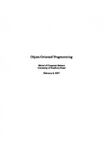
4.2 Kernel Collection The PC++ language begins with a primitive data structure called Kernel collection. The Kernel is the root of the hierarchy of collections. The Kernel can be considered as a simple set of elements which are distributed among processor representatives. The hierarchy of collections derived from kernel is shown in Figure 1. There are four arguments associated with the kernel when we create a new instance of structure. They are the collection variant, the array of processor representatives, the size of the whole collection, and the distribution scheme. The collection variant can be FixedArray, GrowingList, or SynSet. The variant FixedArray means the whole collection can be seen as a distributed array. It is very similar to the conventional array except for that the elements of the collection are distributed among processors representatives. The variant GrowingList means the number of elements in the collection will grow dynamically from parallel phase to parallel phase. If the variant is either FixedArray or GrowingList, the elements are indexed and can be read or written through the indexes. Finally the variant SynSet means a set of unordered elements. The number of elements in a SynSet collection can be either increased or decreased at run time. This kind of structure is particularly useful to served as bu�ers in the producer/consumer problems or the state space of searching problems. The Kernel is the root of the family of distributed collection. The basic, three argument constructor, described in the previous section is inherited from the
Kernel. In addition, there are several other important operators that are found in the Kernel. For example, the method new creates an element and the method vect new creates an array of elements of given distributions. A DOALL operator can be used to cause a particular processor representative or a particular set of processor representatives execute a message concurrently. A DoSubset operator can be used to send a message to a set of elements in the collection. The method get statistics summarizes the information of the current distribution among processors and the method balance balances distribution of the objects among processors.
4.3 Relations between Collections and Elements In this section, we describe the relations between collection and elements. Let's begin with the following de nitions. De nition 1 A collection method is primitive if 1. All the usages of ElementType in the collection method do not requires virtual element methods declared in the MethodOfElement regions. 2. It invokes only primitive collection methods in the current collection. We classify the collection into two categories. One is called a complete element collection and the other is called a eld element collection. Let E be an plain C++ object, and Coll be a collection, we call Coll < E > a eld element collection. If F is an object and declared as class F ElementTypeOf Coll { method_list
};
we called Coll < F > a complete element collection. An element in a complete element collection will
automatically inherit the virutal element methods and instances described in the collection it inherited and the element of a eld element collection will not inherit any virtual instances and methods from the collection. Furthermore, a eld element collection can only invoke the collection methods which are primitive as described in de nition 1. There are three ways that a eld element collection can be formed. The rst way is through the reference of the eld of a complete element collection. For example, in gure 2, W is a complete element collection of type Sequence < element > and W. rst eld forms a eld element collection of type Sequence < int >. Second, a eld element collection can be constructed
Kernel
DistPriorityQueue
BisectedList
DistributedList
DistributedArray
IndexedBinaryTree
Matrix
Figure 1: Collection Hierarchies of Distribution Objects by inheriting the shape from an existing collection instance. For example, W1 is constructed from W and of type Sequence < int > : Finally, we can construct the eld element collection directly if the collection has a constructor which is primitive. In summary, we have the following relations: � If an object class F forms a complete element collection Coll1 < F >, then it can not form another complete element collection Coll2 < F >. � Let E be a plain C++ class, then E can form di�erent kinds of eld element collections. For example, we can have Coll1 < E > and Coll2 < E > at the same time. � A collection Coll can form di�erent complete element collections as well as eld element collections. We can have Coll < E1 >,Coll < E2 >, and Coll < E3 > at the same time.
Collection Sequence : Kernel { Sequence(vconstant *P,vconstant *G, vconstant *D); Sequence(Sequence &ExistingCollection); sorting(); // assume it is primitive MethodOfElement: operator +(); operator =(); operator >(); }; class element ElementTypeOf Sequence{ int first_field, second_field; public: operator +(); operator =(); operator >(); }; Sequence W([MAXPROC],[N],[Cyclic]); foo() { Sequence W1(W); (W.first_field).sorting(); W1= W.first_field + W. second_field; W1.sorting(); }
4.4 Examples
Figure 2: Examples of Di�erent Element Collections
4.4.1 A Smoothing Algorithm
A smoothing algorithm implemented by using a DistributedArray is shown below. Each of the arrays are
distributed by [Block, Block] among processors. This is the Kali notation for partitioning the elements so that blocks of M=MAXPROC by N=MAXPROC elements are assigned to each processor representative. The smoothing algorithm works by having an array of elements each does a local 5-point star relaxation and returns an array of values de ned by the method update. class E ElementTypeOf Darray { float v;
update(){ return(4.0*v -(self(1,0)->v+self(-1,0)->v+ self(0,1)->v+self(0,-1)->v)); } }; Darray A([MAXPROC,MAXPROC],[M,N],[Block,Block]); Darray W([MAXPROC,MAXPROC],[M,N],[Block,Block]); smoothing() { for (i=1; i v = A->update(); A->v = W->v; } }
4.4.2 A Max Finding Algorithm This example illustrates two features of the language. The rst feature is the ability of a collection to inherit algebraic structure. We will de ne a collection called IndexedTree in terms of the DistributedList collection de ned earlier. An indexed tree is a tree where each node has an index to identify it. The root is index 1, the second level has indices 2 and 3, the third level has indices, 4,5,6,7 and, in general, the ith level has indices 2(i?1) through 2i ? 1. The index will be set up properly inside the constructor IndexedTree(). This is done as follows. Collection IndexedTree : DistributedList{ IndexedTree(); MethodOfElement: int this_index; lchild() { return( self(this_index)); } rchild() { return( self(this_index+1)); } }
We leave it to the reader to verify that this de nition of the left and right child will give an ordering consistent with the numbering scheme described above. Our Max-Find will work by distributing the n elements to be searched in an indexed tree. Starting with the bottom level of the tree, each element will ask for the maximum found by its children. class element : ElementTypeOf IndexedTree { float v; public: float local_max(){ if(v < lchild()->v) v = lchild()->v; if(v < rchild()->v) v = rchild()->v; return v; }; }; IndexedTree X([MAXPROC], [N], [Block]); float max_find(N){ for(i = log2(N)-1; i > 0; i--) X.DoSubset([2**i:2**(i+1)-1:1],X.local_max); return(X[1].local_max()); }
The DoSubset operator is the second feature illustrated in this example. The rst parameter is the set of elements over which the second method is to be applied. In this case, our indexing scheme on the tree allows the tree levels to be described as a range of values.
5 Applications
5.1 Matrix Multiplication In this section, we will show a simple matrix multiplication algorithm written in PC++ language. We will begin with the creation of a matrix collection as follows: Collection matrix : DistributedArray { matrix(); matmul(matrix *B1, matrix *C1); MethodOfElement: dotproduct(matrix *B, matrix *C); };
The matrix collection is derived from distributedarray and has a constructor matrix() with three arguments, the processor arrays, the size of global arrays, and the distribution schemes. The operator matmul is to multiply two given matrixes, B and C, and stores the result in the matrix which invokes the computation. This can be done by computing the dotproduct of the ith row of B and jth column of C for every element of which index is (i,j) in the current matrix. This is shown below: matrix::matmul(matrix *B,matrix *C) { this->dotproduct(B,C); }
One thing is worthy of notice is that the dotproduct() described in the collection is a virtual function of the element and will be overloaded when the real element is declared. The invocation of the virtual element method dotproduct() by the collection means the method is applied to all elements of matrix collection. We now show a basic element with a eld name x below: class elem ElementTypeOf matrix { float x; // overload product friend elem operator *(elem *, elem *); elem operator +=( elem &); // overload += dotproduct(matrix *B,matrix *C){ int i,j,k,m; i= thisindex[0]; j= thisindex[1]; m = B->GetSizeInDim(1); for (k=0; k< m; k++) *this += B(i,k)*C(k,j); } }
We have used the power of C++ to overload the operator \*" and \+=" to make it easy to express the dotproduct in the usual manner. Because elem is
declared as an element of matrix, it inherits thisindex from the distributedarray collection. Thisindex will give the index of the current element. operator () is also overloaded in the distributedarray for the access of a particular element given indexes. Finally, we show the main program below: matrix A([MAXPROC],[M,M],[Block,Whole]); matrix B([MAXPROC],[M,M],[Block,Whole]); matrix C([MAXPROC],[M,M],[Block,Whole]); main() { init(); A.matmul(&B,&C); }
This version of matrix multiplication is known as a \point" algorithm, i.e., the basic element contains a single oating point value. The experienced parallel programmer knows that point parallel algorithm perform very poorly on most machines. The reason is that the total amount of communication relative to arithmetic is very high. Indeed, in our example, the references to B(i; j) and C(k; j) in the inner loop may involve interprocessor communication. If we have two interprocessor communications for a single scalar multiply and scalar add, you will not see very good performance. Taking this program almost as is (the only change involved substituting a function name for the operator because overloading is not completely supported at the time of this writing) and running it on the BBN GP1000 we see the problem with a point algorithm very clearly. Table 1 shows the performance of the matrix multiply in mega ops and the speed-up over the execution on one processor. The size of the matrix was 48 by 48. The speed-up reported in this paper is calculated with respect to the execution of PC++ programs on a single node. Fortunately there has been a substantial amount of recent work on blocked algorithms for matrix computation that we can take advantage of. If we replace our basic element in the matrix collection by a small matrix block, we can achieve a substantial improvement in performance. The only di�erence in the two codes is that we have a element of the form class elem ElementTypeOf matrix { float x[32][32]; friend elem operator *(elem *, elem *); elem operator +=( elem &); dotproduct(matrix *B,matrix *C); ... };
The main di�erence is that the overloaded \*" operator is now written as a 32 by 32 subblock matrix multiply. Because this operator has a substantial amount
more work associated with it than the original point operator, we now have enough parallel slack to mask both the latencies of communication and other system overhead. Currently the process of replacing the basic element in the collection by a matrix block is done by programmer. In the future we plan to have it done automatically by the compiler in most of the cases. We now list the GP1000 times in the Table 2 for a matrix of size 1024 by 1024. Running this same blocked code on the 12 processor I860 based Alliant Fx2800 we have the results in the Table 3. It must be noted that we cheated slightly in reporting the speedup number for the 2800. The actual speed of this code on one processor is 3.98 M ops when run with the I860 cache enabled. Unfortunately, in concurrent mode the caches are all disabled so we have based the speedups on the one processor concurrent mode times. Many readers may be concerned that the M op numbers reported above are very small relative to the actual peak rate of the machine. In fact, for the BBN GP1000, the node processor is the old M68020 which is not very fast. The numbers above are very good for that machine. For the I860 we see two problems. First the Alliant code generator is not yet mature and the cache problem must be xed before we can get better numbers. However there is another solution to this problem. Because of the modular nature of the PC++ code it is very easy to use assembly coded kernels for operations such as the 32 by 32 block matrix multiply. To illustrate this point we have done exactly this for the old Alliant FX/8 with 4 processors. The results are shown in the Table 4. These numbers are very near the peak speeds of 32 M ops for this machine. We intend to build a library of hand coded assembly routines for the I860 processor to speed performance on standard collections running on the Fx2800 and the Intel IPSC.
5.2 PDE Computations: The Conjugate Gradient Method One of the most frequently used methods of solving elliptic partial di�erential equations is the method of conjugate gradients (CG). In this example, we will look at a simple version of CG for a two dimension nite di�erence operator. We begin by de ning a collection called Grid to represent a simple M by M mesh on the unit square. The nite di�erence approximation to the partial di�erential operator is given by the equation A�u= f
p=1 p = 2 p = 3 p = 4 p = 6 p = 8 p = 12 p = 16 M ops 0.0041 0.0073 0.0104 0.01298 0.01087 0.01435 0.0083 0.0081 Speed-up 1.0 1.78 2.54 3.165 2.65 3.5 2.02 1.97
Table 1: Pointwise Matrix Multiply of size 48 by 48 on the GP1000 p=1 p = 2 p = 3 p = 4 p = 6 p = 8 p = 12 p = 16 M ops 0.0775 0.1547 0.2319 0.3091 0.4627 0.6166 0.9137 1.21187 Speed-up 1.0 1.99 2.99 3.98 5.97 7.95 11.8 15.6
Table 2: Blocked Matrix Multiply of size 1024 by 1024 on the GP1000 where u is a two dimensional array of unknowns and f is a two dimensional array of \right hand side" values. Each component of u and f is associated with one vertex in the grid. The operator A is taken to be a simple nite di�erence operator of the form A(ui;j ) = ui;j ? 0:25 � (ui?1;j +ui+1;j +ui;j ?1 +ui;j +1): The boundary conditions will be that u is zero along the boundary of our grid. Our rst approach to this problem will be to have each element of the Grid collection correspond to one vertex in the grid. This vertex element will contain one component of each of u, f and four other arrays e, p, q and r needed by the CG algorithm. Because of local structure of the nite di�erence operator, each vertex element must be able to access its neighbors to the north, south, east and west. Fortunately, the Collection DistributedArray has, in two dimensions, the self(i,j) operator take two parameters corresponding to displacements along the two dimensions of the array. Consequently, the operator A is almost a trivial generalization of the local average operator illustrated in section 4.1. The only major di�erence is that each element must know when it is on the boundary of the collection so that the boundary conditions may be applied. Because this is a property of the global topology of the grid, we will put a set of special boolean functions, top edge(), bottom edge(), left edge, right edge in the collection that returns 1 if an element is on the corresponding boundary. Our Grid collection now takes the form Collection Grid: DistributedArray{ public: Grid(vconstant *P,vconstant *G,vconstant *D); double dotprod(int, int); MethodOfElement: int top_edge() {if (thisindex[0]==0)return 1;else return 0;} int bottom_edge() {if (thisindex[0]==M-1)return 1;else return 0;}
int left_edge() {if (thisindex[1]==0)return 1;else return 0;} int right_edge() {if (thisindex[1]==M-1)return 1;else return 0;} double localdot(int, int); };
The CG algorithm requires that we frequently use the inner product operation X dotprod(u; f) = ui;j � fi;j : i;j
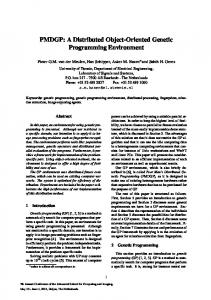
Computation of the dotprod function requires that we form the local products (which we compute using a element function localdot() and do a global sum over the entire Grid collection. (The protocol for using the dotprod function is to give each variable in the local element a unique integer identi er. The call dotprod(3,2) will cause the element method localdot(3,2) to be called which, in turn, should compute the products of the 3rd and 2nd variables to be multiplied. A more elegant solution exists, but was not used in the experiments described here.) At this point it is not hard to complete this \point" version of the CG algorithm, but, just as with the point version of matrix multiply, we will nd that the communication between elements on di�erent processors will dominate the execution time. Again, to achieve better parallel slackness, we can block the computation as illustrated in Figure 3. Each block is in fact a small subgrid of size N by N. If we now de ne our basic element of the Grid collection to be such a subgrid we have class SubGrid ElementTypeOf Grid{ public: float_array f[N][N], u[N][N],e[N][N]; float_array p[N][N], q[N][N], r[N][N]; void Ap(); double localdot(int, int);
p=1 p = 2 p = 3 p = 4 p = 6 p = 12 M ops 2.26 4.26 6.48 8.56 12.78 22.81 Speed-up 1.0 1.88 2.86 3.78 5.65 10.09
Table 3: Blocked Matrix Multiply of size 1024 by 1024 on the FX2800 p=1 p = 2 p = 3 p = 4 M ops 7.91 15.69 23.11 30.74 Speed-up 1.0 1.98 2.92 3.88
Table 4: Blocked Matrix Multiply of size 1024 by 1024 on the FX/8 with assembly BLAS3 };
where oat array is a C++ class that has all the basic arithmetic operators overloaded for \vector" operations. Everything we have said about the point algorithm holds for the blocked \subgrid" algorithm, except our grid will actually be of size N � M by N � M. The body of the CG computation is shown below. Grid G([MAXPROC], [M,M], [Block,Block]); conjugategradient(){ int i; double gamma, alfa, tau, gamnew, beta; G.Ap(); // q = A*p G.r = G.f - G.q; gamma = G.dotprod(R,R); G.p = G.r; for(i = 0; i < M*N*M*N && gamma > 1.0e-12 ; i++){ G.Ap(); // q = A*p tau = G.dotprod(P,Q); // tau = if(tau == 0.0) {printf("tau = 0\n"); exit(1);} alfa = gamma/tau; G.r = G.r - alf*G.q; gamnew = G.dotprod(R,R); // gamnew = beta = gamnew/gamma; G.u = G.u + alfa*G.p; G.p = G.r + beta*G.p; gamma = gamnew; } }
The performance of this algorithm for the GP1000 is shown in the Table 5 for di�erent block sizes and di�erent distribution schemes. (All times in this section are in seconds.) Observe that if the Distribution is [Block,Block], the number of processors must be a square for small values of M. Also, if when N = 128 the problem was too big to run on 1 processor, so a speed-up of 4 was assumed on 4 processors. Clearly from this table we see that a block size of 64 is su�cient to get most of the performance out of this program.
In the case of the Alliant Fx2800 we have the results in the Table 6. In this case, increasing the block size does not help the Fx2800 because, unlike the matrix multiply example, the CG algorithm must sweep over all the subblocks before one is reused. This causes the Alliant cache to over ow and we are then limited by the bus bandwidth to the speed-ups above.
5.3 A Fast Poisson Solver An important special case in the numerical solution of PDEs is the solution to the Poisson equation @ 2 u + @ 2 u = f: @x2 @y2 The fast Poisson solver operates by exploiting the algebraic structure of the nite di�erence operator A associated with the di�erential operator. A is just the 5-point stencil described above. Assume a computational grid of size n by n where n = 2k + 1 for some integer k. The basic idea is to observe that A can be factored as A= Q�T �Q where Q is an block orthogonal matrix and T is block tridiagonal. It turns out that each block of Q corresponds to a sine transform along the columns of the grid and the tridiagonal system that compose the blocks of T are oriented along the rows of the grid. Solving the equation A � U = F becomes U = Q � T ?1 � Q � F: Our strategy for programming this example is as follows. We will represent the grid arrays U and F each as a linear array of vectors. A vector will be a special class with a number of builtin functions including FFTs and sine transforms, and the linear array will be
oooo
oooo
oooo oooo
oooo
oooo
oooo
oooo
oooo
oooo
oooo
oooo
oooo
oooo
oooo oooo
oooo
oooo
oooo
oooo
oooo
oooo
oooo
oooo
oooo
oooo
oooo oooo
oooo
oooo
oooo
oooo
oooo
oooo
oooo
oooo
Blocked grid with local subgrids and edge vectors for neighbor communication
Partitioned Grid
Figure 3: Blocked Subgrid Structures for the Grid Collection M=16,N=16, Block,Whole Time Speed-Up M=4,N=64, Block,Block Time Speed-Up M=4,N=128, Block,Block Time Speed-Up
p=1 83.15 1.0 p=1 80.13 1.0 p=1 **** 1.0
p=2 42.68 1.94 p=2 ||p=2 ||-
p=4 21.85 3.80 p=4 20.5 3.9 p=4 85.06 4.0*
p=8 11.69 7.11 p=8 ||p=8 ||-
p = 16 8.14 10.21 p = 16 6.99 11.46 p = 16 28.67 11.9
Table 5: 20 CG Iterations on Grid of Size 256 by 256 on the BBN GP1000. a collection with a built in function to solve a tridiagonal system in parallel across the collection. We will associate the columns of the grid with the vectors and the row dimension will go across the collection. More speci cally we de ne our collection as Collection LinearArray: DistributedArray{ ... public: CyclicReduction(ElementType a,ElementType b); };
where the method CyclicReduction(a,b) solves a system of tridiagonal equations of the form b � xi?1 + a � xi + b � xi+1 = yi for i = 1; n, where the values yi are the initial elements of the collection which are overwritten by the results xi . The exact code for this O(log(n)) parallel tridiagonal system solver is void LinearArray:: CyclicReduction(ElementType x,ElementType y){
int i, s; ElementType *a, *b, c; a = new ElementType[log2(n)]; b = new ElementType[log2(n)]; a[0] = x; b[0] = y; // forward elimination for(s = 1; s < n/2; s = 2*s){ c = b[s]/a[s]; b[s+1] = -c*b[s]; a[s+1] = a[s] +2*b[s+1]; Y.DoSubset(i, [2*s: n-1: 2*s], (*this)(i)+=-c*((*this)(i-s))+ (*this)(i+s)); } // backsolve for(s = n/2; s >= 1; s = s/2) Y.DoSubset(i,[s: n-1: 2*s], (*this)(i)+=-b[s]*(*this)(i-s)+(*this)(i+s))/a[s]); }
In this case, the DoSubset operator evaluates the expression argument for each instance of the variable i in the given range. (This version of the DoSubset operator is not yet implemented, so the in the actual code a more messy, but functionally identical form is used.) Notice that we have left the element type unspeci ed. In order for this algorithm to work properly
M=12,N=32, Block,Whole p = 1 p = 2 p = 3 p = 4 p = 6 p = 12 Time 31.1 16.69 11.52 8.94 6.35 3.63 Speed-Up 1.0 1.86 2.69 3.47 4.89 8.56
Table 6: 384 CG Iterations on Grid of size 384 by 384 on the Fx2800. all we need is an element with the basic arithmetic operators \*", \+", \/" and \+=". Because we want each element to represent one column of the array we can use class vector ElementTypeOf LinearArray{ int n; // size of vector. float *vals; // the actual data. public: vector(); vector(int size); float &operator [](int i){ return vals[i]; } vector &operator =(vector); vector operator *(vector); vector operator +(vector); friend vector operator *(float, vector); void SinTransform(vector *result); };
The complete code for the Fast Poisson Solver now takes the form shown below. We declare three linear arrays of vectors: one for the \right hand side" F, one for the solution U, and one for a temporary Temp. We rst initialize a pair of vectors of special coe�cients a and b. Next we do a sine transform on each component of F leaving the results in Temp. Next we apply the cyclic reduction operator to solve the tridiagonal systems de ned by the rows of the matrix. Finally, we apply the sine transforms again to each column. LinearArray F([MAXPROC],[n+1],[Block]); LinearArray Temp([MAXPROC],[n+1],[Block]); LinearArray U([MAXPROC],[n+1],[Block]); poisson(int n){ vector a(n+1); vector b(n+1); for(i = 1; i < n; i++){ a[i] = 4-2 *cos(i*pi/n);b[i] = -1; } F.SinTransform(Temp); Temp.CyclicReduction(a,b); Temp.SinTransform(U); }
Notice that the cyclic reduction operation solved the tridiagonal equations as a \vector" of tridiagonal equations parallelized across processors, i.e. each processor participates in the solution of each equation. Furthermore it is at this stage where we do most of the inter processor communication. On the other hand,
locality has been preserved for each sine transform, because we have parallelized that as a set of independent transforms each done with a single processor. We have executed this code on both the alliant Fx2800 and the BBN GP1000 and the results are shown in Table 7.
5.4 0/1 Knapsack Problem In this section we show an implementation of 0/1 knapsack problems by using distributed array collections based on the algorithm developped by Sahni[11]. The one-dimensional 0/1 knapsack problem Knap(G; C) can be de ned as follows: Given a set of m di�erent objects and a knapsack, each object i has a weight wi and a pro t pi, and the knapsack has a capacity C. C, wi, and pi are all positive integers. The problem is to nd a combination of objects include in the knapsack such that P TotalProfit = mi=1 pizi is maximized P subject to mi=1 wizi � C � object i is included where zi = 10 ifotherwise The algorithm we show here is to decompose the original problem into subproblems of smaller size, to solve all subproblems in parallel and nally combine all partial solutions into the original solution. Our algorithms will only nd out the solution of TotalPro t but not the solution vector zi . The solution vector zi can be found without changing the idea of the algorithm by saving all the history of pro t vectors and backtracking from TotalPro t[11]. The algorithm can be divided into three phases. In the rst phase of the computation, we will set up a distributed array of m di�erent objects and a distributed array of #proc pro t vectors. This can be done by the followings. class int }; class
object ElementTypeOf Darray{ weight,profit; ProfitVect ElementTypeOf Darray {
Fx2800, Time Speed-Up GP1000, Time Speed-Up
p=1 7.51 1.0 p=1 70.48 1.0
p=2 3.85 1.95 p=2 35.66 1.97
p=3 2.63 2.86 p=3 24.03 2.94
p=6 1.40 5.36 p=6 12.65 5.57
p = 12 0.723 10.38 p = 12 p = 24 7.48 6.36 9.42 11.08
Table 7: Fast Poisson Solver on a 256 by 256 grid. int v[C+1]; combine(int stride); }; Darray G([MAXPROC],[m],[Block]); Darray S([MAXPROC],[MAXPROC],[Block]);
Next, we have each processor representative in the distributed collection G perform dynamic programming on its local collection Knap(Gi ; C). This can be done by employing the DOALL operator. A DOALL operator will send a message dynamic knapsack() to each processor representative in the collection G and have the set of processor representatives in G execute the message simultaneously. Therefore each processor representative i of collection G will solve Knap(Gi ; C) by applying dynamic programming and get a pro t vector stored in the ith pro t vector of S respectively. The pro t vector of size C + 1 stands for the current best TotalPro t under the capacity from 0 to C. The nal stage is the combining stage. The combining process combines the resulting pro t vectors. Let b,d be two pro t vectors for Knap(B; C) and Knap(D; C) such that B \ D = �, Then pro t vector e of G(B [ D; C) can be obtained in the following way: e = combine(b; d) where ei = max0�j �i fbj + di?j g; for i = 0; 1; :::; C The method combine is built as a method of the ProfitVector. It takes an argument stride to know what element it will be combined with. For example, combine(j) will result in the combining of current ProfitVector and self(j). Notice that self() is treated like a pointer (in the C sense) into our distributedarray and that we can add o�sets to access the eld variables of sibling Pro tVector in the collection. The combining process can be represented as a tree. Each time after the combining the number of active Pro tVector is reduced to half of the original number. The new pro t vector is always stored in the ProfitVector with lower index number in the distributed array collection S. The procedure is repeated until the nal pro t vector is constructed. Finally, we show
the main program which includes the dynamic programming stage and the combining stage below. The DoSubset operator in the program is used to send the message combine() to an index set of Pro tVector elements in the collection. The experimental result with m=16*1024, C=400 is also shown in the Table 8. main() { int stride,i,p; G.DOALL(dynamic_knapsack); p = S.max_elements(); for (stride=i=p/2;i>=1;i=i/2,stride=stride/2) S.DoSubSet([0:i-1:1],S.combine,stride); }
5.5 Traveling Salesman Problem In this section, we will discuss the traveling salesman problem as a representative example for parallel branch and bound. The traveling salesman problem can be stated as follows: Given a set of cities and inner-city distances, nd a shortest tour that visits every city exactly once and returns to the starting city. The problem can be solved using branch and bound algorithm. The program studied here will be based on LMSK algorithm[8][10]. Our PC++ program uses the collection called DistributedPriorityQueue from PC++ collection libraries to manage the searching state space. The experiments are conducted both on Alliant/FX-2800 and BBN GP 1000 machines. The LMSK algorithm works by partitioning the set of all possible tours into progressively smaller subsets which are represented on the nodes of a state-space tree and then expanding the state space tree incrementally toward the goal node using heuristic to guide the search. A reduce matrix is used to calculate the lower bounds for each subset of tours. The bound guides the partitioning of subsets and eventually identify an optimal tour { when a subset is found that contains a single tour whose cost is less than or equal to the lower bounds for all other subsets, that the tour is optimal. Our algorithm will use DistributedPriorityQueue collections to manage the creation and removement of state nodes in the searching space. Every element
M=16k, Capacity=400 p=1 p=2 Alliant FX/8 time(seconds) 99.23 50.09 speed-up 1 1.98 Alliant FX/2800 time(seconds) 12.58 6.39 speed-up 1 1.97 BBN GP1000 time(seconds) 125.84 63.85 speed-up
1
1.97
p=4 p=8 p=16
26.23 3.78 3.30 1.79 3.81 7.02 33.36 18.58 3.77 6.77
12.15 10.35
Table 8: 0/1 Knapsack Problem of the collection will be a state in the state space tree. The state element is shown below: class state ElementTypeOf DistPriorityQueue{ int lower_bound,rank, reduce_matrix[N][N]; public: int cost(){return lower_bound;}; int priority() {cost();} expand(DistPriorityQueue *Space); };
The priority() function above is a function to overload the virtual function priority() described as an abstraction in the DistPriorityQueue to decide the priority of elements in the collection. The expand() method will select a splitter and expand the current state into two states, each with smaller subsets of tours. If any of the new states is a complete solution, the expand function will compare it with the current best solution and save it if it is better. If the new states are not complete solutions, it will be stored in the Space collection. We will create two collections, Space and Working Queue. Every time we move a certain number of nodes with lower cost from Space queue to Working Queue. Then we expand all the state nodes of the Working Queue parallel by invoking the expand() operator of the state. The program will stop when it eventually identify an optimal tour. The experimental result on Alliant FX/8, Alliant FX/2800, and BBN GP1000 is shown in the Table 9. Let's assume that Texpand be the average time needed to compute the LMSK heuristic of the generated nodes in each iteration and Taccess be the average time spent in accessing the DistPriorityQueue per node expansion(storing new nodes). Then the speed up is fairly linear for small number of processors, but saturates at Texpand =Taccess. Our current implementation for DistributedPriorityQueue is still very preliminary, so the overhead in the access of the queue is relative large. The saturation appears when processor number is more than 8. In the future, we plan to improve it based on high-performance concurrent queues[9]. One
thing to notice is that the change of queue implementation in the future will not change user's program, since the collection abstraction hides the low level details.
6 Conclusion In this papers, we have presented an objectoriented, parallel programming paradigm, called the distributed collection model and an experimental language PC++ based on the model. In the distributed collection model, programmers can describe the data distribution of elements among processors to utilize memory locality and a collection construct is employed to build distributed structures. The model also supports the express of massive parallelism and a new mechanism for building hierarchies of abstractions. We have also described our experiences with application programs and the performance results in the PC++ programming environments. There are still many challenges remaining in compiler optimization and runtime support for the distributed collection model and PC++ language. The problems include optimizing the cost of the access functions for distributed collections, automatically replacing the basic element in the collection by a matrix block of elements, and the choice between locality and randomization. We are investigating these issues. In addition to that, we are building a rich set of abstractions of distributed data structures as libraries. This will be an important step for a better parallel programming environment for users as well as for us to understand the characteristics and necessary primitive functions of the model.
References [1]
William L. Bain Indexed, Global Objects for Distributed Memory Parallel Architectures,
Number Of City = 25 Alliant FX/8 time(seconds) speed-up Alliant FX/2800 time(seconds) speed-up BBN GP1000 time(seconds) speed-up
p=1 p=2 p=4 p=8 p=12
60.04 1 3.29 1 81.26 1
32.61 18.55 1.84 3.23 1.90 1.16 0.96 1.73 2.83 3.40 45.72 28.60 20.75 1.77 2.84 3.92
1.08 3.02 21.68 3.74
Table 9: Traveling Salesman Problem with 25 Cities
[2]
[3] [4] [5]
Proceedings of the ACM SIGPLAN Workshop on Object-Based Concurrent Programming, pp. 95-98, Sigplan Notices, Volume 24, Number 4, April 1989. Andrew A. Chien and William J. Dally. Concurrent Aggregates (CA), Proceedings of the Second ACM Sigplan Symposium on Principles & Practice of Parallel Programming, Seattle, Washington, March, 1990. Nicholas Carriero and David Gelernter. Linda in Context, Communications of the ACM, Vol. 32, No. 4, April, 1989 William Dally. A VLSI Architecture for Concurrent Data Structures, Kluwer Academic Publishers, Massachusetts, 1987 Charles Koelbel, Piyush Mehrotra, John Van Rosendale. Supporting Shared Data Structures on Distributed Memory Architectures, Technical Report No. 90-7, Institute
[6]
[7] [8]
[9]
for Computer Applications in Science and Engineering, January 1990. J. T. Kuehn and Burton Smith. The Hori-
zon Supercomputer System: Architecture and Software, Proceedings of supercomput-
ing '88, Orlando, Florida, November 1988. Bjarne Stroustrup. The C++ programming Language, Addison Wesley, Reading, MA, 1986 J. D. C. Little, K. Murty, D. Sweeney, and C. Karel. An Algorithm for the Traveling Salesman Problem, Operations Research, No 6, 1963. V. N. Rao and V. Kumar. Concurrent Access of Priority Queues, IEEE Transactions on Computers, Vol 37, No 12, Dec 1988.
[10]
[11]
[12]
V. Kumar, K. Ramesh, and V. N. Rao. Parallel Best First Search of State Space Graphs: A Summary of Results, Proceed-
ings of the 1988 National Conference on Arti cial Intelligence(AAAI-88), 1988. Jong Lee, Eugene Shragowitz, and Sartaj Sahni. A Hypercube Algorithm for the 0/1 Knapsack Problem, Proceedings of the 1987 International Conference on Parallel Processing, pp. 699-706, 1987. Marc Shapiro, Yvon Gourhant, Sabine Habert, Laurence Mosseri, Michel Ru�n, and Celine Valot SOS: An Object-Oriented Operating System - Assessment and Perspectives, Computing Systems, Vol. 2, No
4, pp. 287-337, Fall 1989.