counterexample is due to Naimann and Wynn, who also have an algebraic topology ..... censoring rule (1.12) as a function of the number of painted grid-points.
On some weighted Boolean models. Wilfrid S. Kendall ABSTRACT An overview is given of some recent work (joint with Adrian Baddeley of Perth and Colette van Lieshout of Warwick) on a new class of random point and set processes, obtained using a rather natural weighting procedure employing quermass integrals. The concept of exact (or perfect) simulation of point processes is then introduced, and a discussion is given of possibilities for perfect simulation of quermass weighted processes.
1 Introduction. This short paper is a progress report on some recent work of mine (partly in collaboration with Adrian Baddeley of Perth and Colette van Lieshout of Warwick); concerning new models for point processes and random sets, and the application to them of a new technique for \exact" or \perfect" simulation.
2 A brief overview of quermass-interaction processes In this section we review the idea of weighting point processes and random sets using quermass integrals. Recall Baddeley and Van Lieshout's de nition [BvL95] of an area-interaction point process: this may be viewed as the point process produced by the germs of a Boolean model � under the weighting
?area(�) : (1:1) In the case > 1 this was introduced by Widom and Rowlinson [WR70] in statistical physics as the \penetrable sphere model". In its simplest form the process is de ned in a bounded planar region W ; the grains of the Boolean model are chosen to be disks of xed radius r; and therefore the resulting point pattern x � W has probability density p(x) with respect to a Poisson process of intensity (say) in W , given by S
?area( f ( ): 2xg) : (1:2) p(x) = Z ( ; ) B xi ;r
xi
2
Wilfrid S. Kendall
Here B (x ; r) is the disk of radius r and centre x , and Z ( ; ) is the normalizing constant (the task of evaluating Z ( ; ) is an intransigent computation of an exponential moment of coverage for the corresponding Boolean model! See for example [Hal88]). Clearly one can also view this weighting as producing a weighted Boolean model of a rather simple form, if attention is focused on the random set produced by the union of the grains. If attention is focused on both the individual grains and the germs (possibly deducible from the grains, as would be the case for germs the centre of disk-shaped grains) then we speak of a weighted germ-grain model. Although in the following we will frequently focus on the point process, always in the background will be the weighted Boolean model, thus justifying the title of this paper. Parameter values > 1 here correspond to clustering or attraction between germs; values < 1 correspond to orderliness or repulsion. Baddeley and Van Lieshout note a delightful interpretation in terms of behavioural biology: if the points of x were to correspond to locations of animals in a herd then > 1 corresponds to the animals seeking to minimize their regions of vulnerability (\sel sh herd"), while < 1 corresponds to maximizing their regions of in uence. More generally one can generalize to higher-dimensional cases, to random or varying compact grains, or by replacing area by some other Radon measure. Baddeley and Van Lieshout establish existence and extension properties for the density, describe simulation methods based on rejection-sampling and on spatial-birth-and-death techniques, and discuss issues of inference. In particular if the grains are uniformly bounded then (in the bounded window case) the area-interaction is always stable in the sense of Ruelle [Rue69], namely, p(x) � constant � a (x) (1:3) for some constant a > 0, where n(x) is the number of points in the pattern x; from which there follows easily the niteness of the normalization constant Z ( ; ) and hence other useful properties. More recently Baddeley, Kendall and Van Lieshout [BKvL96] have considered the following generalization: proceed as above but weight the realization of the Boolean model � by an exponential of a quermass integral extended to the convex ring, rather than an exponential of the area functional: 2 (1:4)
? (�) : Of course case r = 0 simply gives the area-weighted interaction. Case r = 1 is equivalent to weighting by the perimeter length(@ �); case r = 2 is equivalent to weighting by the Euler functional i
i
n
Wr
�(�) = (number of components of �) ? (number of holes of �) : (1:5)
1. On some weighted Boolean models.
3
Motivations (discussed in [BKvL96]) include 1: if the area-interaction is viewed as a weighting applied to a Boolean model then these are obvious and simple generalizations; 2: they give a new and simple class of point process models; 3: there is a loose relationship between the inclusion-exclusion relation, satis ed by the quermass integrals W , and a weak Markov-like property. At least from a theoretical point of view, the perimeter-weighted case r = 1 adds little new, largely because both W12 and W02 are positive functionals and so for both r = 0 and r = 1 we have (1:6) 0 � W 2 (K1 [ K2 [ ::: [ K ) � n � max W 2 (K ) : Consequently the resulting interactions are Ruelle-stable if the grains are convex and uniformly bounded, and so the corresponding normalization constants are nite and the densities well-de ned. It is an interesting question as to how the resulting point processes and random sets might di�er, and we hope to investigate this soon at Warwick, using \perfect simulation" methods to be described below. The planar case r = 2, of Euler weighting, is much more interesting, since the Euler characteristic is not non-negative! It satis es the inclusionexclusion relationship �(K1 [ K2 ) = �(K1 ) + �(K2 ) ? �(K1 \ K2 ) (1:7) (together with the relationship �(K ) = 1 for convex compact K and �(;) = 0, this typically provides the most convenient way in which to compute � (�)!) but negative values of �(�) are possible (consider the case of a number of disks arranged in an overlapping gure-of-eight, as in Figure 1). Consequently the Euler-interaction is Ruelle-stable for < 1 because of �(K1 [ K2 [ ::: [ K ) � n (1:8) (for convex compact K ) but need not be stable for > 1. Most of the work of [BKvL96] is concerned with elicitation of conditions on the grains under which the Euler weighting is always stable: namely either (a) the grains are all disks (not necessarily of xed radius) or (b) the grains are all polygons which are uniformly neither too small nor too \needle-like". It is also intended to investigate these cases further at Warwick using simulation methods related to those described below, but, as we will see, these processes will be harder to study. Of course it is possible to generalize area- and perimeter-weighting in another way, by replacing the convex ring extensions of the quermass integrals by the positive extensions [Mat75]. Exactly because these extensions are positive, they do not present the same di�culties over stability. d r
n
r
i
i
i
i
n
i
r
4
Wilfrid S. Kendall
FIGURE 1. Example in which the Euler constant is negative: nine disks are arranged in a gure-of-eight, such that there are ten non-void pairwise intersections and no other non-void intersections. Consequently the Euler characteristic is 9 ? 10 = ?1.
We note in passing that the higher-dimensional case is far more involved. Some stability results carry over from W22 to W23 (more generally, W2 for d = 3; :::) by a stereological argument (namely stability for grains which are disks of varying radius), but [BKvL96] describe counterexamples to show that the 3-space interaction ? 33 (�) cannot be stable for > 1 if4 grains are balls of strictly varying radius and the 4-space interaction ? 4 (�) cannot be stable for > 1 even if grains are balls of constant radius (this second counterexample is due to Naimann and Wynn, who also have an algebraic topology proof of stability for the planar interaction ? 22 (�) and grains which are disks of general radius, based on their work [NW92, NW96]; 3 (�) ? 3 Naimann also separately derived the counterexample). It is still an open question whether the 3-space interaction ? 33 is stable for grains which are balls of constant radius. d
W
W
W
W
W
3 A brief overview of perfect (or exact) simulation A remarkable recent paper by Propp and Wilson [PW96] shows how in certain cases it is practical to sample exactly from the equilibrium distribution of a Markov chain with large state space (such as the Ising model). This has now been extended to deal with spatial point processes in two di�erent ways. Haggstrom et al [HvLl96] use the rejection-sampling idea in [BvL95] to produce a Gibbs sampler which they then use to investigate attractive area-interaction point processes and other related point processes.
1. On some weighted Boolean models.
5
On the other hand [Ken97] explains how \exact sampling" can be arranged for the spatial birth-and-death approach to simulation of area-interaction point processes: this second approach is based on a space-time Boolean model and can deal with the repulsive case and generalizes to yield \exact simulation" techniques for quite general point processes with bounded local energy (though in the repulsive cases it will be very slow when the repulsive interaction is strong and the intensity is large). In [Ken97] there is given the simplest possible example of a Propp-Wilson exact sampling algorithm, using a two-state Markov chain with transition matrix � � 0 1 P = : 1=2
1=2
Rather than repeat that example here, instead we describe how to do exact sampling for a suitable (one-dimensional) birth-death process. Of course in this case it is trivial to nd the equilibrium distribution by direct computation! but a description of this trivial case will allow the basic simplicity of the Propp-Wilson idea to shine forth, and has the added advantage of being closely related to the approach of [Ken97]. Suppose then that X is a continuous-time Markov chain on the positive integers, with transition rates given by X !X +1 at rate �(X ) ; X !X ?1 at rate �X : (1.9) Thus each individual departs at constant rate �, and individuals arrive at rate �(X ) depending on the current population. We suppose that the overall birth rate is a bounded increasing function of the total population and is strictly positive: 0 < �(0) � �(x) � �(x + 1) � � : (1:10) We could for example think of incidences of an infectious disease, with cases arising from infection from without the population at a constant positive rate �(0), and arising further from within-population infection at a variable rate �(x) ? �(0)). Note however the monotonicity requirement, which is not found in realistic epidemic models. It is intuitively clear that X is dominated by a simpler process Y for which each individual dies at constant rate � as before, but for which individuals arrive at a constant rate �. This leads to transition rates as follows: Y !Y +1 at rate � ; Y !Y ?1 at rate �Y : (1.11)
6
Wilfrid S. Kendall
The domination of X by Y can be expressed as a coupling as follows. The process Y satis es detailed balance, with an equilibrium distribution which is Poisson of mean �=�. Therefore Y is reversible in time when in statistical equilibrium. We simulate the nal value Y0 and then simulate Y backwards in time over the range [?T; 0], attaching an independent uniform [0; 1] random variable as a mark to each arrival or departure time t (that is, each t such that Y = Y ? � 1). We can arrange this so that if we need to extend backwards in time to a simulation over [?S ? T; 0] then we just continue the [?T; 0] simulation backwards by a further time interval of length S . For each xed initial ?T we can simulate X with an initial value X? � Y? as follows: if there is a Y -arrival at t (so Y = Y ? + 1) then make it also be an X -arrival (so X = X ? + 1) if and only if the mark U at time t satis es U � �(X ? )=� : (1:12) On the other hand if there is a Y -departure at t (so Y = Y ? ? 1) then make it also be an X -departure (so X = X ? ? 1) if and only if the mark U at time t satis es X? : (1:13) U � Y t
t
T
T
t
t
t
t
t
t
t
t
t
t
t
t
t
?
t
t
Note that if X ? = 0 then no departure can occur for X ! It is easily checked that this is a construction of X with the rates as given above in equation (1.9). Furthermore, the monotonicity condition (1.10) means that once the realization is xed then X is a monotonic function of the initial condition X? (this follows inductively from the censoring rules (1.12) and (1.13)). Consequently, for any xed initial ?T there is a maximal such process (say X (? max) , with X?(? max) = Y? ) and a minimal such process (say X (? min) , with X?(? min) = 0). Figure 2 illustrates the construction of X (? max) and X (? min) from Y and the marks. From the construction we have t
t
T
T;
T;
T
T
T;
T;
T T;
T;
0 = X?(?
min)
T;
T
� X?(? ? � X?(? ? S
T
S
T
min)
T;
max)
T;
� �
X?(? max) T;
T
= Y? (1.14) T
whenever ?S ? T � ?T . (It is vital for this that the same uniform [0; 1] marks remain attached to each Y -arrival and Y -departure.) On the other � hand,� almost surely there is some initial ?T � such that X0(? min) = X0(? max) (this certainly happens if Y vanishes at some time in the range [?T � ; 0], which will eventually occur for large enough T � , but this is not a necessary condition). Consequently for any ?S < ?T � we have T
T
;
;
1. On some weighted Boolean models.
Time -T
7
Time 0
FIGURE 2. Construction of maximal process (solid stepped line) and minimal process (broken stepped line) from Y (arrowed segments indicate periods between arrivals and departures of individuals) and the marks (diagonal lines growing from arrivals: shorter marks are more likely to be censored). In the example coalescence has already occurred. � � X0(? min) = X0(? min) ; intuitively speaking, X0(? min) is the result of a virtual simulation of the X -process from time ?1. Since we know from basic theory that the X -process converges to an S;
T
;
T
;
equilibrium distribution, it follows easily that once � X0(? min)
�;
= X0(? max) (1:15) then the common value must be an exact sample from this equilibrium distribution. This is the Propp-Wilson idea for exact simulation: the algorithm is simply to extend the simulation backwards till ?T � is su�ciently negative for the condition (1.15) to hold. (Of course this also allows us to simulate a stationary version� of X : just continue a simulation forward in time from initial value X0(? max) .) As we have noted, in this case it would be far simpler to simulate directly from the known equilibrium distribution of X . However it is not hard to modify this construction to apply to spatial birth-and-death processes which satisfy an attractivity condition (just add a randomly chosen location to each arrival incident, and alter the censoring rule (1.12) to depend appropriately on the current con guration of points). Direct simulation of such point processes is typically not feasible, so the above approach o�ers a real advantage! The details and simulation results are worked out for the area-interaction point process in [Ken97], in which a space-time Boolean model replaces the immigration-death process Y above. In the next section we discuss the extent to which this generalizes to quermass-interaction proT
T
;
;
T
8
Wilfrid S. Kendall
cesses (for example). If the overall infection rate �(x) is decreasing in x then monotonicity no longer applies. However we can then sandwich all realizations over [?T; 0] between a coupled pair of processes X (? � min) , X (? � max) evolving according to the paired censoring rule (replacing the arrival rule (1.12)) T
� � X (? max) = X (?? max) + 1 � � X (? min) = X (?? min) + 1 T
;
T
t
T
t
;
t
;
T
t
;
;
T
;
if U � �(X (?? if U � �(X (??
T
t
t
� ;min)
T
t
t
)=� ; )=�
� ;max)
(1.16)
and using the original rule (1.13) for departures. Because �(x) is now decreasing it follows that� X , the \virtual� process from time ?1", is sandwiched between X (? min) and X (? max) , and this enables perfect simulation as before. Again it is not hard to modify this for spatial birth-and-death processes which satisfy a repulsivity condition; [Ken97] gives details and simulation results for the area-interaction point process. This will work well for \reasonable" parameter values (typically, parameter values for which a particular kind of percolation does not occur). Notice that, in either case, if the simulation were conducted forwards in time till coupling occurred then we would obtain a biased sample (coupling will be� more likely to occur at low values of Y and thus of X (? � min) , X (? max) ). For the same reason it is important that we extend the simulation backwards in time, rather than discard the [?T; 0] simulation and start afresh with the [?S ? T; 0] simulation. Finally, note the following practical aspect of actual implementation of this algorithm. Although the sampling is exact if the algorithm is carried to completion, the amount of time required for this is random. Therefore in practical circumstances one must admit into one's analysis the possibility that the algorithm fails to deliver an answer within practical constraints of time! For this reason, and also because actual implementations are likely to be inexact in other more numerical respects, I favour the term perfect simulation rather than exact simulation: perfect simulation being absolutely attainable only in the idealized circumstances, no longer available in the academic life, of complete absence of pressure on time! T
;
T
;
T
T
;
;
4 Perfect simulation for various quermass-interaction and other processes There are various ways in which one may improve and generalize the current [Ken97] implementation of perfect simulation for the area-interaction point process.
1. On some weighted Boolean models.
9
Firstly, the current C implementationof Perfect, as described in [Ken97], actually simulates a slightly di�erent interaction, in which the area measure is replaced by its discretization on a suitably ne grid. This was convenient for implementation purposes, as it was then su�cient simply to paint grains onto the grid as they were born, and to assess the spatial analogue of the censoring rule (1.12) as a function of the number of painted grid-points covered by the proposed grain (of course the actual implementation uses two grids, one for the maximal and one for the minimal process.) This discretization avoids the computationally tedious problem of trying to compute the area of intersection between the proposed grain and a union of other grains. However there is a neat alternative to this. In the attractive case of > 1, instead of generating a uniform [0; 1] mark for each grain as it arrives, generate a Poisson(log( ) � area(G)) number of random attached cluster points independently and uniformly distributed in the newly arrived grain. Then the spatial analogue of the censoring rule (1.12) need simply be, accept the grain G which has just arrived at time t if none of its attached cluster points fall outside the region � ? which is the union of grains currently existent just before time t. Thus the probability of G being accepted is P[ no attached cluster points fall outside � ?] = expf? log( )area(G n � ?)g = ?(area( )?area( \� ? )) ; (1.17) which is as required by detailed balance in order to provide an equilibrium density of the form (1.2). There is an easy modi cation to allow for the repulsive case < 1 following the lines described in [Ken97]: essentially one increases the underlying rate � and then censors unless all of the attached cluster points fall outside the region � ?. The sandwiching argument continues just as in the previous section, and as described in more detail in [Ken97], and so signals when perfect simulation has taken place. Here the computation of whether any attached cluster points fall outside the region � ? can be aided by using a binning algorithm - in the case of strong clustering it may be more e�cient to use nearest-neighbour algorithms based on the updated Voronoi tessellation (see [OBS92]). As remarked in [Ken97], the general idea of this perfect simulationmethod can be extended to cover a wide variety of point processes: in principle any point process X satisfying a uniform bound on the Papangelou conditional intensity f (x [ � ) � K; (1:18) f (x) t
t
t
G
G
t
t
t
where f (x) is the density with respect to a Poisson process. (In practice one must then devise an e�cient method of sandwiching between a pair of pro-
10
Wilfrid S. Kendall
FIGURE 3. Perfect simulation of an exclusion process: the process points are marked by dark crosses and are the centres of squares which may not overlap. The light crosses mark locations of surviving germs of the underlying space-time Boolean model which was used to build the perfect simulation.
cesses: there is an obvious choice following the idea expressed in equation (1.16), and maximizing and minimizing over patterns sandwiched between the two extremes, but this may not be e�cient if the process is neither purely attractive nor purely repulsive.) Such processes include Strauss processes (not conditioned on the total number of points), and thus include in particular exclusion processes (where f (x) is zero when any two points of x are closer than a critical value r with respect to a suitable metric, and is otherwise constant). Figure 3 is the result of a simulation of an exclusion process for which the exclusion region is a square. (It should be noted that percolation e�ects mean that the simulation procedure becomes very protracted if the intensity is too high: [CCK95] exploits this connection to draw theoretical conclusions about the attractive area-interaction process in its guise of a Widom-Rowlinson penetrable sphere model.) In particular it is possible to conduct perfect simulation of a perimeterinteraction process: though it currently seems to me that in practice one must accept approximation of the perimeter functional using a discrete mesh, using an obvious generalization of the \painting method" described for area-interaction at the head of this section. Unfortunately it does not appear to be possible to use the neat alternative described above: for example in the case when grains are disks the relevant quantity to compute for the censoring rule analogous to (1.12) is
?(length( )?length( ( \� ? ))) : (1:19) Now for perfect simulation we need to obtain this as a probability com@G
@ G
t
1. On some weighted Boolean models.
11
puted in terms of quantities attached as marks to the newly arrived grain G: the obvious analogue of the neat alternative to area-interaction would deliver an event of probability length( ( \� ? )) (at least for < 1) by using independent Poisson line processes for each of the grains of � ? intersecting G, and this does not appear to be practicable. A further di�culty is that the perimeter-weighted process is not attractive even if > 1: new grains are preferentially attracted to irregular boundaries rather than regions which are completely lled in. Consequently one has to apply the sandwiching ideas of (1.16), and for this one needs an upper bound for the Papangelou conditional intensity. This is provided, in the case of non-random grains which are either disks or rectangle, by the following result. @ G
t
t
Theorem 1 Consider the Papangelou conditional intensity for a perimeter-
interaction process with non-random grains which are disks or rectangles of xed dimension. For > 1 this is bounded above by f (x [ � ) f (x)
� ?(length( )?length( ( \�))) � length( @G
@ G
)
@G
(1:20)
where G is the grain located at germ � and � is the Boolean model based on germs making up the pattern x. Of course if < 1 then we have the trivial upper bound f (x [ � ) � ?(length( ) : (1:21) f (x) @G
Proof : The proof is by a geometric argument, which we present only for the case of disks (the case of rectangles is similar but easier, and we leave its proof as an exercise for the interested reader). The required bound follows if we can show length(@ (G \ �)) � 2 length(@G)
(1:22)
when G = ball(o; 1) is the unit disk centred at the origin o, and � = and G = ball(x ; 1). In turn this follows if we can show i
S G =1 k i
i
i
length(int(G) \ @ (G [ ::: [ G )) � length(@G) : i
(1:23)
k
Introduce the re ection map R : (@G ) \ G ! (@G) \ G de ned by re ection in the line which is the perpendicular bisector of the segment between x and o. (Note that we need the G to be disks of the same radius if the R are to be well-de ned!) The theorem is an immediate consequence of the following remark: Suppose G 6= G and R u = R u for u 2 (@G )\G and u 2 (@G )\G. Then either u 2 G or u 2 G or u = u . i
i
i
i
i
i
i
j
i
j
i
j
i
j
i
j
i
i
j
i
j
j
12
Wilfrid S. Kendall
Gj (a)
(b) ui uj
Gi
FIGURE 4. Illustration of the geometric reasoning underlying the proof of Theorem 1: (a) the length-preserving mapping from int(G) \ @ (Gi [ ::: [ Gk ) to a subset of @G; (b) why Ri and Rj map exposed portions of (@Gi ) \ G, (@Gj ) \ G to disjoint subsets of @G.
The reason why the theorem is an immediate consequence of this remark is that the remark implies the R establish a length-preserving mapping from int(G) \ @ (G [ ::: [ G ) to a subset of @G (see Figure 4(a)). But the remark follows easily from geometric reasoning. Suppose that u 62 int(G ). By construction R u = R u must belong to G . Move G in the direction along the vector from x to o, until u 2 @G (see Figure 4(b)): this loses no generality, since if u 62 int(G ) holds before the move then it must also hold after (because the intersection G \ G increases monotonically as a set during this move). If now G = G then before the move we must have had u 2 G . On the other hand if now G 6= G then the situation illustrated in Figure 4(b) must obtain, and so u 2 int(G ) as required (this follows by considering the possible rotations of G about u , constrained by R u 2 G ). Either way, the remark is proved. 2 i
i
i
k
j
i
i
j
j
j
j
i
j
i
i
j
j
j
i
i
j
i
j
i
j
i
i
j
j
i
j
As mentioned above, this theorem opens up the opportunity of comparing area-interaction and perimeter-interaction using perfect simulation, and it is hoped to pursue this at Warwick. The case of Euler-interaction is still harder than that of perimeterinteraction, and currently we do not have a good method of simulating this perfectly. The problem here is that the ratio (1.18) is no longer uniformly bounded: because of the work of [BKvL96] we know that for suitable grains (disks, or polygons which are neither too small nor too \needle-like") f (x [ � ) f (x)
� K � � (x) n
(1:24)
1. On some weighted Boolean models.
13
where n(x) is the number of points in x, but we do not have a local uniform bound (in fact we could localize by replacing n(x) by n(x \ (G � (?G)+ � )), but this does not relieve us of di�culties). It might be possible to construct a practicable perfect simulation method by censoring deaths as well as births, if we had a good generalization of pseudo-random sequences to pseudo-random trees, or at least a well-behaved way of producing pseudorandom families fu : i; j = 1; 2; 3; :::g of numbers u uniformly distributed on [0; 1], since these would then yield repeatable random marks fu 1; u 2; u 3; :::g for censoring related to the ith space-time grain. (\Wellbehaved" here would mean good statistical properties and a bound on computer time required required to produce u +1 1 once the seed for u 1 is known and u +1 once the seed for u is known; I am currently investigating this possibility. There are obvious na�ve constructions using two di�erent random-number generators, but their statistical properties need to be considered!) Even if this can be done there is still the di�culty of establishing a practicable pair of sandwiching processes: the obvious upper sandwich based on (1.24) fails to possess an equilibrium distribution! Further variations of these perfect simulation algorithms include investigation of Metropolis-Hastings algorithms, for which again the death rate is allowed to vary as well as the birth rate. This is being pursued in a Warwick-Aalborg collaboration. Finally it should be noted that perfect simulation is not con ned to the production of \virtual simulations from time ?1". Exactly the same idea can be used to construct \virtual simulations from space ?1", in the following sense. Consider for example the attractive area-interaction process. Suppose that we want to simulate a realization of the process extending over all space, but observed only within a bounded window W . Of course for this to make sense we need to know there is no phase-transition: by arguments of the form given in [CCK95] this will be so if the underlying space-time Boolean model (generalizing Y in Section 3 as described in [Ken97]) does not exhibit percolation. But this means that if we extend the realization of the space-time Boolean model in space as well as in time, running over say [?T; 0] � [?K; K ]2 for ever-increasing T and K , then we will eventually extend to a point at which the part X j of the areaweighted realization observed at time 0 within W will not be a�ected by whatever boundary conditions are imposed at time ?T and at the space boundary [?T; 0] � @ ([?K; K ]2 ). It follows immediately that X j can then be treated as a realization of the area-interaction process extending over all space, but observed only within W . The same idea will work for perfect simulations of Strauss, exclusion, and perimeter-interaction point processes, again so long as percolation issues do not intervene. It is relevant to note the possibilities here for producing a perfect simulation method for dealing with edge-e�ects for statistics of point patterns: see the discussion in [Gey96]. It is hoped to follow this up in a later article. i;j
i;
i;
i;j
i;
i
i;j
;
i;
i;j
W
W
14
Wilfrid S. Kendall
Acknowledgments: I am very grateful to Adrian Baddeley and Colette van
Lieshout for our collaboration on quermass processes which fuelled this work on perfect simulation; to Jesper M�ller and Olle Haggstrom for generous encouragement; to Charlie Geyer for very stimulating discussions; and to Dominique Jeulin for inviting me to participate in the Symposium for which this paper was prepared. I am also grateful to an anonymous referee who saved me from a silly slip in the description of the simulation algorithm!
5 References
[BKvL96] A.J. Baddeley, W.S. Kendall, and M.N.M. van Lieshout. Quermass-interaction processes. Warwick Statistics Research Report, 293, 1996. [BvL95] A.J. Baddeley and M.N.M. van Lieshout. Area-interaction point processes. Ann. Inst. Statist. Math., 47:601{619, 1995. [CCK95] J.T. Chayes, L. Chayes, and R. Koteck�y. The analysis of the Widom-Rowlinson model by stochastic geometric methods. Comm. Math. Phys., 172:551{569, 1995. [Gey96] C.J. Geyer. Markov-chain Monte Carlo. In O.E. Barndor�Nielsen et al., editor, Proceedings S�eminaire Europ�een de Statistique, \Stochastic geometry, likelihood, and computation", London, 1996. Chapman and Hall. [Hal88] P. Hall. Introduction to the Theory of Coverage Processes. Wiley, 1988. [HvLl96] O. Haggstrom, M.N.M. van Lieshout, and J. M�ller. Characterisation results and Markov chain Monte Carlo algorithms including exact simulation for some spatial point processes. In preparation, 1996. [Ken97] W.S. Kendall. Perfect simulation for the area-interaction point process. In L. Accardi and C.C. Heyde, editors, Probability towards 2000, Singapore, 1997. World Scienti c Press. [Mat75] G. Matheron. Random sets and integral geometry. Wiley, 1975. [NW92] D.Q. Naimann and H.P. Wynn. Inclusion-exclusion-Bonferroni identities and inequalities for discrete tube-like problems via Euler characteristics. Annals of Statistics, 20:43{76, 1992. [NW96] D. Naimann and H.P. Wynn. Abstract tubes, improved inclusion-exclusion identities and inequalities, and importance sampling. Warwick Statistics Research Report, 1996.
1. On some weighted Boolean models.
15
[OBS92] A. Okabe, B. Boots, and K. Sugihara. Spatial Tessellations { Concepts and Applications of Voronoi Diagrams. Wiley, 1992. [PW96] J.G. Propp and D.B. Wilson. Exact sampling with coupled Markov chains and applications to statistical mechanics. Random Structures and Algorithms, To appear, 1996. [Rue69] D. Ruelle. Statistical mechanics. Wiley, 1969. [WR70] B. Widom and J.S. Rowlinson. New model for the study of liquid-vapor phase transitions. J. Chem. Phys., 52:1670{1684, 1970.