On the communication complexity of distributions J´ e r´ emie Roland
∗
Mario Szegedy
†
January 24, 2008
Abstract Consider the following general communication problem: Alice and Bob have to simulate a probabilistic function p, that with every (x, y) ∈ X ×Y associates a probability distribution on A × B. The two parties, upon receiving inputs x and y, need to output a ∈ A, b ∈ B in such a manner that the (a, b) pair is distributed according to p(x, y). They share randomness (this is their only source of randomness), and have access to a channel that allows two-ways communication. Our main focus is an instance of the above problem coming from the well known EPR experiment in quantum physics, but we also present some more general facts about this rather young and promising complexity measure. The results contained herein are entirely classical and no knowledge of the quantum phenomenon is assumed. Different notions of complexity may be defined for this problem. Due to an upper bound by Toner and Bacon [TB03], and a matching lower bound by Barrett, Kent and Pironio [BKP06], the average and worst-case communication complexities are known to be both one bit. In this paper, we focus on the asymptotic communication complexity, for which only an upper bound of 0.85 bits was presented by Toner and Bacon. We show that the technique they use to compress the communication is limited by yet another notion of complexity, which we call the entropic communication, but that it is possible to reduce the communication even further to 0.28 bits. This is somewhat of a surprise, because some conjectured that the earlier bound was optimal. In our investigation we find interesting connections to a number of different problems in communication complexity, in particular to [HJMR06].
∗ University † Rutgers
of California, Berkeley.
[email protected] University.
[email protected]
1
Introduction
Communication complexity has been an amazingly potent tool for studying lower bounds for circuits, branching programs, VLSI and streaming data. Lately it is also used to quantify nonlocal nature of quantum systems. Recall that in the original version of the model [Yao79] Alice and Bob jointly evaluate a Boolean predicate f (x, y) (x ∈ X , y ∈ Y) through exchanging messages. Throughout, we will be concerned with the following generalization of the model: Let X and A be the sets of inputs and possible outputs for Alice, and Y and B be the sets of inputs and possible outputs for Bob. Task p is specified by a function p : X ×Y → Distrib(A×B), where Distrib(A × B) is the set of all probability distributions on A × B. Alice and Bob meet the specification p if upon receiving x ∈ X and y ∈ Y their output pair (a, b) is distributed according to p(x, y). Task p is completely described by the probabilities def
p(a, b||x, y) = the probability of (a, b) under distribution p(x, y). Alice and Bob share randomness from a common source Λ, i.e. in addition to their input they both receive λ, where λ ∈ Λ is picked randomly. Even with unlimited computational power Alice and Bob usually need to communicate to produce the desired output. The exact rules concerning the communication are critical for our analysis of very low communication problems. Under the wrong definition, Alice may signal to Bob simply by her choice of sending or not sending a bit. To exclude this, we postulate that Alice and Bob are either in send-mode or in receive-mode or in output mode. The communication runs in rounds. After each round the players get into a new mode, which is a function of the player’s input, λ, and the messages received so far by the player. A protocol must satisfy that in each round either of two cases may happen: 1. one player is in send-mode and the other is in receive mode; 2. both players are in output mode. No other combination is permitted. If the parties needed to make random choices, we could add them to the shared randomness, Λ, thus making the running of the protocol deterministic for any fixed λ. More specifically, let us consider a communication protocol P for a given simulation task p, using shared randomness Λ. For any fixed value λ ∈ Λ of the shared randomness, the players execute a deterministic protocol Pλ , which alone would solve another simulation task pλ . The protocol for p therefore consists in running different protocols ! Pλ with probability p(λ), where p(λ) defines a probability distribution over Λ, such that p = λ p(λ)pλ . Note that since any λ ∈ Λ corresponds to a deterministic protocol, we may extend Λ to the set of all possible deterministic communication protocols with inputs in X × Y and outputs in A × B (we would just set p(λ) = 0 for all deterministic protocols that never occur when executing the shared randomness protocol P ). Local Hidden Variable Model (LHV): Let us consider the set Λ0 of all deterministic protocols that do not use any communication. We say that a task p is in LHV if it may be simulated using a distribution over protocols in Λ0 only, that is, if there is a zero (classical) communication protocol for it. LHV stands for Local Hidden Variable referring to λ ∈ Λ, which is the only source of correlation between Alice and Bob. Note that these correlations do not violate locality because we assume that the parties receive the “hidden” λ when they are not yet spatially separated. Fix the input and output sets X , Y, A, B for the rest of this paragraph. A Bell-type inequality is a linear inequality involving parameters {p(a, b||x, y)}x,y,a,b, that is valid for all p ∈ LHV. The parameters corresponding to all LHVs form a convex set. The fact that the subclass LHV alone has sparked mathematical interest shows that our model is highly non-trivial. We are now interested in tasks outside LHV, which may be identified by the fact that they violate some Bell inequality. This means that such a task p may not be simulated using shared randomness only, and that some additional communication is required. Let P be a communication protocol simulating p(a, b||x, y) using shared randomness Λ, M (x, y, λ) be the transcript 1
x
y
λ Alice
Bob
a(x, λ)
b(y, λ)
Figure 1: The special case of our model, where Alice and Bob do not communicate at all is called the Local Hidden Variable model (LHV). Bell-type inequalities imply that in this simple model most quantum correlations cannot be simulated. of the messages on input x and y when the shared randomness is fixed to λ, and |M | be the length in bits of this transcript.. Given a distribution D on X × Y, we define the following communication costs: Worst-case cost Cw (P ): the maximal number of bits communicated between Alice and Bob in any particular execution of the protocol, Cw (P ) =
max
(x,y)∈D,λ∈Λ
|M (x, y, λ)|.
(1)
¯ ): the expected number of bits communicated between Alice and Bob, where Average cost C(P the expectation is taken over the shared randomness λ ∈ Λ and the inputs (x, y) ∈ D, " " ¯ )= p(x, y) |M (x, y, λ)|. (2) C(P p(λ) λ∈Λ
(x,y)∈D
The corresponding worst-case and average communication complexities of a task p are then ¯ ¯ ), where the minimum is taken over all defined as Cw (p) = minP Cw (P ) and C(p) = minP C(P protocols P implementing p. We emphasize that even when we are concerned with the average case complexity, P needs to meet the specification for every input pair (x, y) ∈ X × Y. Example. The CHSH correlations (pµ ): Let us define the task pµ for 0 ≤ µ ≤ 1 as follows: X = Y = {0, 1}, A = B = {1, −1} and pµ (a, b||x, y) =
1 + µ ab (−1)x·y . 4
(3)
The task is defined in such a way that for all (x, y) ∈ X × Y, the relation ab = (−1)x·y between the inputs and the outputs has to be satisfied with probability 1+µ 2 . It is not hard to show that pµ can be implemented classically with zero communication only for 0 ≤ µ ≤ 1/2. In particular, for µ > 1/2, pµ violates the so-called CHSH Bell inequality [CHSH69]: " ab (−1)x·y p(a, b||x, y) ≤ 2 (4) x,y,a,b
so that in a classical world, this task requires communication to be implemented. However, if Alice and Bob are separated in space, but they share a pair of entangled qubits, in the quantum world they can solve p1/√2 with no communication whatsoever. This is because quantum correlations may violate Bell inequalities, and therefore have a non-local character, as was first shown by Bell [Bel64]. The EPR-Bohm experiment (pdim=d ): the inputs to Alice and Bob are unit vectors "x and "y from the d-dimensional sphere. The output is again an element of {1, −1}, a for Alice, and b for Bob, with the specification
2
1 − ab "x · "y . (5) 4 pdim=d arises from the EPR-Bohm experiment [EPR35, BA57], and can be solved in the quantum world with zero communication. Already for d = 2 the problem pdim=d is more general than p √1 . 2 In the effort of closing the gap between pdim=d and LHV, one may investigate for what 0 ≤ µ ≤ 1 does the task described by pdim=d (a, b||"x, "y) =
pdim=d,µ (a, b||"x, "y ) =
1 − µ ab "x · " y 4
(6)
belong to LHV. The question is shown by Toner et al [AGT06] for general d to be equivalent to the well-known open problem of finding the exact value for the Groethendieck constant! The asymptotic communication cost of simulating pdim=3 (and its powers) will be the focus of this paper, where points of a sphere are chosen according to the Haar measure. Finiteness: In the above example X , Y, and probability space Λ are infinite. This is permitted in our model as long as the communication is bounded. When X and/or Y are infinite, we need to modify formula (2) by replacing the sum with an integral, where D is now a probability measure on X × Y.
2
History, Related Works, Our Results
Even though the EPR-Bohm experiment may not be simulated by a local hidden variable model, we know that this becomes possible when the local hidden variable model is supplemented by additional resources, such as communication [Mau92, BCT99, Ste00, CGM00], postselection [GG99], or non-local boxes [CGMP05]. These papers mostly focus on pdim=3 , which is of special interest because it corresponds to Bohm’s original version of the experiment, involving a maximally entangled qubit pair, the most simple quantum system that captures the essential properties of entanglement. As a consequence, this case as been intensively studied in the literature. In the case of communication, the best known protocol was presented by Toner and Bacon, and uses one bit of communication [TB03]. This was shown to be optimal, even for the average complexity, by Barrett, Kent and Pironio [BKP06]. In this article, we focus on the asymptotic communication complexity, which is defined as follows: ¯ ⊗n )/n, where p⊗n Asymptotic communication complexity, C∞ (p): the limit limn→∞ C(p is the probability distribution obtained by the straightforward n-fold parallelization of p. In the case p = pdim=3 , Toner and Bacon showed that the asymptotic communication is strictly less than one, because conditionally on the shared randomness, the bit communicated in their protocol is not uniformly distributed, which allows Shannon compression when the protocol is repeated in parallel. More precisely, they showed that C∞ (p) ≤ Si(π)/(π ln 2) ≈ 0.85 bits, where Si(x) is the sine integral function. We argue that the method used to reduce the communication for parallel repetitions of the problem is not optimal by first showing that it is limited by a notion of entropic communication complexity, which we introduce in Section 3 and denote√CH (P ). In Section 4, using a method similar to Pironio [Pir03], we then prove that CH (P ) ≥ 2 − 1 ≈ 0.41 bits. In Section 5 we use an approach presented by Degorre, Laplante and Roland [DLR05], in conjunction with the reverse Shannon theorem [BSST02] to show that a mere 1 − 1/(2 ln 2) ≈ 0.28 bits are sufficient in the asymptotic case, significantly improving on the previous best protocol, while also beating the lower bound on the entropic communication complexity. Finally, we introduce in Section 6 a new method, which we call the difference
3
method, that allows us to prove a lower bound of 0.13 bits on the asymptotic communication complexity of this problem when restricting to one-way communication. The higher dimensional case p = pdim=d has been studied by Degorre, Laplante and Roland [DLR06], who proved that the average communication complexity scaled at most as ¯ C(p) = O(log d). This was significantly improved by Regev and Toner [RT07], who showed that bounded worst-case communication was sufficient, by providing an explicit 2-bit protocol, so that Cw (p) ≤ 2. They conjecture that even though 1 bit was sufficient for the 3-dimensional case, 2 bits were necessary for sufficiently large d. When considering average communication, they could improve their protocol to 1.82 bits. In that case, the best lower bound is also the 1-bit lower bound proved by Barrett, Kent and Pironio [BKP06].
3
Entropic and asymptotic complexities
In this section, we review different notions of communication complexity, including a new type which we call entropic communication complexity, and we prove relations between them. These definitions are distributional, that is, we suppose that the input distribution D is fixed and known by the players, but similar definitions and relations hold when maximizing the costs over the input distribution. Let P be a communication protocol simulating p(a, b||x, y) using shared randomness Λ. In ¯ ), we define the entropic cost of P addition to the worst-case cost Cw (P ) and average cost C(P as follows Entropic cost CH (P ): Conditional entropy H(M |Λ) of the transcript M of the messages communicated between Alice and Bob, given the shared randomness λ ∈ Λ.
We then define the corresponding entropic communication complexity for a task p as CH (p) = minP CH (P ), where the minimum is taken over all protocols P implementing p. Finally, we define the following cost for communication protocols using private randomness only, first introduced by Chakrabarti et al [CSWY01]: Information cost CI∅ (P ): Mutual information I(XY : M ) between the inputs X, Y and the transcript M of the messages communicated between Alice and Bob. ∅ For private randomness protocols, we define C∞ (p) similarly to the shared randomness case, as ∅ well as the information complexity CI (p) = minP CI∅ (P ), where the minimum is taken over all private randomness protocols P implementing p (note that for shared randomness protocols, we would have CI (p) = 0, so this quantity is not relevant). We show the following:
Proposition 1. The communication complexities satisfy the following relations: ¯ C∞ (p) ≤ CH (p) ≤ C(p) ≤ Cw (p) ∅ C∞ (p) ≤ CI∅ (p) ≤ C∞ (p),
(7) (8)
(∗)
where all relations are valid for any input distribution D, except the relation marked (∗) which is only valid for product input distributions (x an y being independent). ¯ Proof. C(p) ≤ Cw (p) is immediate. The other relations are based on fundamental propositions in information theory, namely Shannon’s source coding theorem [CT91] and the reverse Shannon theorem [BSST02]. ¯ ¯ [CH (p) ≤ C(p)] Let C(p) be achieved by a protocol P . By applying Shannon’s source coding theorem to each message exchanged during the protocol, we may lower bound the average length ¯ ) and, in turn, CH (p) ≤ of the whole transcript as E(|M |) ≥ H(M |Λ), so that CH (P ) ≤ C(P ¯ C(p). 4
[C∞ (p) ≤ CH (p)] Let CH (p) = H(M |Λ) be achieved by a protocol P . We build a protocol Pn for p⊗n by repeating n times the protocol P and compressing the concatenation of the messages from the different repetitions. By using an optimal code for each round of commu" = (M1 , . . . , Mn ) may be compressed in such a way nication, the concatenated transcript M " " ¯ " " that H(M |Λ) ≤ C(Pn ) ≤ H(M |Λ) + 1. Since the n repetitions are independent, we have ! " |Λ) " = ¯ ⊗n ) ≤ C(P ¯ n ), implies H(M i H(Mi |Λi ) = nCH (p), which, together with C(p ¯ ⊗n ) C(p ≤ CH (p). n→∞ n
C∞ (p) = lim
[C∞ (p) ≤ CI∅ (p)] Let CI∅ (p) = I(XY : M ) be achieved by a protocol P without shared randomness, where M is the transcript of the messages communicated during the protocol P . These messages are alternatively sent by Alice to Bob and vice-versa. Let us denote Mk the k th message and M[k] the restriction of the transcript to the first k messages. We may express the information cost of p as: t " CI∅ (p) = I(XY : Mk |M[k−1] ), k=1
where t is the maximal number of rounds of the protocol (possibly the infinity). Let us focus on the k th message Mk , and suppose it is sent by Alice to Bob. In a particular execution of the protocol, the previous messages M[k−1] will be fixed to some string m, which is at this point known to both Alice and Bob, so that " " I(XY : Mk |M[k−1] ) = p(m)I(XY : Mk |M[k−1] = m) = p(m)I(X : Mk |M[k−1] = m), m
m
where we have used the fact that Mk only depends on X and M[k−1] , and not on Y . Alice now needs to send Mk to Bob, which only depends on X when we condition on M[k−1] , so she actually needs to simulate a communication channel X −→ Mk . How much can she compress the message if the protocol is repeated? The reverse Shannon theorem [BSST02] ensures that for each n, there is a protocol that simulates n repetitions of the channel X −→ Mk using shared randomness and communication with average length per repetition that tends to I(X : Mk |M[k−1] = m) when n tends to infinity. By compressing similarly each successive message, and averaging over the possible messages, we get that C∞ (p) ≤ I(XY : M ) = CI∅ (p). ∅ [CI∅ (p) ≤ C∞ (p)] Suppose but no shared randomness). "Y " : M ), where H(M ) ≥ I(X repetitions, and similarly Y" independent, we have
¯ ⊗n ) = E(|M |) is achieved by some protocol Pn (with private C(p From Shannon’s source coding theorem, we have that E(|M |) ≥ " = (Xi , . . . , Xn ) is the vector of Alice’s inputs for the different X for Bob’s inputs. Since the inputs for different repetitions are " Y" : M ) ≥ I(X
n "
I(Xi Yi : M ).
i=1
For each input pair (Xi , Yi ), we may build a protocol Pi for p, by using the protocol Pn for p⊗n and replacing the additional inputs Xj , Yj (∀ j += i) by random values chosen by Alice and Bob using private randomness (this is possible since we have assumed here that Xj and Yj are independent). The information cost of protocol Pi is then CI∅ (Pi ) = I(Xi Yi : M ). Since CI∅ (p) ≤ CI∅ (Pi ), we get by summing over i and dividing by n that CI∅ (p) ≤ the limit n → ∞, CI∅ (p) ≤ C∞ (p).
5
¯ ⊗n ) C(p n
and, in
4
Lower bound on the entropic complexity
The previous best upper bound on the asymptotic communication complexity is due to Toner and Bacon, who proved that C∞ (pdim=3 ) ! 0.85 bits. Indeed, they showed that in their onebit protocol, the conditional entropy of the messages given the shared randomness is only 0.85 bits, so that one can use Shannon’s source coding theorem to compress the communication from 1 bit to 0.85 bits. As a consequence, the technique they use is limited by what we defined as the entropic communication complexity. In this section we prove that the one-way entropic complexity of pdim=3 is at least 0.41 bits, which shows that to reduce the communication further, a new technique is required. Such a technique will be presented in the next section. We prove the lower bound on the entropic complexity by adapting a method proposed by Pironio for lower bounds on the average communication complexity [Pir03]. Let us first recall our notations. Consider a communication protocol P for a given simulation task p, using shared randomness Λ. The protocol P for p consists in running different deterministic protocols Pλ , for other tasks! pλ , with probability p(λ), where p(λ) defines a probability distribution over Λ such that p = λ p(λ)pλ . We extend Λ so that it is in bijection with the set of all deterministic protocols and consider the subset Λ0 of all deterministic protocols that do not use any communication. By definition, each λ ∈ Λ0 then corresponds to a protocol that simulates a task pλ in LHV. Moreover, the set of tasks in LHV is exactly those that can be solved by using a distribution p(λ) over protocols in Λ0 only. Let B be a linear functional on a task p. We call Bell inequality an inequality satisfied by B for all p in LHV. More specifically, a Bell inequality reads: B(p) ≤ B0
∀p ∈ LHV,
where B0 = maxp∈LHV B(p). Note that since a task p in LHV may be expressed as a ! λ∈Λ0 p(λ)pλ , B0 may equivalently be defined as B0 = maxλ∈Λ0 B(pλ ). The idea behind the following theorem is that a task p outside LHV may violate a Bell inequality, so that they it will require to use protocols Pλ outside Λ0 with some probability. More precisely, we consider for each deterministic protocol a “violation per entropy” ratio. To achieve the same violation as the task p using as least communication as possible (where the communication is counted as the entropy of the messages), one should use a distribution over deterministic protocols that have a large violation per entropy ratio. In particular, the deterministic protocol having the largest ratio gives a lower bound on the entropic communication complexity of p. Theorem 2. Let B be a linear functional over the set of tasks, which defines a Bell inequality B(pλ ) ≤ B0 satisfied for all λ ∈ Λ0 , but violated by a simulation task p, that is, B(p) > B0 . Then, the entropic communication complexity of p is lower bounded as follows: CH (p) ≥
B(p) − B0 CH (Pλ∗ ), B(pλ∗ ) − B0
where Pλ∗ is a deterministic protocol such that B(pλ∗ ) − B0 B(pλ ) − B0 = max . CH (Pλ∗ ) λ∈Λ / 0 CH (Pλ ) The proof is heavily inspired by the proof of Proposition 1 in [Pir03], it is given in Appendix A. We may now completely determine the entropic communication complexity of pµ : Theorem 3. For any 1/2 ≤ µ ≤ 1 we have, CH (pµ ) = 2µ − 1. Note that for 0 ≤ µ ≤ 1/2, we trivially have CH (pµ ) = 0. Proof. The lower bound comes from the previous theorem. This is then showed to be tight by giving an explicit protocol. 6
[CH (pµ ) ≥ 2µ − 1] We use the CHSH inequality [CHSH69], which is defined by a linear functional B acting on a task p as: " B(p) = ab (−1)x·y p(a, b||x, y), x,y,a,b
It is straightforward to check that B0 = 2, so that the CHSH inequality reads B(p) ≤ 2 for all p in LHV. For the simulation task pµ , we have B(pµ ) = 4µ, so that the inequality is violated as soon as µ > 1/2. Moreover, maxPλ (B(pλ ) − B0 )/CH (Pλ ) is attained by a protocol Pλ∗ where one player sends his input to the other, such that CH (Pλ∗ ) = 1 and B(pλ∗ ) = 4. We then obtain CH (pµ ) ≥
4µ − 2 1 = 2µ − 1 4−2
[CH (pµ ) ≤ 2µ − 1] Let us consider the extreme cases µ = 1/2 and µ = 1. For µ = 1/2, there exists a shared randomness protocol P1/2 without any communication (p1/2 is in LHV), therefore satisfying CH (P1/2 ) = 0. On the other hand, for µ = 1, there exists a protocol P1 with one bit of communication (one of the player sends his input to the other), that is, CH (P1 ) = 1. It is also straightforward to show that pµ = (2 − 2µ)p1/2 + (2µ − 1)p1 , so that for implemeting pµ , it suffice to use the protocol P1/2 with probability (2 − 2µ) and the protocol P1 with probability (2µ − 1). By linearity, the obtained protocol has entropic cost 2µ − 1. Using a reduction from p1/√2 to pdim=3 , we may now derive a bound on the (one-way) entropic complexity of pdim=3 . Theorem 4. CH,one−way (pdim=3 ) ≥ CH (p1/√2 ). Proof. The key observation is that the task p1/√2 for uniformly distributed inputs is equivalent to the task pdim=3 for a special distribution, where the inputs are uniform over two√vectors {"x0 , x"1 } for Alice and two vectors {"y0 , y"1 } for Bob, laid out such that "xi · "yj = (−1)i·j / 2. We now show how, from a one-way communication protocol for pdim=3 with uniformly distributed inputs, we may build a protocol for any distribution of the inputs. The idea is to apply the same random rotation R (using shared randomness) to both Alice’s input "x and Bob’s input "y , and then to execute the protocol for uniformly distributed inputs using R("x) and R("y ) as inputs. This will keep the scalar product of the inputs unchanged. Moreover, since the protocol is one-way, the communication only depends on the input of one of the players, which is now uniformly distributed (note that the joint distribution of the inputs may not be uniform, but the marginals are). √ Since CH (pµ ) = 2µ − 1, we get that CH,one−way (pdim=3 ) ≥ 2 − 1 ≈ 0.41 bits. This lower bound means that for parallel repetitions of the problem, if we simply compress the messages using Shannon’s source coding theorem, we may not reduce the communication further than 0.41 bits. We show in the next section that we can go below this lower bound using another technique, based on the reverse Shannon theorem.
5
A New Protocol
In this section, we show how to reduce the communication to 0.28 bits for parallel repetitions of the problem of simulating pdim=3 , that is, we show that C∞ (pdim=3 ) ≤ 0.28 bits. We use a result due to Degorre et al, which shows that the problem reduces to a distributed sampling task:
7
Theorem 5 ([DLR05]). Let "x and "y be Alice’s and Bob’s inputs. If Alice and Bob share a random variable ξ" ∈ S2 distributed according to a biased distribution with probability density " x) = ρ(ξ||"
" |"x · ξ| , 2π
(9)
then they are able to simulate pdim=3 without any further resource. This observation leads to an apparently very bad communication protocol for pdim=3 with private randomness only: using her input and private randomness, Alice locally samples ξ" ac" x), and then communicates ξ" to Bob. This would require infinite cording to the distribution ρ(ξ||" communication, but the point is that the information cost of this protocol would actually be not only finite, but also rather low, so that for parallel repetitions of the problem, we may significantly reduce the communication using the reverse Shannon theorem. In particular, we prove the following upper bound on the asymptotic communication complexity: Theorem 6. C∞ (pdim=3 ) ≤ 1 − 1/(2 ln 2) ≈ 0.28 bits. Proof. Let P be the following private randomness protocol for pdim=3 : using her input together " x) with private randomness, Alice samples a random variable Ξ according to the distribution ρ(ξ||" " defined above and communicates the obtained sample ξ to Bob. If the players then set their " and b = sgn("y · ξ), " they reproduce pdim=3 , as was shown respective outputs as a = sgn("x · ξ) by Degorre et al [DLR05]. Let us now compute the information cost of this protocol, CI (P ) = I(XY : Ξ) = H(Ξ) − H(Ξ|X). Since X is uniformly distributed on the sphere, we have ρ("x) = " = 1/(4π) and the entropy of Ξ is simply: 1/(4π), so that ρ(ξ) # " log ρ(ξ) " = log 4π. dξ" ρ(ξ) H(Ξ) = − S3
As for the conditional entropy H(Ξ|X = "x), it does not depend on the particular value of "x so that # H(Ξ|X) = d"x ρ("x) H(Ξ|X = "x) = H(Ξ|X = "x0 ), S3
where "x0 is an arbitrary vector. By taking "x0 aligned with the z-axis of a coordinate system, we have # " x0 ) log ρ(ξ|" " x0 ) dξ" ρ(ξ|" (10) H(Ξ|X) = − S3
= =
1 − 2π # −2
#
2π
dϕ
0 1
0
du u log
0
=
log 2π +
π
#
u = log 2π − 2 2π
1 . 2 ln 2
| cos θ| 2π
(11)
du u log u
(12)
dθ sin θ | cos θ| log #
1
0
(13)
Finally, we find CI (P ) = 1 − 1/(2 ln 2), and we have shown in the previous section that the reverse Shannon theorem implies that C∞ (pdim=3 ) ≤ CI (pdim=3 ) ≤ CI (P ). For completeness, let us note that using the same technique, we can prove the following upper bound on the asymptotic communication complexity of pµ : Theorem 7. For any 1/2 ≤ µ ≤ 1 we have, C∞ (pµ ) ≤ 1 − H[µ], where H[µ] = µ log µ1 + (1 − 1 . µ) log 1−µ 8
Proof. Let ξ be a random bit correlated with x, such that p(x = ξ) = µ. The channel defined by the Markov process X → Ξ is then a binary symmetric channel, with channel capacity 1 − H[µ]. It is straightforward to show that if Alice may use such a channel to communicate information about her input x to Bob, it is sufficient to simulate pµ . Indeed, it suffices for Alice and Bob to output a b
= =
(−1)(x⊕ξ⊕1)·λ0 (−1)(x⊕ξ)·λ1 , λ0
(−1)
y⊕ξ
(−1)
,
(14) (15)
where λ0 , λ1 are shared unbiased random bits. The reverse Shannon theorem then ensures that asymptotically, the channel X → Ξ may be simulated using on average 1 − H[µ] bits per repetition. In the next section, we will show that this protocol is optimal, at least when the players are limited to one-way communication.
6
The Difference-Method
Asymptotic lower bounds are notoriously hard to prove. Examples include the Shannon capacity of graphs and the Parallel Repetition Theorem of Raz. In some lucky cases the situation is better. Quantum values of XOR games and communication complexity of correlations are examples, where mathematics seems to be in our favor. Incidentally, both topics have relevance to lower bounding asymptotic communication complexity. To illustrate our difficulties consider simulation task p1 . Recall from Section 1 that p1 is specified by X = Y = {0, 1}, A = B = {1, −1}, $ 1/2 if ab = −1xy , p1 (a, b||x, y) = 0 otherwise. Study p⊗n 1 . Alice and Bob, upon getting (x1 , . . . , xn ) and (y1 , . . . , yn ) output (a1 , . . . , an ) and (b1 , . . . , bn ) such that ai bi = −1xi yi forP every 1 ≤%i ≤ % n. This lets Alice and% Bob with just one extra bit of communication compute −1 i xi yi = i ai i bi by Alice sending i ai to Bob. Thus the INNER PRODUCT function is reduced to p⊗n 1 . The former has communication complexity at least n/2, so the latter must have communication complexity at least n/2 − 1. One can tackle lover bounding C ∞ (pc ) in general with a slightly more sophisticated version of the method and gets: √ Theorem 8. For any c > 1/ 2 we have C ∞ (pc ) > 0. This theorem, the proof of which we leave to the full version √ of this paper, is not hard, and is based on the Lindsey lemma. That the proof breaks down at 1/ 2 (which is the value we would be most interested in) is not an accident. First, it can be shown that the problem which √ we get, when we apply the above reduction, has communication complexity two, when c < 1/ 2, by an interesting application of [RT07]. Secondly, we can prove that for all XOR games, when making a communication game out of them, the type of lower bound as in the theorem is typically provable exactly up to the quantum value of the game. These proofs we defer to the full version. This section is about how to get beyond the notorious c = √12 limit, and in fact reach c = 1/2 + (, which is the ultimate limit, since p1/2 is LHV, so requires no communication. We develop a new method we call the difference method, which so far we could apply only in the one-way communication context. Note, however, that all efficient protocols we know for this problem are one-way. Theorem 9. For any 0.5 ≤ c ≤ 1 we have C ∞,one−way (pc ) ≥ 1 − H[c]. 9
1 , thus we always get something non-trivial unless Note: H(c) = c log 1c + (1 − c) log 1−c ⊗n c = 0.5. What we need to show is that pc requires (1 − H(c))n bits of communication. By ◦ we will denote the point-wise product of two vectors. The idea of the proof is to reduce the problem to communication complexity problem of a correlation a ` la Harsha et al [HJMR06], and then use their theorem that the mutual information between the outputs of Alice and Bob is a lower bound on the communication. To apply [HJMR06] 1. We have to get rid of Bob’s input; 2. We have to get rid of Alice’s output. If we fix Bob’s input and omit Alice’s output, we get nothing. But we show that if we take both "0 and "1 on Bob’s side, run the protocol with a randomly chosen input, "x, of Alice, and receive outputs "b and "b) , respectively from Bob, then "b◦"b) will contain a lot of information about Alice’s input, "x. Since the communication is one way, and it depends only on Alice’s input, when Bob receives Alice’s input, he can just compute the output on any set of input vectors he wants to, but we just use the set {"0, "1} for this argument. Observe that ("a ◦"b)◦("a ◦"b) ) = "b◦"b) . Focusing on a particular index 1 ≤ i ≤ n the specification of pc tells us that ai bi should take 1 with probability (1 + c)/2 and 0 with probability (1 − c)/2. Also, ai b)i should take (−1)xi with probability (1 + c)/2 and (−1)xi +1 with probability (1 − c)/2. The union bound gives that the probability that bi b)i = (−1)xi is at least 1 − c. This shows that the mutual information I(Di : Xi ) between di = bi b)i and xi is at least 1 − H[c], where we have used the fact that H(Xi ) = 1. Since the xi ’s are independent, we get for the mutual information between d" and "x " " I(Di : Xi ) = n(1 − H[c]), I(D : Xi ) ≥ I(D : X) ≥ i
i
which, by Shannon’s channel coding theorem, implies that the average communication is at least n(1 − H[c]). Note that, as expected, we get C ∞,one−way (pc ) ≥ 0 bit for c = 12 , and C ∞,one−way (pc ) ≥ 1 bit for c = 1/2. Moreover, we have C ∞,one−way (pc ) " 0.13 bits for c = √12 .
References [AGT06]
A. Ac´ın, N. Gisin, and B. Toner. Grothendieck’s constant and local models for noisy entangled quantum states. Phys. Rev. A, 73:062105, 2006.
[BA57]
D. Bohm and Y. Aharonov. Discussion of Experimental Proof for the Paradox of Einstein, Rosen, and Podolsky. Phys. Rev., 108:1070–1076, 1957.
[BCT99]
Gilles Brassard, Richard Cleve, and Alain Tapp. Cost of Exactly Simulating Quantum Entanglement with Classical Communication. Phys. Rev. Lett., 83:1874–1877, 1999. quant-ph/9901035.
[Bel64]
John S. Bell. On the Einstein Podolsky Rosen paradox. Physics, 1:195, 1964.
[BKP06]
Jonathan Barrett, Adrian Kent, and Stefano Pironio. Maximally nonlocal and monogamous quantum correlations. Physical Review Letters, 97(17):170409, 2006.
[BSST02]
C.H. Bennett, P.W. Shor, J.A. Smolin, and A.V. Thapliyal. Entanglement-assisted capacity of a quantum channel and the reverse shannon theorem. IEEE Transactions on Information Theory, 48(10), 2002.
[CGM00]
Nicolas J. Cerf, Nicolas Gisin, and Serge Massar. Classical Teleportation of a Quantum Bit. Phys. Rev. Lett., 84:2521–2524, 2000. quant-ph/9906105.
[CGMP05] Nicolas J. Cerf, Nicolas Gisin, Serge Massar, and Sandu Popescu. Simulating Maximal Quantum Entanglement without Communication. Phys. Rev. Lett., 94(22):220403, 2005. quant-ph/0410027. 10
[CHSH69] John F. Clauser, Michael A. Horne, Abner Shimony, and Richard A. Holt. Proposed Experiment to Test Local Hidden-Variable Theories. Phys. Rev. Lett., 23:880–884, 1969. [CSWY01] Amit Chakrabarti, Yaoyun Shi, Anthony Wirth, and Andrew Yao. Informational complexity and the direct sum problem for simultaneous message complexity. In 42nd IEEE Symposium on Foundations of Computer Science, pages 270–278, 2001. [CT91]
T. M. Cover and J. A. Thomas. Elements of Information Theory. Wiley & Sons, New York, 1991.
[DLR05]
Julien Degorre, Sophie Laplante, and J´er´emie Roland. Simulating quantum correlations as a distributed sampling problem. Phys. Rev. A, 72:062314, 2005. e-print quant-ph/0507120.
[DLR06]
Julien Degorre, Sophie Laplante, and J´er´emie Roland. Classical simulation of traceless binary observables on any bipartite quantum state. Physical Review A, 75:012309, 2006. e-print quant-ph/0608064.
[EPR35]
A. Einstein, B. Podolsky, and N. Rosen. Can quantum-mechanical description of physical reality be considered complete? Phys. Rev., 47:777–780, 1935.
[GG99]
Nicolas Gisin and Bernard Gisin. A local hidden variable model of quantum correlation exploiting the detection loophole. Phys. Lett. A, 260(5):323–327, 1999. quantph/9905018.
[HJMR06] Prahladh Harsha, Rahul Jain, David McAllester, and Jaikumar Radhakrishnan. The communication complexity of correlation. Electronic Colloquium on Computational Complexity, 13(151), 2006. [Mau92]
T. Maudlin. Bell’s inequality, information transmission, and prism models. In Biennal Meeting of the Philosophy of Science Association, pages 404–417, 1992.
[Pir03]
Stefano Pironio. Violations of bell inequalities as lower bounds on the communication cost of nonlocal correlations. Phys. Rev. A, 68(6):062102, 2003. e-print quantph/0304176.
[RT07]
Oded Regev and Ben Toner. Simulating quantum correlations with finite communication. In 48th Annual IEEE Symposium on Foundations of Computer Science, pages 384–394, 2007.
[Ste00]
Michael Steiner. Towards quantifying non-local information transfer: finite-bit nonlocality. Phys. Lett. A, 270:239–244, 2000. quant-ph/9902014.
[TB03]
Ben F. Toner and Dave Bacon. Communication Cost of Simulating Bell Correlations. Phys. Rev. Lett., 91:187904, 2003. quant-ph/0304076.
[Yao79]
Andrew Yao. Some complexity questions related to distributive computing. In Proceedings of the 11th annual ACM Symposium on Theory of computing, pages 209–213, 1979.
A
Proof of Theorem 2
Let us prove the theorem in the restricted case where the input sets X , Y are finite. We will use the two following facts:
11
Fact 1: B(pλ∗ ) > B0 . Fact 2: For all λ ∈ Λ, we have CH (Pλ ) ≥
B(pλ ) − B0 CH (Pλ∗ ). B(pλ∗ ) − B0
We first show that these facts imply the theorem, and then prove the facts themselves. Let CH (p) be achieved by a communication protocol P using shared randomness Λ. Each possible value λ of the shared randomness then defines a deterministic ! communication protocol Pλ , simulating some probability distribution pλ , such that p = λ p(λ)pλ . From Fact 2 and the linearity of B, we find for the entropic communication complexity " CH (P ) = p(λ) CH (Pλ ) (16) λ
B(pλ ) − B0 CH (Pλ∗ ) B(pλ∗ ) − B0
≥
"
=
B(p) − B0 CH (Pλ∗ ). B(pλ∗ ) − B0
λ
p(λ)
(17) (18)
Proof of Fact 1. The key observation is that we may always build a protocol that simulates p where Alice sends her input x to Bob, and Bob sends his input y to Alice. In that case, both Alice and Bob know the distribution p(x, y) they need to simulate, and they may solve the problem using shared randomness only. This protocol has an entropic cost of H(X) + H(Y ) bits. Note that the entropies H(X) and H(Y ) are well defined due to the assumption that X and Y are finite (in particular, we have H(X) ≤ log |X | and H(Y ) ≤ log |Y|). The protocol we obtain will be a distribution over deterministic protocols, each having a cost H(X) + H(Y ). Since the protocol achieves to simulate p with B(p) > B0 , it must use with some non-zero probability a deterministic protocol Pλ$ such that B(pλ$ ) ≥ B(p) > B0 . We now have B(pλ$ ) − B0 B(p) − B0 B(pλ ) − B0 B(pλ∗ ) − B0 = max ≥ ≥ . CH (Pλ∗ ) CH (Pλ ) CH (Pλ$ ) H(X) + H(Y ) λ∈Λ / 0 This, together with the positivity of the entropies H(X), H(Y ) and CH (Pλ∗ ), and the fact that B(p) > B0 , proves that B(pλ∗ ) > B0 . / Λ0 ), this is equivalent to Proof of Fact 2. Using Fact 1 and CH (Pλ∗ ) > 0 (since λ∗ ∈ B(pλ∗ ) − B0 CH (Pλ ) ≥ B(pλ ) − B0 . CH (Pλ∗ ) For λ ∈ / Λ0 , we have CH (Pλ ) > 0 and this follows directly from the definition of Pλ∗ . For λ ∈ Λ0 , we have CH (Pλ ) = 0 and this follows directly from B(pλ ) ≤ B0 (by the definition of B0 ). ˜ as Let us note that if we define a new linear functional B ˜= B
CH (Pλ∗ ) (B − B0 I), B(pλ∗ ) − B0
˜ corresponds to where I is the linear functional that maps any task p to 1, Fact 2 shows that B ˜ a Bell inequality B(p) ≤ 0 (∀ p ∈ LHV), which is furthermore normalized in such a way that ˜ λ ) ≤ CH (Pλ ) (∀ λ ∈ Λ). The theorem then simply follows from that fact that for such an B(p ˜ inequality, we have B(p) ≤ CH (P ) if P is a protocol for p. 12