firstly converted to a linear system through quantization and then solved numerically using quadratic programming. The entropy or differential entropy rate of the ...
On the Entropy and Filtering of Hidden Markov Processes Observed Via Arbitrary Channels Jun Luo and Dongning Guo Department of Electrical Engineering & Computer Science Northwestern University Evanston, IL 60208, USA
Abstract— This paper studies the entropy and filtering of hidden Markov processes (HMPs) which are observations of discrete-time binary homogeneous Markov chains through an arbitrary memoryless channel. A fixed-point functional equation is derived for the stationary distribution of an input symbol conditioned on all past observations. While the existence of a solution to this equation is guaranteed by martingale theory, its uniqueness follows from contraction mapping property. In order to compute this distribution, the fixed-point functional equation is firstly converted to a linear system through quantization and then solved numerically using quadratic programming. The entropy or differential entropy rate of the HMP can be computed in two ways: one by exploiting the average entropy of each input symbol conditioned on past observations, and the other by applying a relationship between the input-output mutual information and the stationary distribution obtained via filtering. Two examples, where the numerical method is applied to the binary symmetric channel (BSC) and additive white Gaussian noise (AWGN) channel, are presented. Unlike many other numerical methods, this numerical solution is not based on averaging over a long sample path of the HMP.
I. I NTRODUCTION Let {Xn } be a binary Markov chain with symmetric crossover probability �. Let {Yn } be the observation of {Xn } through an arbitrary memoryless channel. Conditioned on Xk , k−1 the past, current and future observations, namely, Y−∞ , Yk ∞ and Yk+1 , are independent. Without conditioning, however, the output {Yn } is not a Markov process. Such a process is called a hidden Markov process (HMP). The entropy (resp. differential entropy) rate of discrete (resp. continuous) HMPs is a classical open problem. The entropy of HMPs has been studied since as early as the 1950s. Blackwell obtained an expression of the entropy in terms of a probability measure, which is the distribution of the conditional distribution of X0 given the past observations 0 Y−∞ [1]. Blackwell’s work was followed by several authors who studied HMPs from the estimation-theoretic (filtering) viewpoint. In 1965, Wonham [2] used stochastic differential equation to study the evolution of the posterior probability distribution of the dynamical state given the output perturbed by Gaussian noise. Recently, Ordentlich and Weissman [3] presented a new approach for bounding the entropy rate of HMP by constructing an alternative Markov process. The stationary distribution of this Markov process determines the n quality of estimating Xn using the past observations Y−∞ . Furthermore, Nair et al. [4] used the techniques in [3] to
study the behavior of filtering error probability and obtained tight bounds of the entropy rate in the rare-transition regime, i.e. when � is small. A recent overview of statistical and information-theoretic aspects of HMPs is presented in [5]. In absence of an analytical solution, some other works use Monte Carlo simulation [6], sum-product method [7] and prefixsets method [8] to numerically compute the entropy rate by averaging over a long, random sample path of the HMP. In addition, some deterministic computation methods based on quantized systems are suggested in [9] and [10] independently. In [9], density evolution is applied to a “forward variable” after quantization to obtain the stationary distribution of this variable. Reference [10] solves a linear system for the stationary distribution of the quantized Markov process to obtain a good approximation of the entropy rate. This paper studies the entropy rate of HMPs using filtering techniques and numerical methods. A fixed-point functional equation whose solution characterizes the stationary distribution of the conditional distribution of X0 given the past 0 is derived in Section II. The existence observations Y−∞ of a solution to this equation is guaranteed by martingale theory, and Section III shows that the uniqueness is due to a contraction mapping property. Since no explicit analytical solution to this equation is known, a numerical method is developed in Section V using quadratic programming, which gives a good approximation. In addition, the entropy rate and the input-output mutual information are computed by two different methods. Like the numerical methods in [9] and [10], the scheme in this paper does not require a very long sample path of the HMP; rather, it is based on a direct computation of the filtering probability measure. While the numerical method provided in [10] quantizes the likelihood process, the scheme in this paper quantizes the fixed-point functional equation. II. E NTROPY R ATE Let {Xn } be a stationary binary symmetric Markov chain with alphabet X = {+1, −1} and crossover probability � ∈ (0, 1/2). Let {Yn } be the observation of {Xn } through a stationary memoryless channel characterized by two transition probability distributions PY |X (·|x), x = ±1, with alphabet Y ⊂ R. Suppose Y is discrete. For every n = 1, 2, . . . , the entropy is related to the input-output mutual information of the channel
by H(Y1n ) = nH(Y |X) + I (X1n ; Y1n )
(1)
where H(Y |X) is the conditional entropy of the memoryless channel. Note that in case the alphabet Y is continuous and that PY |X (·| ± 1) are densities, we shall replace the entropies in (1) by corresponding differential entropies. As far as the entropy or differential entropy of the output is concerned, it suffices to study the mutual information. The input-output mutual information can also be written as 1 I(X1 . . . Xn ; Y1 . . . Yn ) n 1 = H2 (�) − lim H(X1 . . . Xn |Y1 . . . Yn ) n→∞ n = H2 (�) − H(X1 |X0 , Y1∞ )
(3)
Note that Li , i = 0, ±1, . . . , are identically distributed. In the remainder of this section, we show that the distribution of Li satisfies a fixed-point functional equation using the fact that Li is a function of Li+1 and Yi .
PX1 |X0 ,Y1 ,Y2∞ (X1 |x, y, Y2∞ ) (5) (6)
x0 =±1
(11)
A. Symmetric Channels Let {Yn } be the observation of {Xn } through a symmetric memoryless channel characterized by PY |X (y|x) = PY |X (−y| − x). Let the cumulative distribution function (cdf) of Li+1 conditioned on Xi = +1 be denoted by F (·), i.e., F (l) = Pr {Li+1 ≤ l|Xi = +1} .
(12)
Theorem 1: The conditional cdf F satisfies � � � + (1 − �)ex F log x �e + (1 − �) = � + E {(1 − �)F (x − r(W )) − �F (−x − r(W ))} (13) for every x ∈ R, where W ∼ PY |X (·| + 1), and PY |X (y| + 1) . (14) PY |X (y| − 1) Proof: The log-likelihood ratio Li defined in (11) accepts a natural bound as follows 1−� |Li | ≤ log , (15) � because in terms of estimating Xi−1 , providing Yi∞ is no better than providing Xi . Use FU |V (u|v) to denote the cdf of random variable U conditioned on V = v, i.e. r(y) = log
∞ ∞ (+1|Y The distributions of PXi |Yi+1 i+1 ) is well-defined for ∞ every i = 0, ±1, . . . , on the σ-algebra generated by Yi+1 . In fact, the distributions for all i are also identical, which is a direct consequence of the following proposition and the stationarity of the HMP. Proposition 1: As n → ∞,
(7)
holds with probability 1. Proof: For every n = 1, 2, . . . , define the conditional expectation Zn such that � Zn = E 1{X0 =+1} Y1n = PX0 |Y1n (+1|Y1n ). (8) Denote by Fn the σ-algebra generated by Y1n . Then {Fn : n = 1, 2, . . . } is a filtration and {(Zn , Fn ) : n = 1, 2, . . . } is a Doob martingale. Because Zn is uniformly bounded by 1, by Doob’s martingale convergence theorem [15, Theorem 13.3.7], � � E 1{X0 =+1} Y1n → E 1{X0 =+1} Y1∞ (9) with probability 1.
(10)
∞ Li+1 = log ΛXi (Yi+1 ).
where the conditional probability PX1 |X0 ,Y1∞ (+1|X0 , Y1∞ ) is a random number in [0, 1] dependent of X0 and Y1∞ . Consequently, in order to compute the entropy or input-output mutual information of the HMP, it suffices to obtain the distribution of PX1 |X0 ,Y1∞ (+1|X0 , Y1∞ ). Note that for given x and y,
PX0 |Y1n (+1|Y1n ) → PX0 |Y1∞ (+1|Y1∞ )
PB|U (+1|U ) . PB|U (−1|U )
(2)
where H2 (·) is the binary entropy function. One can treat H(X1 |X0 , Y1∞ ) in (3) as the expectation of the binary entropy of X1 conditioned on X0 , Y1∞ , i.e., � H(X1 |X0 , Y1∞ ) = E H2 (PX1 |X0 ,Y1∞ (+1|X0 , Y1∞ )) (4)
PX1 ,X0 ,Y1 |Y2∞ (X1 , x, y|Y2∞ ) PX0 ,Y1 |Y2∞ (x, y|Y2∞ ) PX1 |Y ∞ (X1 |Y2∞ )PX0 |X1 (x|X1 )PY |X (y|X1 ) . = P 2 PX1 |Y2∞ (x0 |Y2∞ )PX0 |X1 (x|x0 )PY |X (y|x0 )
ΛB (U ) =
Then the computation of entropy rate boils down to obtaining the distribution of the log-likelihood ratio
lim
n→∞
=
Note the above proof is also valid for convergence of probability distribution of PX0 |Y1n (+1|Y1n ) conditioned on X0 = +1 because PX0 |Y1n (+1|Y1n ) is a function of Y1n and conditioning only changes the probability measure defined on the σ-algebra generated by Y1n . Define the likelihood ratio of a binary random variable B with any observation U as
FU |V (u|v) = Pr {U ≤ u|V = v}
(16)
The key of the proof is the following evolution, which follows from the Bayes’ rule and definition (11) PXi−1 |Yi∞ (+1|Yi∞ ) PXi−1 |Yi∞ (−1|Yi∞ ) PY ∞ |Xi−1 (Yi∞ | + 1) = log i PYi∞ |Xi−1 (Yi∞ | − 1)
Li = log
= log
eα+r(Yi )+Li+1 + 1 , er(Yi )+Li+1 + eα
where α = log[(1 − �)/�].
(17) (18) (19)
Define
(1 − �)el − � h� (l) = log (1 − �) − �el
(20)
III. U NIQUENESS OF S OLUTION TO THE F IXED -P OINT F UNCTIONAL E QUATION
which is a monotonically increasing function of l ∈ (−α, α). Then Li+1 = h� (Li ) − r(Yi ) . (21) An explicit solution to the fixed-point functional equations (13) and (30) is not available, despite the following result.
Clearly, by changing the variable, FLi |Yi ,Xi (l|y, x) = FLi+1 |Yi ,Xi (h� (l) − r(y)|y, x) = FLi+1 |Xi (h� (l) − r(y)|x),
(22) (23)
and thus Z FLi |Xi (l|x) =
FLi |Yi ,Xi (l|y, x) dPY |X (y|x)
(24)
ZY FLi+1 |Xi (h� (l) − r(y))|x)dPY |X (y|x) .
= Y
(25) Also, because Li is a function of
Yi∞ ,
one can get
Proposition 2: The fixed-point functional equation (13) admits no more than one solution as a cdf. Proof: First, rewrite (13) as (28) with the variable l replaced by u. Let S denote the set of cdfs whose corresponding probability measure has support within in the region [− log(1 − �)/�, log(1 − �)/�], which is denoted as Ω. For any two cdfs F1 and F2 in S, the L1 distance d(F1 , F2 ) is given by the following Z |F1 (u) − F2 (u)| du. (31) d(F1 , F2 ) =
FLi |Xi−1 (l|x) = (1 − �)FLi |Xi (l|x) + �FLi |Xi (l| − x). (26) Since Li are identically distributed even conditioned on Xi−1 = +1, one can define F (l) ≡ FLi |Xi−1 (l| + 1), l ∈ R. Furthermore, note the following fact by symmetry, FLi |Xi−1 (l|x) = 1 − FLi |Xi−1 ( −l| − x) .
(27)
Substituting from (25) into (26) and letting x = +1 yields F (l) = E {(1 − �)F (h� (l) − r(W )) +� (1 − F (−h� (l) − r(W )))} .
(28)
x
� + (1 − �)e �ex + (1 − �)
Define the operator Ψ over the 0, G(u), (ΨF )(u) = 1,
set S as u < − log 1−� � ; u ∈ Ω; u > log 1−� � .
(29)
for x ∈ R. Equation (28) becomes (13) by letting x = h� (l) and hence l = q� (x). B. Non-symmetric Channels Consider a channel characterized by PY |X (·| + 1) and PY |X (·| − 1) which are in general not symmetric. Let F+ (·) (resp. F− (·)) denote the cdf of Li conditioned on Xi−1 = +1 (resp. Xi−1 = −1). Theorem 2: The conditional cdfs F+ and F− satisfy � � � �� � F+ (q� (x)) 1−� � E {F+ (x − r(U ))} = (30) F− (q� (x)) � 1 − � E {F− (x − r(V ))} for every x ∈ R, where q� (x) is given in (29), U ∼ PY |X (·| + 1), V ∼ PY |X (·| − 1), and U , V are independent. The proof is straightforward using the same technique developed in the proof of Theorem 1. Note that in [3] and [10], Ordentlich and Weissman studied the filtering process from a different perspective using an alternative Markov process. Formulas (13) and (30) in the special case of discrete memoryless channels were also established.
(32)
where � G(u) = E (1 − �)F (h� (u) − r(W ))
The inverse of h� (l) is q� (x) = log
R
+ � (1 − F (−h� (u) − r(W ))) .
(33)
For simplicity, denote f1 (x) − f2 (x) as {f1 − f2 }(x) where f1 and f2 are two functions. The key to the proof is the fact that Ψ is a contraction mapping under the L1 distance. For any two cdfs F1 , F2 ∈ S, d(ΨF1 , ΨF2 ) Z n = E (1 − �){F1 − F2 }(h� (u) − r(W )) Ω o + �{F2 − F1 }(−h� (u) − r(W )) du Z n ≤ E (1 − �){F1 − F2 }(h� (u) − r(W )) Ω o + �{F2 − F1 }(−h� (u) − r(W )) du Z n ≤ E (1 − �) {F1 − F2 }(h� (u) − r(W )) Ω o + � {F2 − F1 }(−h� (u) − r(W )) du nZ h =E (1 − �) {F1 − F2 }(h� (u) − r(W )) Ω i o + � {F1 − F2 }(−h� (u) − r(W )) du
(34)
(35)
(36)
(37)
where (35) and (36) follow from Jenson’s inequality, and the order of integration and expectation is changed in (37) using Tonelli’s theorem [11, p. 183].
Note that q� (·) defined in (29) is the inverse of h� (·). For the first term in the integrand of (37), one can obtain the following Z F1 (h� (u) − r(W )) − F2 (h� (u) − r(W )) du Ω Z F1 (t) − F2 (t) q�0 (t + r(W ))dt (38) = R Z ≤ (1 − 2�) F1 (t) − F2 (t) dt (39)
Also note that for given x and y PL2 |X0 ,Y1 (l|x, y) P = =
R
with the inequality justified by the fact that q�0 (t) ≤ 1 − 2� for all t ∈ R. Similarly, one can upper bound the second term in (37), which, together with (39), leads to d(ΨF1 , ΨF2 ) ≤ (1 − 2�)d(F1 , F2 )
(40)
with 0 < 1 − 2� < 1. Therefore, Ψ is a contraction mapping. Note that the solution to (13) is a fixed point of the operator Ψ. Suppose there exist two cdfs F1∗ and F2∗ in S which satisfy (13), by the contraction mapping property of Ψ, one can get the following inequality d(F1∗ , F2∗ ) = d(ΨF1∗ , ΨF2∗ ) ≤ (1 − 2�)d(F1∗ , F2∗ ).
(41)
The inequality (41) implies that d(F1∗ , F2∗ ) = 0. That is, F1∗ and F2∗ must be the same cdf. Note that the result in Proposition 2 also applies to (30) which can be shown using the same contraction mapping argument.
IV. C OMPUTATION OF E NTROPY R ATE AND M UTUAL I NFORMATION
x0 ∈{±1}
PL2 ,X0 ,X1 ,Y1 (l, x, x0 , y) PX0 ,Y1 (x, y)
(45)
PX0 ,X1 ,Y1 (x, +1, y) dFdl(l) PX0 ,Y1 (x, y) +
PX0 ,X1 ,Y1 (x, −1, y) −dFdl(−l) . PX0 ,Y1 (x, y)
(46)
Therefore, in order to compute the entropy, it suffices to solve the fixed-point functional equation (13) (or (30)). B. Computation Via an Information-Estimation Formula One can also compute the input-output mutual information of HMPs using a fundamental information–estimation relationship. In the following the computation is illustrated using the special case of binary symmetric channel (BSC). The following is a variant of a result due to Palomar and Verd´u [12]. Proposition 3 ( [12]): Let {Xn } and {Yn } be the respective input and output of a BSC with crossover probability δ ∈ (0, 1). For every input distribution PX n , � � 1 d Λ−1 Λ + e−β n n lim I(X−n ; Y−n ) = E log −β n→∞ 2n dδ Λ+1 Λ + eβ (47) where Λ takes the limiting distribution of the likelihood ratio n\i n\i i−1 n ΛXi (Y ) with Y = (Y−n , Yi+1 ) as n > 2i → ∞. n\i Note that one can decompose ΛXi (Y ) as follows, log ΛXi (Y
n\i
i−1 n ) = log ΛXi (Y−n ) + log ΛXi (Yi+1 ).
(48)
n\i
In this section, we propose two methods for computing the input-output mutual information and hence the entropy rate of HMPs.
A. Direct Method Recall (1) and (3), the direct method only requires computing the conditional entropy H(X1 |X0 , Y1∞ ). Here, we re-derive the expression for the conditional probability PX1 |X0 ,Y1∞ (+1|X0 , Y1∞ ) as PX1 |X0 ,Y1∞ (+1|X0 , Y1∞ ) PX1 |Y ∞ (+1|Y2∞ )PX0 |X1 (X0 | + 1)PY |X (Y1 | + 1) = P 2 (42) PX1 |Y2∞ (x0 |Y2∞ )PX0 |X1 (X0 |x0 )PY |X (Y1 |x0 ) x0 =±1
= 1 + exp [−αX0 − r(Y1 ) − L2 ]
�−1
.
(43)
Therefore, in view of (4), one can write H(X1 |X0 , Y1∞ ) � � � � (44) 1 X0 , Y1 . = E H2 1 + exp [−αX0 − r(Y1 ) − L2 ]
Thus, the limit distribution of ΛXi (Y ) as n → ∞ is easy i−1 to compute because the respective distribution of ΛXi (Y−∞ ) ∞ and ΛXi (Yi+1 ) can be solved from the fixed-point functional equations by Theorem 1 or 2. Since the right hand side of (47) can be evaluated for every 0 < δ < 1/2, the mutual information for any given δ ∈ (0, 1) can be obtained as an integral, also using the fact that the mutual information is equal to 0 with δ = 1/2. V. N UMERICAL M ETHODS Since no explicit analytic solution to the fixed-point functional equations is known, we develop numerical method to compute it in this section. Note that Li accepts a natural bound (15), one can sample F (·) arbitrarily finely to obtain a good approximation. Here we give some examples to illustrate how this quantizationbased method can be applied to solving fixed-point functional equations arising in this paper. One may also find that reference [10], as well, utilizes a linearized system method to approximate the stationary distribution of an alternative Markov process. The method in this paper differs from the one in [10] by discretizing the fixed-point functional equation while the one in [10] discretizing the transition matrix of the alternative Markov process.
A. Example 1: Binary Symmetric Channel
For a BSC with crossover probability δ ∈ (0, 1/2), the fixed-point equation can be written as: F (q� (x)) = (1 − �)(1 − δ)F (x − β) + (1 − �)δF (x + β) + �(1 − δ)(1 − F (−x − β)) + �δ(1 − F (−x + β)) (49)
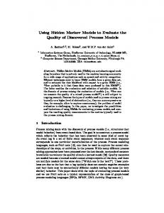
Fig. 1.
Structure of Matrix P
Fig. 2.
Structure of Matrix K
for every x ∈ R, where β = log(1/δ − 1). In fact, the log-likelihood ratio Li accepts a bound which is tighter than (15). Let the supremum of Li be x∗ , which is given in [3], and derived here for completeness. Since q� (x) is an increasing contraction mapping of x for every �, x∗ satisfies the following boundary condition q� (x∗ + β) = x∗ which gives " x∗ = log
eα (1 − e−β ) + 2
r
(50)
#
e2α (1 − e−β )2 + e−β . (51) 4
Thus, one can apply a quantizer with M levels to [−x∗ − β, x∗ + β], and denote the resulted sample sequence by x ˆ. Denote the M -sample sequence of F (·) evaluated on x ˆ by an M × 1 vector F . Since the right hand side of (49) is a linear combination of shifted versions of F (·), one can multiply F by a matrix K together with the help of an auxiliary constant vector d to obtain the discretized expression. The discretization of left hand side of (49) involves quantizing the logarithm, which is a contraction mapping from R to (−α, α). One can simply quantize the values of F (·) evaluated at q� (ˆ xi ), i = 1, · · · , M , where x ˆi is the ith element of x ˆ, to the nearest sample point in F . This can be done by pre-multiplying F by a scrambling matrix P . Thus, one can convert the non-linear fixed-point functional equation (49) to the following linear system PF = d + KF .
(52)
When a uniform quantizer is used, the matrices P and K have the structure depicted in Fig. 1 and Fig. 2 respectively. In Fig. 1, the elements on the curve are all 1’s and the rest of the elements in the matrix are 0’s. In Fig. 2, all elements on line (1) take the value (1 − �)(1 − δ), all elements on line (2) take the value (1 − �)δ, on line (3) take the value −�(1 − δ) and on line (4) take the value −�δ. The rest of the elements in the matrix are 0’s. There are many different ways for numerically solving the linear system (52), such as Gaussian elimination and QR factorization. Some are quite efficient if we utilize the sparsity of the matrices P and K. For ease of imposing the monotonicity of the cdf F , we choose to solve the following
quadratic programming with linear convex constraints. min k(K − P)F + dk2 F
(53)
s.t. Fi = 0, 1 ≤ i ≤ M1 ; Fi − Fi−1 ≥ 0, M1 + 1 ≤ i ≤ M1 + M2 + 1; Fi = 1, M 1 + M2 + 1 ≤ i ≤ M 1 + M 2 + M 3 , where Fi denotes the ith element of F , and M1 , M2 and M3 denote the number of samples in the intervals [−x∗ −β, −x∗ ), [−x∗ , x∗ ] and (x∗ , x∗ + β] respectively. Since the feasible region of the quadratic programming is a compact convex set, the optimal solution exists. The uniqueness of solution requires a detailed study on the matrix (K − P), which in general is difficult. Fortunately, since the cdf of Li conditioned on Xi−1 = +1 is unique, this quadratic programming does give a unique solution when the maximum sampling interval length is small. There are many methods for solving the quadratic programming problem (53), among which we use the active set method [13]. Although the number of iterations depends on the initial test value, this method can give a quadratic convergence rate [14], which makes the entire computation fast. Once the cdf F (·) is obtained, the entropy and input-output mutual information can be computed using either the direct method (see Section IV-A) or an information-estimation relationship (see Section IV-B). If the latter method is employed, one can utilize FFT and IFFT to compute the distribution of the left hand side of (48) conditioned on either Xi = −1 or Xi = +1, because the pdf of the sum of two independent random variables is the convolution of the pdf of each of the two random variables. As long as the distributions of log Λ conditioned respectively on Xi = −1 and Xi = +1 are obtained, one can average them with equal probability to obtain the distribution of log Λ. Fig. 3 gives the numerical results for BSC. The entropy rate of the output process is plotted as a function of � and δ. A uniform quantizer is used for computation.
B. Example 2: AWGN Channel For AWGN channel described by the following model √ Y = γX + N (54)
uniqueness of the solution to such a fixed-point functional equation are justified using the martingale theory and a contraction mapping property respectively. Although in general these equations cannot be solved analytically, numerical methods have been developed to give an effective approximation. The resulting distribution allows straightforward computation of the entropy rate of the hidden Markov process.
0.7
Entropy rate (nats)
0.6 0.5 0.4 0.3 0.2
R EFERENCES
0.1 0 0.5 0.4
0.5 0.3
0.4 ε
0.3
0.2
0.2
0.1
0.1 0
δ
0
Fig. 3. Entropy Rate of BSC with respect to the transition probability of the Markov chain � and that of the BSC δ.
where N ∼ N (0, 1), the conditional cdf F satisfies
Differential Entropy Rate (nats)
F (q� (x)) = � + E {(1 − �)F (x − 2W ) − �F (−x − 2W )} (55) √ for every x ∈ R, W ∼ N ( γ, 1). To linearize (55), one needs to also quantize the support of distribution of W . Because it is a standard Gaussian distribution, one can take samples on a finite interval, e.g. [−5, 5], and get a good approximation. In this case, the right hand side in linearized (55) will be expressed as the superposition of shifted versions of F (·) due to different quantization levels of W . The matrix K in (52) is dense in this case. Numerical results for AWGN channel with a uniform quantizer is illustrated in Fig. 4. The differential entropy rate is plotted as a function of the crossover probability � and the signal-to-noise ratio γ.
2.2 2 1.8 1.6 1.4 0.5 0.4
10
0.3 ε
8 6
0.2 0.1 0
Fig. 4.
2
4
γ
0
Differential Entropy Rate of AWGN Channel w.r.t. δ and γ.
VI. C ONCLUSION This paper derives fixed-point functional equations to characterize the stationary distribution of an input symbol from a binary symmetric Markov chain conditioned on the past observations under general channel models. The existence and
[1] D. Blackwell, “The entropy of functions of finite-state Markov chains,” in Trans. First Prague Conf. Information Theory, Statistical Decision Functions, Random Processes, pp. 13–20, (Prague, Czechoslovakia), House Chechoslovak Acad. Sci., 1957. [2] W. M. Wonham, “Some applications of stochastic differential equations to optimal nonlinear filtering,” SIAM J. Control Optim., vol. 2, pp. 347– 368, 1965. [3] E. Ordentlich and T. Weissman, “New bounds on the entropy rate of hidden Markov processes,” (San Antonio, Texas), pp. 117–122, Inf. Th. Workshop, October 24-29 2004. [4] C. Nair, E. Ordentlich, and T. Weissman, “Asymptotic filtering and entropy rate of a hidden Markov process in the rare transitions regime,” (Adelaide, Australia), pp. 1838–1842, Int. Symp. Inf. Th., Sep. 4-9 2005. [5] Y. Ephraim and N. Merhav, “Hidden Markov Processes,” in IEEE Trans. Information Theory, vol. 48, no. 6, June 2002. [6] H. Pfister, J. Soriaga, and P. Siegel, “On the achievable information rates of finite state ISI channels,” (San Antonio, TX), pp. 2992–2996, IEEE GLOBECOM, Nov. 2001. [7] D. Arnold and H. Leoliger, “The information rate of binary-input channels with memory,” (Helsinki, Finland), pp. 2692–2695, 2001 IEEE Int. Conf. Communications, Jun. 2001. [8] S. Egner, V. Balakirsky, L. Tolhuizen, S. Baggen, and H. Hollmann, “On the entropy rate of a hidden Markov model,” (Chicago, IL), p. 12, Int. Symp. Inf. Th., June-July 2004. [9] H. Pfister, “On the Capacity of Finite State Channels and the Analysis of Convolutional Accumulate-m Codes”, Ph.D thesis, pp. 148–151, 2003. [10] E. Ordentlich, and T. Weissman, “Approximations for the Entropy Rate of a Hidden Markov Process,” (Adelaide, Australia), Int. Symp. Inf. Th., Sep. 4-9 2005. [11] F. Jones, “Lebesgue Integration on Euclidean Space (Revised Edition),” Jones and Bartlett Publishers, 2001. [12] D. P. Palomar and S. Verd´u, “Representation of mutual information via input estimates,” in IEEE Trans. Information Theory, vol. 53, no. 2, Feb. 2007. [13] P. E. Gill, W. Murray, and M. H. Wright, Practical Optimization. Academic Press, 1981. [14] T. Coleman and Y. Li, “A reflective Newton method for minimizing a quadratic function subject to bounds on some of the variables,” SIAM J. Optim., vol. 6, no. 4, pp. 1040 – 1058, 1996. [15] K. B. Athreya and S. N. Lahiri, “Measure Theory and Probability Theory,” New York: Springer, 2006.