In this paper, we characterize the price equilibrium in a Hotelling model where firms face ... Bertrand-Edgeworth competition with differentiated products is the fact that product ... This is guaranteed to happen if a monopolist covers the market.
On the Nature of Equilibria when Bertrand meets Edgeworth on Hotelling’s Main Street∗ Nicolas Boccard† Xavier Wauthy‡ July 2009
Abstract In this paper, we characterize the price equilibrium in a Hotelling model where firms face capacity constraints. For a wide range of capacity levels, a pure strategy equilibrium does not exist. When this is the case, we show that in a mixed strategy equilibrium firms use a finite number of prices and the number of price in their support differ by at most one.
1
Introduction
Bertrand (1883)–Edgeworth (1925) competition has generated a considerable amount of research in recent years. Curiously enough, most of this research effort remained confined to the case of markets where firms sell homogeneous goods. Building on the initial results of Kreps and Scheinkman (1983), the strategic value of capacity limitation as a way to relax price competition has been tested in various context. Some important references in this respect are Benoˆıt and Krishna (1987), Davidson and Deneckere (1986), Deneckere and Kovenock (1992), Deneckere and Kovenock (2005) or Allen et al. (2000). By contrast, almost no progress has been made in the analysis of Bertrand-Edgeworth competition in markets with differentiated products. A possible explanation for the lack of interest in Bertrand-Edgeworth competition with differentiated products is the fact that product differentiation already relaxes competition, so that firms enjoy positive payoffs in equilibrium. The corresponding models therefore offer tractable setups in which to study multi-stage games with various forms of commitment, which populates the IO field. Indeed, equilibrium outcomes in the corresponding price subgames are “appealing“. A second reason which possibly explains the relative disinterest for this class of games is the fact that the standard techniques which are used to solve Bertrand–Edgeworth games with homogenoeus goods do not work at all in the case of differentiated products. Apart from very special cases (such as Krishna (1989), Furth and Kovenock (1993) or Boccard and Wauthy (2005)), very little is known about the structure of mixed strategy equilibria in such markets. The ∗ †
This paper is based on the CORE DP #9783 “Hotelling model with capacity pre-commitment“, 1997. Departament d’Economia, FCEE, Universitat de Girona, 17071 Girona, Spain. Financial support from Generalitat
de Catalunya (2005SGR213 and Xarxa de refer`encia d’R+D+I en Economia i Pol´ıtiques P´ ubliques) and Ministerio de Educaci´ on y Ciencia (SEJ2007-60671) are gratefully acknowledged. ‡ CEREC, Facult´es Saint-Louis Bruxelles and CORE, Universit´e Catholique de Louvain.
aim of the present paper is precisely to offer a detailed characterization of the structure of these equilibria in a particular, though quite standard, model, namely, the Hotelling (1929) model.1 More precisely, we shall analyze the structure of price equilibria in a pricing game where products are differentiated “` a la Hotelling” and firms face rigid capacity constraints. It is well-known that in such a model, there will exist no pure strategy equilibrium when capacities take intermediate values, relative to the differentiation parameters. This result, though already conjectured by Edgeworth, has been proved formally in various contexts (Canoy (1996), Furth and Kovenock (1993), Wauthy (1996), Benassy (1989)). Yet, product differentiation and smooth rationing guarantee demand continuity which then translate to payoffs so that the existence of a mixed strategy equilibrium is not an issue (by Glicksberg (1952)’s theorem). What is at stake is the structure of a mixed equilibrium for such cases. In this contribution we establish essentially three results: first, firms use atoms in equilibrium, i.e. the support of the equilibrium mixed strategy is finite. Second, we show that the number of atoms used by the firms differ by at most 1. Third, the number of atoms in the support of an equilibrium decreases with the relative degree of product differentiation. The present paper’s contribution is therefore mainly methodological. In particular we do not explicitely compute all the mixed strategy equilibria and do not characterize equilibrium payoffs. We are also silent on the uniqueness issue. All those issues are of course very relevant but we leave them to future research. Let us stress however that the methodology laid out in this paper is likely to be useful in addressing other economic problems characterized by continuous but non-concave payoffs. Typical examples are the class of switching-cost models with product differentiation (Klemperer (1987)) or duopoly models of price discrimination with differentiated products.
2
The model
2.1
Unconstrained Capacities
Two shops are located at the boundaries of the [0; 1] segment along which consumers are uniformly distributed. The indirect utility derived by a consumer indexed by x ∈ [0, 1] when buying product 1 or 2 is defined as v − x − p1 and v − (1 − x) − p2 respectively. Refraining from consuming any of the two products yields a nil level of utility. Consumers buy at most one unit of the product. As in most of the literature, we assume market coverage in equilibrium i.e., that firms do not wish to act as local monopolists. This is guaranteed to happen if a monopolist covers the market. The monopoly profit being p(v−p), the optimal price is v2 ; it thus attracts the most distant customer if v − 1 −
v 2
> 0 ⇔ v > 2.
The indifferent consumer, denoted x ˜(p1 , p2 ), solves v − x − p1 = v − (1 − x) − p2 i.e., x ˜(p1 , p2 ) = 1
1 − p1 + p2 2
(1)
While we were in the process of rewriting this paper, our attention has been attracted on Sinitsyn (2009) who
offers comparable characterizations in a different setup. While the basic games are very different, it is clear that the logic behind the characterizations are identical. Since the author does not mention any of our previous contributions in his paper, it seems fair to consider that his contributions and ours have been developed independently from each other.
2
The market is non-covered whenever v−x ˜(pi , pj ) − pi < 0 ⇔ pi + pj > 2v − 1
(2)
i.e., at prevailing prices, at least one consumer prefers to refrain from buying. In such a case, firm i is a local monopolist with demand Di = min {1, v − pi }. When firms name prices low enough, the market is covered so that demands are D1 = x ˜(p1 , p2 ) and D2 = 1 − x ˜(p1 , p2 ). Accordingly, the demand function of firm i is
Di (pi , pj )|pi ≤2v−1−pj
Di (pi , pj )|pi ≥2v−1−pj
=
0
if pi > pj + 1
1−pi +pj 2
if pj − 1 ≤ pi ≤ pj + 1 1 if pi < pj − 1 if pi > v 0 = v − pi if v − 1 ≤ pi ≤ v 1 if pi < v − 1
(3)
(4)
In this section, each firm is able to cover the entire market so that profit is π i (pi , pj ) = o n 1+pj , p − 1 along (3) or max{v − 1, 2v − 1 − pj } pi Di (pi , pj ). The best reply is either max j 2 o o n n 1+pj , p − 1 , v − 1 along (4) as v > 2 is assumed. The best reply is thus Φ(pj ) = min max j 2 The standard Hotelling equilibrium pi = pj = 1 covers the market. We analyze this game of complete information with the concept of Nash equilibrium. W.l.o.g. pure (price) strategies belong to the compact [0; v]. A mixed strategy is σ ∈ ∆, the space of (Borel) probability measures over [0; v], its support2 is Γ(σ), σ = inf(Γ(σ)) and σ = sup(Γ(σ)). The following result is well known but its proof includes unusual convexity considerations hinting at the results to come. Lemma 1 If min{k1 , k2 } ≥ 1, the equilibrium is uniquely defined by (1,1). Proof With ample capacities, sales equate demand. Since Di is piecewise linear and decreasing in pj , π i is strictly concave in pj whenever Di (pi , pj ) > 0. If positiveness was not an issue, we would be able to use the fact that the expectation of a strictly concave function is strictly concave to claim that the best response to a mixed strategy is a pure one because a strictly concave function has a unique maximum over a compact domain. As demand may become nil, the previous argument cannot be used. Yet, the knowledge of the best reply is useful to eliminate strictly dominated strategies. It is trivial to check that no firm wants to price above suppj Φ(pj ) = v − 1. Indeed, a lower price does better against any opponent’s price, thus against any mixed strategy of the opponent. Using this information for the other player means that no one wants to price above Φ(v − 1) < v − 1 (by construction of Φ). Reiterating, we see that no firm wants to price above the greatest fixed point of Φ. Likewise, no firm wants to price below inf pj Φ(pj ) = 21 . Hence, no firm wants to price below Φi ( 12 ) = 43 . By the same token, no firm wants to price below the smallest fixed point of Φ. Since Φ has a unique fixed point at 1, uniqueness of the equilibrium is proved. � 2
Set of all points for which every open neighbourhood has positive measure.
3
2.2
Constrained Capacities
We now consider a pricing game G(k1 , k2 ) where (k1 , k2 ) denote the capacity levels that firms are committed to. Firms cannot produce beyond capacities and thus ration consumers whenever demand exceeds capacity.3 In order to analyse the pricing game, we must therefore specify the organisation of the rationing. We follows Kreps and Scheinkman (1983) in assuming that the efficient rationing rule is at work in the market. Under this rule, rationed consumers are those exhibiting the lowest net reservation price for the good. In the example depicted on Figure 1, all consumers located in [0, x ˜(p1 , p2 )] want to buy at firm 1 but some will be rationed. Under efficient rationing, those rationed consumers are located in [k1 , x ˜(p1 , p2 )]. Note that they are precisely the most inclined to switch to firm 2 since they exhibit the largest net reservation price for product 2 within the set [0, x ˜(p1 , p2 )] .
Potential demand Potential demand for firm 1 for firm 2 $� %� &� $� %� &� x �� � 1 k1 0 x (p 1, p 2 ) "� "� �!� �� "� "� �!��� �� Sales of firm 1�� Sales of firm 2 �� "� "� � !� Rationed consumers switching �� from firm 1 to firm 2 Figure 1: Demand vs. Sales Extreme capacities, analyzed in Lemmas 1 and 7 (in the appendix), lead to the conclusion that firms have incentives to set intermediate values. Our focus is thus on the situation where each firm is unable to serve the entire market by herself but the industry can i.e., k2 ≤ k1 < 1 and k1 + k2 ≥ 1 (which implies k1 ≥ 12 ).
3
Equilibrium analysis
3.1
Rationing
The original Hotelling analysis must be amended to account for binding capacities and rationing. Referring to equations (3–4), we may identify two different ways through which firm i’s demand, and therefore payoffs can be affected. For high prices (first segment), a firm may enjoy a positive demand if it captures part of the consumers rationed by firm j. More generally, in the domain where the market is covered, her demand may be strictly positive even for high price differentials. On the other hand, its sales are bounded from above by the installed capacity. To derive sales, we must first delineate the areas where firms are constrained. According to the analysis developed when building equations (3) and (4), we already know that the price space must be partitioned according to market coverage. The solution in p1 to equation (2) is c(p2 ) = 2v − 1 − p2 3
The firm will refuse to produce beyond “capacity” if the marginal cost jumps beyond S.
4
(5)
We must also identify the constellations of prices for which capacity constraints are binding. D1 (p1 , p2 ) = k1 ⇒ p1 = a(k1 , p2 ) ≡ p2 + 1 − 2k1
(6)
D2 (p1 , p2 ) = k2 ⇒ p1 = b(k2 , p2 ) ≡ p2 − 1 + 2k2
(7)
Hence, firm 1 is capacity constrained if p1 ≤ a(k1 , p2 ), no firm is capacity constrained if a(k1 , p2 ) ≤ p1 ≤ b(k2 , p2 ) and firm 2 is capacity constrained if b(k2 , p2 ) ≤ p1 . To connect areas, we solve: c(p2 ) = a(k1 , p2 ) ⇒ p2 = ρ(k1 ) ≡ v + k1 − 1
(8)
c(p2 ) = b(k2 , p2 ) ⇒ p2 = δ(k2 ) ≡ v − k2
(9)
Next, observe that δ(k1 ) = a (k1 , ρ(k1 )) and ρ(k2 ) = b (k2 , δ(k2 )). This means that the pair (ρ(k2 ), δ(k2 )) defines the highest prices such that firm 2 is exactly selling its capacity while firm 1 sells the market complement. A symmetric conclusion holds for (δ(k1 ), ρ(k1 )). In the region where the market is covered and firm 1 is capacity constrained (a(.) ≥ p1 ), firm 2 sells 1 − k1 as long as p2 ≤ ρ(k1 ). The residual demand addressed to firm 2 is 1 − k1 in this region and is therefore locally independent of prices. Figure 2 illustrates our findings.
p1 D1 = v − p1 D2 = k2
ρ(k2)
D1 = 1 − k2 D2 = k2
D1 = v − p1 D2 = v − p2
c
δ(k1)
b
a
D1 = 1 − x D2 = x
D1 = k1 D2 = 1− k1 δ(k2)
D1 = k1 D2 = v − p2
ρ(k1)
p2 2v - 1
Figure 2: The Sales Space Notice that k1 + k2 > 1 implies a(.) < b(.) and δ(kj ) ≤ ρ(ki ). The non void area delimited by the − functions a(.), b(.) and c(.) is referred to as “the band”. We define p− 1 = b(0, k2 ) and p2 = 2k1 −1 ≤ 1,
the solution to a(p2 , k1 ) = 0 (k1 ≥
1 2
implies a(k2 , 0) ≤ 0).
Then the sales function of firm 1 can be defined as ˜(p1 , p2 ) x if p2 ≤ p− 2 , S1 (p1 , p2 ) = 1 − k2 v−p 1
5
follows: if 0 ≤ p1 ≤ b(p2 , k2 ) if b(p2 , k2 ) ≤ p1 ≤ ρ(k2 ) if ρ(k2 ) ≤ p1 ≤ v
(10)
k1 x ˜(p1 , p2 ) if p− ≤ p ≤ δ (k ), S (p , p ) = 2 2 2 1 1 2 2 1 − k2 v − p1
if δ 2 (k2 ) ≤ p2 ≤ ρ(k1 ), S1 (p1 , p2 ) =
if ρ(k1 ) ≤ p2 , S1 (p1 , p2 ) =
if 0 ≤ p1 ≤ a(p2 , k1 ) if a(p2 , k1 ) ≤ p1 ≤ b(p2 , k2 ) if b(p2 , k2 ) ≤ p1 ≤ ρ(k2 )
(11)
if ρ(k2 ) ≤ p1 ≤ v
k1
if 0 ≤ p1 ≤ a(p2 , k1 )
x ˜(p1 , p2 ) if a(p2 , k1 ) ≤ p1 ≤ c(p2 ) v−p if c(p2 ) ≤ p1 ≤ v 1 ( k1 if 0 ≤ p1 ≤ δ(k1 ) v − p1 if p1 ≤ (k1 )δ
(12)
(13)
The sales function S2 (p1 , p2 ) is entirely symmetric. Notice that sales are continuous and exhibit at most two constant segments corresponding to market shares ki and 1 − kj . Glicksberg (1952) then ensures the existence of a Nah equilibrium.
3.2
Equilibrium Analysis
Having obtained the firms’ sales function, we now characterize firms’ best reply (BR) functions and identify Nash equilibria in G(k1 , k2 ). Given p2 , we seek the local incentives for firm 1 with the help of on Figure 2. Since v > 2, we have
v 2
< δ(k1 ) = v − 1 + k1 , hence the ideal monopoly price is below the line
“ρ(k2 )–c(.)–δ(k1 )” which means that the BR is at or below this line. Observe now that firm 1’s demand is constant below the line “a(.)–δ(k1 )”, hence the BR against p2 ≥ ρ(k1 ) is simply δ(k1 ). Below a(.), demand is constant, hence the optimal price is a(.) itself and since it also belongs to the band, the BR is that of the band. The candidate in the band being H1 (p2 ) =
1+p2 2 ,
the BR inside
the band is Φ1 (p2 ) = min {b(k2 , p2 ), max {H1 (p2 ), a(k1 , p2 )}}. Above b(.), demand is constant, hence the optimal price is ρ(k2 ) which we may call a “security price” as it ensures the “minmax” payoff π si ≡ ρ(kj )(1 − kj ). The cut-off price of firm 2 for which firm 1 is indifferent between Φ1 (p2 ) and ρ(k2 ) is γ(k1 , k2 ) such that π s1 = π 1 (Φ1 (p2 ), p2 ). In Lemma 6 of the Appendix, we show uniqueness and derive the explicit form of γ(k1 , k2 ) as well as the conditions under which it is positive. Letting α(k2 ) be defined as the solution to a(k1 , p2 ) =
1+p2 2 ,
we obtain α(k1 ) = 4k1 − 1. Firm i’s best reply correspondence, illustrated on Figure 3, is thus if pj ≤ γ(ki , kj ) ρi (kj ) 1+pj BRi (pj ) = if γ(ki , kj ) ≤ pj ≤ α(ki ) 2 p + 1 − 2k if max{α(k ), γ(k , k )} ≤ p j
i
i
i
j
(14)
j
The iterated elimination of dominated strategies along the lines of the proof of Lemma 1 leads to: h n o i πs Lemma 2 Γ(σ i ) ⊂ max 1, kii ; ρi (kj ) . Proof We proceed in several steps. i) To show σ i ≤ ρi (kj ), observe that ∀pj ≥ 0, ∀pi ≥ ρi (kj ), Si (pi , pj ) = v − pi , thus the average
6
p1 ρ(k2) δ(k1) q1 γ(k2,k1) 1 2 δ(k2) 12
p2
q2 γ(k1,k2) α(k1) ρ(k1)
Figure 3: Demand vs. Sales π i (σ j , .) is the monopoly payoff over that domain and it is strictly decreasing because the monopoly price
v 2
is less than ρi (kj ).
ii) Observe from (14), that BRi is either strictly increasing or greater than unity and in any case BRi ≥ Hi holds true. We may thus apply the proof of Lemma 1 to derive σ i ≥ 1. iii) The equilibrium payoff is larger than any deviation, hence π ∗i ≥ π i (σ j , ρi (kj )) = π si . Together with the fact that Si ≤ ki , we deduce σ i ≥
π si ki .
�
Proposition 1 There exist only three possible type of equilibria: i) Both firms quote the pure strategy Hotelling price. ii) One firm plays a mixed strategy displaying n + 1 atoms while the other plays a mixed strategy displaying n atoms, with n ≥ 1. iii) Both firms use a mixed strategy involving the same number of atoms. Proof Whenever γ 1 (k1 , k2 ) ≤ 1 and γ 2 (k1 , k2 ) ≤ 1, the best reply curves intersect at (1, 1) meaning that the pure strategy price equilibrium √ (1, 1) exists. Lemma 6 in the appendix proves that the h i 2−v+ v 2 −1/2 √1 , 1 . The rest of the proof derives from 3 condition reduces to min{k1 , k2 } ≥ ∈ 2 2 lemmas. 1. The support of a mixed strategy equilibrium distribution is finite. 2. The Hotelling equilibrium exists under sufficiently large capacities (case i)). 3. Existence of an equilibrium where one firm uses a pure strategy while the other mixes over two atoms. This equilibrium exists for intermediate capacities (case ii)). 4. Existence of (n, n + 1) and (n + 1, n + 1) equilibria, with ∞ > n ≥ 1 (case ii) continued and case iii) ). Let β 1 (k2 ) = 3 − 4k2 be the solution to b(k2 , p2 ) = identify β 2 (k1 ) as the level of p1 such that a−1 (k1 , p1 ) that
b−1 (k1 , p1 )
=
1+p1 2 .
7
1+p2 2 . A similar argument can be 1 = 1+p and α2 (k1 ) as the level of 2
used to p1 such
Lemma 3 The support of a mixed strategy equilibrium is finite. Proof Using the fact that Γ(σ i ) ⊂ [1; ρi (kj )], we define p01 = p02 = 1 and for m ≥ 1 let pm 1 = m m b(pm−1 , k2 ) and define pm 2 such that p1 = a(p2 , k1 ). Because industry capacity covers the market, 2
those sequences are strictly increasing thus reach the upper bounds for a finite m. Let p1 vary in [p01 ; p11 ]. Observe that ∀p2 ≥ p02 , D1 is decreasing concave (constant and then linear decreasing), thus so is π 1 . Since integration preserves this property, π 1 (., σ 2 ) has a unique maximum p1 over [p01 ; p11 ] which is the unique price on which firm #1 may put mass in equilibrium. Let p2 vary in [p02 ; p12 ]. Conditional on p1 > p11 , D2 is decreasing concave, thus so is π 2 . The Rv partial average y2 (p2 ) = p1 π 2 (p2 , x)dσ 1 (x) has then a unique maximizer. Now, there is α1 ≥ 0 such 1
that π 2 (., σ 1 ) = α1 π 2 (p2 , p1 ) + (1 − α1 )y2 (p2 ). Being the average of two locally concave functions, each with a unique maximizer, this payoff function has at most 2 maximizers over [p02 ; p12 ]. This shows that firm #2 uses at most 2 atoms over this interval. ∀ ∈ [p11 ; p21 ], ∀p2 > p12 , D1 is decreasing concave meaning that the partial average y1 (p1 ) = Rv
p12
π 1 (p1 , x)dσ 2 (x) has then a unique maximizer. Since firm #2 uses at most 2 atoms over prices
below p12 , π 1 (., σ 2 ) has at most 3 maximizers over [p11 ; p21 ]. Repeating the argument for each player alternatively adds a single potential atom at each step and since all prices are bounded, the supports of an equilibrium distribution must be finite. � Lemma 4 There exist mixed strategy equilibria where one firm uses a mixed strategy involving two atoms while the other uses a pure strategy4 . Proof The proof is by construction. Firm 2 plays γ 2 (k1 , k2 ) while firm 1 mixes (ν, 1 − ν) over ρ1 (k2 ) and p1 = Φ1 (γ 2 ). The pure strategy of firm 2 guarantees that firm 1 is indifferent between her two atoms. If the point (p1 , γ 2 ) belongs to the border of the band then firm 2 has a constant demand for p2 > γ 2 against ρ1 (k2 ) and p1 , thus a clear incentive to raise her price. The candidate equilibrium thus requires this point to be interior to the band i.e., p1 =
1+γ 2 (k1 ,k2 ) , 2
the Hotelling branch of the
best reply function (14). The condition on the parameters is γ 2 < α(k1 ) i.e., k1 large relative to k2 . We now need to find weights that make γ 2 (k1 , k2 ) a BR for Firm 2. We have � � 1 − p2 + p1 π 2 (ν, p2 ) = νp2 k2 + (1 − ν)p2 (15) 2 ∂π 2 (.) The FOC ∂p2 = 0 yields a solution ν ∗ since the first term is positive while the p2 =γ 2 (k1 ,k2 )
second is negative as γ 2 (k1 , k2 ) < 1. � Since we put no upper limit to v, the above condition will be violated for v large enough, thereby destroying our semi-mixed equilibrium. This is why we have to consider alternative candidate ni 5 equlibria, involving both firms using mixed strategies. Let (pm i )m=1 denote the (ordered) support s s≤n2 of an equilibrium strategy σ i . Given the matrix of price pairs (pm 1 , p2 )m≤n1 , we speak of a “line”
when for a fixed p1 and of a “column” for a fixed p2 . Last, the ”diagonal” is defined as the pairs m (pm 1 , p2 )m≥1 . 4
To the best of our knowledge, Krishna (1989) is the first paper identifying this particular type of equilibrium
under Bertrand-Edgeworth competition. 5 The “m” index bears to relation to that employed in Lemma 3.
8
Since the existence of an equilibrium is ensured by the continuity of payoff functions, if neither pure nor semi-mixed equilibria exist, then there exists an equilibrium in which both firms use nondegenerate mixed strategies. We furthermore know that firms use only atoms in an equilibrium. The intuititon underlying the proof rest on the piecewise concavity of payoffs and on the fact that within the band, there can be only one best reply. Starting from the pair of minimal atoms, we identify some restrictions on the distribution of the other atoms; these restrictions allow us to show that the cases where firms use the same number of atoms or the case where the large capacity firm puts n+1 atoms while the other names n prices are the only possible cases that satisfy the necessary conditions for a mixed strategy equilibrium. Lemma 5 There exist completely mixed strategy equilibria where either n1 = n2 or n1 = n2 + 1. Proof We prove that the number of atoms used by firms differ by at most one and ∀m ≤ n − 1, m we have 1 − 2k2 < pm 1 − p2 < 2k1 − 1. Observe firstly, as a by-product of Lemma 3, that ∀pi ∈
Γ(σ i ), ∃!pj ∈ Γ(σ j ) such that (pi , pj ) belong to the band; this is so because the profit in the band is strictly concave and has at most one maximizer (cf. y2 function in the proof). We use five successive claims with the help of Figure 4.
p1 p1
β
χ
α
ω
δ
ε
D2 = k2
p1
D1 = k1
p2
p2
p2 Figure 4: Atoms
1. The pair of minimal atoms (p11 , p12 ) lies in the band. If the minimal point was ω, not α, then firm #1 has a constant demand, thus would like to raise her price until ω hits the band. Likewise if the minimal point is β, firm #2 would like to raise her price until β hits the band. Define now α = (p11 , p12 ), ω = (p11 , p22 ), β = (p21 , p12 ). 2. ω and β lie strictly outside the band. Point ω cannot belong to the band, for otherwise α would not be the unique maximizer of π 2 over [0, k1 ), b(p1 , k2 )] (recall that π 2 is concave over that domain given that #1 plays at or above p1 ). The same applies for β wrt. profit maximization of firm #1. 3. The pair of minimal atom is strictly interior to the band. If α lies on the right border of the band, then firm #2 has constant demand at p12 because the 9
atoms of firm #1 are either above or below the band but not in. Price p12 is then not a best reply to σ 1 . The same applies for the upper side of the band. m 4. All points (pm 1 , p2 )m≤n−1 are strictly interior to the band.
The second “diagonal” point (p21 , p22 ) could be either χ, δ or ε as shown on Figure A1. If χ, then the ω − χ column would have no point in the band and π 2 (σ 1 , .) would be locally increasing at p22 . Likewise, if ε, the β − � line would have no point in the band. Hence, (p21 , p22 ) = δ. We m have thus shown that for m ≥ 1, (pm 1 , p2 ) lies in the band. Furthermore, the previous claim
implies that the point is strictly interior if m < min{n1 , n2 }. Only the last diagonal point could lie on one frontier of the band. 5. The number of atoms of equilibrium distributions differ by at most one. Suppose n1 = n, n2 = n + 1. We first show using argument similar to above that the last diagonal point must be interior to the band. Then the last point has to belong to the small upper triangle for it the only way to generate an interior maximum of the profit function. The case for n2 > n + 1 is now easy because π 2 (σ 1,. ) must have the same shape over [pn2 , pn+1 ] or 2 over [pn+1 , pn+2 ] leading to a contradiction. 2 2 � Notice that, when establishing step 1 in the above proof, we have relied on the fact that the iteration process would reach its end when we reach the finite upper bound of the equilibrium support. At the same time, it appears form this proof that the number of possible iteration, i.e. the number of successive atioms, is actually depending on the width of the band, relative to the value of ρ(ki ). Recalling that we have normalized the transportation cost to 1, v is sufficient to capture the relative importance of product differentiation into the model. An increase in v can be interpreted as a relative decrease in the degree of product differentiation. As a result an immediate by-product of the above argument is that the number of possible atoms in a mixed strategy equilibrium is inversly related to the magnitude of v. The less relevant is the differentiation dimension, the more numerous atoms are to be played in equilibrium.
4
Final Remarks
In this note, we have partially characterised the structure of mixed strategy equilibria in a Hotelling model where firms face capacity constraints. Our main results can be summarized as follows: in this setup, firms use a finite number of prices in equilibrium and the number of atoms they retain in equilibrium differ by at most one. This result is obviously a partial one and several extensions are called for. First, we do not fully characterize these equilibria. Second, we do not characterize, even partially, equilibrium payoffs. Third, we do not discuss uniqueness. These three problemsn should be addressed in order to allow for the analysis of capacity commitment games. This is to a large extent a matter of computations. Relying on preliminary results, we offer the following conjecture: despite of the multiplicity of equilibria (which is is endemic is this class of models), there always exists an equilibrium in which the large capacity firm is held down to its minmax payoff.
10
Appendix Lemma 6 The cut-off price γ(k1 , k2 ) is defined as follows o n p max 0, 8(v − 1 + k2 )(1 − k2 ) − 1 if k2 ≥ γ(k1 , k2 ) = (v−1+k2 )(1−k2 ) − 1 + 2k1 if k2 ≤ k1
√
v 2 −8k12 2 √ 2−v+ v 2 −8k12 2
2−v+
(16)
Proof The best reply of firm 1 within the band is either H1 (p2 ) or a(k1 , p2 ) depending on whether she hits her capacity or not. We have D1 (H1 (p2 ), p2 ) < k1 ⇔ p2 ≤ 4k1 − 1. Accordingly, the payoff accruing to firm 1 when she plays her best reply within the band is ( 2 2) if p2 ≤ 4k1 − 1 π 1 (p2 ) = (1+p 8 π 1 (p2 ) = π 1 (p2 ) = k1 (p2 + 1 − k2 ) if p2 ≥ 4k1 − 1
(17)
These payoffs are then to be compared to those accruing from the security strategy ρ1 (k2 ), i.e. p π s1 (k2 ) = (v − 1 + k2 )(1 − k2 ). The solution to π s1 (k2 ) = π 1 (p2 ) is p2 = 8(v − 1 + k2 )(1 − k2 ) − 1 while that of π s1 (k2 ) = π 1 (p2 ) is p2 = (v−1+kk21)(1−k2 ) − 1 + 2k1 . Observe that if v is too small, p p 8(v − 1 + k2 )(1 − k2 )−1 is negative and the security strategy is never used; also 8(v − 1 + k2 )(1 − k2 )− 1 gives us a bound when considering large values of k2 as π s1 (k2 ) is decreasing. Taking care of the negative solution, we have p 1 8(v − 1 + k2 )(1 − k2 ) − 1 ≤ 4k1 − 1 ⇔ k2 ≥ Φ(k1 ) ≡ 2
� � q 2 2 − v + v 2 − 8k1
(18)
This separates cases where the security strategy beats the standard Hotelling best reply (π 1 (p2 )) throught the whole relevant range from the alternative case. Hotelling Equilibrium
The necessary conditions are γ 1 (k1 , k2 ) < 1 and γ 2 (k1 , k2 ) < 1. Observe
from (6) that γ 1 (k1 , k2 ) < 1 ⇔ ( k2 ≤ Φ(k1 ) (v−1+k2 )(1−k2 ) k1
− 1 + 2k1 < 1
)
( or
2−v+
√
k2 ≥ Φ(k1 ) p 8(v − 1 + k2 )(1 − k2 ) − 1 < 1
)
v 2 −8k (1−k )
1 1 In the first case, the condition yield k2 > . In the remaining case, the condition 2 √ 2 h i 2−v+ v −1/2 is k2 > Φ(1/2) = ∈ √12 , 1 (as v > 2). By symmetry for k1 , the Hotelling equilibrium 2
exists for capacities greater than Φ(1/2) (drawing the two curves shows that). � Lemma 7 If k1 + k2 < 1, there is a unique equilibrium; it is in pure strategies. Proof When aggregate capacities are smaller than the market size (k1 + k2 < 1), firms do not compete at all since their potential market shares cannot overlap. In this “local monopoly” case, denoted GL (k1 , k2 ), firms sell either at the monopoly price or at full capacity if the WTP is large enough. In any case, they have maximal incentives to increase capacities. Demand is Di = min {v − pi ; ki } and profit is π i = pi min {v − pi ; ki } which is maximum for � pi = max v − ki ; v2 . Thus whenever 1 − kj > ki ≥ v2 , firm i acts as a pure monopolist whereas in the complementary case, she sells her capacity at the price pki = v − ki which makes consumer located at a distance ki indifferent between buying product i or refraining from consuming. � 11
References Allen B., Deneckere R., Faith T., and Kovenock D. Capacity precommitment as a barrier to entry, a bertrand-edgeworth analysis. Economic Theory, 15:501–530, 2000. Benassy J. P. Market size and substitutability in imperfect competition: a bertrand-edgeworthchamberlain model. Review of Economic Studies, 56:217–234, 1989. Benoˆıt J.-P. and Krishna V. Dynamic duopoly: Price and quantities. Review of Economic Studies, 44:23–35, 1987. Bertrand J. Th´eorie des richesses: revue de th´eories math´ematiques de la richesse sociale par l´eon walras et recherches sur les principes math´ematiques de la th´eorie des richesses par augustin cournot. Journal des Savants, 67:499–508, 1883. Boccard N. and Wauthy X. Equilibrium payoffs in a bertrand-edgeworth model with product differentiation. Economics Bulletinulletin, 12(11), 2005. Canoy M. Product differentiation in a bertrand-edgeworth duopoly. Journal of Economic Theory, 1996. Davidson C. and Deneckere R. Long-run competition in capacity, short-run competition in price and the cournot model. RAND Journal of Economics, 17(3):404–415, 1986. Deneckere R. and Kovenock D. Price leadership. Review of Economic Studies, 59:143–162, 1992. Deneckere R. and Kovenock D. Bertrand-edgeworth duopoly with unit cost asymmetry. Economic Theory, 86:1–25, 2005. Edgeworth F. Papers relating to political economy, vol. 1, chapter The Theory of Pure Monopoly. MacMillan, New York, 1925. Furth D. and Kovenock D. Price leadership in a duopoly with capacity constraints and product differentiation. Journal of Economics, 57(1):1–35, 1993. Glicksberg I. L. A further generalization of the kakutani fixed point theorem, with application to nash equilibrium points. Proceedings of the American Mathematical Society, 3(1):170–174, 1952. Hotelling H. Stability in competition. Economic Journal, 39(153):41–57, 1929. Kreps D. and Scheinkman J. Quantity precommitment and bertrand competition yields cournot outcomes. Bell Journal of Economics, (14):326–337, 1983. Krishna K. Trade restrictions as facilitating practices. Journal of International Economics, 26(3-4): 251–270, 1989. Sinitsyn M. Price dispersion in duopolies with heterogeneous consumers. International Journal of Industrial Organization, 27(2):197–205, 2009. Wauthy X. Capacity constraints may restore the existence of an equilibrium in the hotelling model,. Journal of Economics, 64:315–324, 1996. 12