For ASR the source is not relevant, because it has different qualities for .... Beatles: 20 rock and pop songs (1.1h), interpreted by a string quartet. Soft Jazz - Sexy ...
ON THE REDUCTION OF FALSE POSITIVES IN SINGING VOICE DETECTION Bernhard Lehner, Gerhard Widmer, Reinhard Sonnleitner Department of Computational Perception Johannes Kepler University of Linz {bernhard.lehner,gerhard.widmer,reinhard.sonnleitner}@jku.at
ABSTRACT Motivated by the observation that one of the biggest problems in automatic singing voice detection is the confusion of vocals with other pitch-continuous and pitch-varying instruments, we propose a set of three new audio features designed to reduce the amount of false vocal detections. This is borne out in comparative experiments with three different musical corpora. The resulting singing voice detector appears to be at least on par with more complex state-of-the-art methods. New features and classifier are very light-weight and in principle suitable for on-line use. 1. INTRODUCTION There has been quite some research on the problem of automatic detection of a singing voice in audio recordings, and various more or less complex methods have been proposed. In particular, the method of Mauch et al. [1] seems to yield very good results — perhaps the best achieved so far — but with a rather complicated and expensive set of features (based, e.g., on the f0 trajectory of the predominant source). In a recent paper [2], we have shown that with a very simple and lightweight feature set (essentially, only appropriately selected and optimised MFCCs), we can achieve recognition results that are almost on par with such more complicated methods, and thus that the ‘baseline’ in this field should probably be placed higher than has been assumed so far. Our experiments also showed that the problem is not so much recall (i.e., the correct recognition of singing voice when there is a singing voice present), but precision: we encountered many false positives, caused in many cases by the presence in the signal of other pitch-continuous and pitchvarying instruments (e.g., violins, electric guitars etc.). In this paper, we introduce three new audio features – the Fluctogram – a representation of characteristic pitch fluctuations; the Spectral Contraction (SC) – an indicator of reliability of information in a given frequency band; and the Vocal Variance (VV) – a measure of variance in a specific subset of MFCC coefficients. These features, together with common MFCCs, permit us to build a singing voice detector (using a random forest classifier) that substantially ameliorates the above-mentioned false positive problem.
Two sets of experiments will be presented. The first set, based on rather specialised music collections, is intended to verify the hypothesis that the new features indeed alleviate the false-positive (voice-instrument mixup) problem. The second set of experiments, performed on standard benchmark corpora used in the singing voice detection literature, will show that the new method also produces improvements on general realworld music collections (though of course not as spectacular as with our worst case scenarios). As in [2], this is an extremely light-weight set of features that would be suitable for an on-line voice detection algorithm (minus the latency introduced by the observation windows used in the computation of the Fluctogram and the VV). 2. FEATURES FOR SINGING VOICE DETECTION In order to be able to distinguish highly harmonic instruments from singing voice, simply adding more static features like harmonic coefficient is not helpful [3]. Therefore, we suggest a set of features that describe temporal characteristics of the signal. Moreover, we do not rely on the premise that vocals are the predominant source in the mix, nor do we estimate an actual pitch, as do Mauch et al. in [1] or Ramona et al. in [4]. 2.1. Fluctogram The Fluctogram is basically an extension of a feature suggested by Sonnleitner et al. [5] for speech detection in mixed audio signals. The basic idea behind their feature is to detect sub-semitone fluctuations of partials by using the cross correlation. Each spectrum of a time frame Xt is compared to the subsequent one Xtt+1 , and the index of the maximum correlation when Xtt+1 is shifted ±n bins, is calculated. To make this concept more suited to our problem, we extend it by calculating these maximum correlation shift indices separately for different frequency bands. We first compute the magnitude spectrum by performing a DFT on audio frames of length 100ms, with a hop size of 20ms, and applying a zero padding of 23 . We then map the spectrum to a scale that relates to pitch, where 10 bins is the range of one semitone. This is necessary since fluctuating trajectories of the partials need to be equidistant for the cross correlation to reveal them.
NP −1
sc[n] =
Xn2 [j]win
j=0 NP −1
(1) Xn2 [j]
j=0
Fig. 1. A Spectrogram and the corresponding Fluctogram. Our pitch scale comprises six octaves from E3 (164 Hz) to E9 (10548 Hz). Finally, we divide our scaled spectrum into 17 bands, with each band 240 bins wide, which equals a bandwidth of two octaves. The distance from one band to the next is 30 bins, which equals three semitones. Each band is then weighted by a triangle window that matches the bandwidth. The harmonic fluctuations within each band are quantified with the aforementioned method by using the cross correlation and looking at shifts of ±5 bins, which equals half a semitone. Hence, only sub-semitone, pitch-continuous fluctuations are targeted and detected, as can be seen in Fig. 1. As a last step, we characterise each frame of audio by calculating the variance over a window of 40 successive Fluctogram values, centered on the current frame, separately for each band. This results in 17 values per audio frame, which we use as our Fluctogram feature. 2.2. Spectral Flatness and Spectral Contraction Since the Fluctogram is error-prone under certain circumstances, we need additional information that relates to the reliability of its values in the individual bands. The Fluctogram is most reliable when the signal is not noise-like, and most of the energy is concentrated near the center. As an estimation of the noise we use the Spectral Flatness (SF) measure [6], and we characterise an audio frame by the means of the flatness values over a window of 40 frames, for each frequency band, yielding another 17 feature values. The second feature, which we call Spectral Contraction (SC), was inspired by Spectral Dispersion [7], which also measures how much of the energy in the spectrum resides in the center, but has a few shortcomings. Our SC feature is basically the ratio of a weighted spectrum to the spectrum Xn [j] itself as given in Equation 1. By choosing a proper weighting window win, we allow the ratio to be relatively stable, even when there are sub-semitone fluctuations near the center. Therefore, we use a Chebyshev window with a sidelobe attenuation of 200db. The result is normalised in the range [0 − 1], where small values indicate the energy is widely dispersed. Large values indicate that the energy is primarily concentrated near the center.
To relate the Spectral Contraction to the Fluctogram, its variance over 40 successive frames is computed for each band, which gives another 17 feature values. Unfortunately, the features suggested so far have only limited discriminative power when highly harmonic, pitchcontinuous instruments like guitars, strings, flutes, are the predominant source. Therefore, we need an additional feature to describe a characteristic that is common only in singing voice: articulating actual words. Although some instruments are capable to articulate vowel-like sounds (e.g. guitars with wah-wah effect), their range is limited, i.e. it is impossible to articulate actual words with those instruments. 2.3. Vocal Variance For the task of automatic speech recognition (ASR), MFCCs are the most utilised features because of their close relationship to the source-filter model. According to this model, speech can be considered the result of the convolution of a source (i.e. the vocal chords), and a filter (i.e. the vocal tract). For ASR the source is not relevant, because it has different qualities for different speakers, and the filter is the most important parameter, since it is mostly independent from the speaker. Due to the application of a discrete cosine transform (DCT) as a last step of calculating MFCCs, the first few coefficients represent the slow variations of the spectrum that are related to changes of the shape of the vocal tract [8]. Therefore we suggest a novel feature, called the Vocal Variance (VV), which is supposed to reveal such variations. The VV comprises 5 values, computed on the first five MFCCs only (excluding the 0th). For each of these 5 first coefficients, we compute its variance over 11 successive frames centered on the current frame. To illustrate the usefulness of the VV, we compare a piece of a song with a high false positive rate (from the String Quartet testset) to a piece of a vocal only song in Figure 2. Clearly, the first five coefficients show differences between the instruments and vocals, but the higher frequency coefficients 21-25 do not share this discriminative power. 2.4. Complete Feature Set and Final Classifier For singing voice detection, the audio signal is analysed and classified with a time resolution of 200ms. That is, we have 5 training examples per second, each characterised by 116 features computed around the current time point: 17 Fluctogram variance features, 17 Spectral Flatness means and 17 Spectral Contraction variances, 60 MFCC features (30 MFCCs plus corresponding deltas), and 5 Vocal Variance features.
acc [%] recall precision f-measure
Fig. 2. Comparison of the discriminative power of lower and higher frequency MFCCs. As can be seen, only the first 5 coefficients show differences between instruments and vocals. We use the Random Forest algorithm [9] implemented in the machine learning framework WEKA [10] to learn a binary classifier that decides, for a given audio window, whether that window contains a singing voice or not. The classifier’s predictions are then smoothed over the sequence of windows using a median filter in two passes. We first smooth the continuous classifier output (classification probabilities) with a median filter of order 4 (800ms), then use a median filter of order 5 (1.0s) as a majority voter. 3. EXPERIMENTS We present three experiments. First, we train our classifier on an internal data set, and in the process compare it to a method from the literature that we were able to re-implement. This classifier is then used unchanged in the next two experiments. In experiment 2, we specifically investigate the ability of the new features to alleviate the problem with false positives and the voice-instrument mixup problem. For that, we select four music collections that contain no singing voice whatsoever, but instead have different instruments as dominant melody instrument. Finally, we compare our new classifier to two stateof-the-art methods for which experimental procedure and results are available from the literature and for which we have the corresponding datasets. The experiments will show that our new features also help in more general musical settings. 3.1. Training and Evaluating the Classifier For building our classifier and doing a first evaluation, we used an internal music collection of 75 annotated songs by 75 different artists. All songs were downsampled to 22kHz and converted to mono. Approximately 52% of the frames are annotated as vocal, and the amount of pure singing, i.e. without instrumental accompaniment, is negligible. We compare our classifier to what we consider the new baseline in the field: our simple MFCC-based classifier from [2]. We also include a comparison with the method by Vembu & Baumann (VB), which is described in [11] in such detail (including all the parameters) that we could confidently reimplement it. VB use 13 MFCCs, 39 PLPs, and 12 LFPCs,
BASE 82.36 0.883 0.810 0.845
VB 77.16 0.819 0.774 0.796
NEW 86.32 0.896 0.859 0.877
Table 1. Results on internal dataset. BASE: simple classifier from [2]. VB: method from [11] trained and tested in the same way. NEW: the classifier with our new features. Recall, precision, and f-measure relate to our class of interest, vocals. giving a feature vector of 64 elements. They use a Support Vector Machine (SVM) as classifier and report 93.5% accuracy, but unfortunately on an unknown data set. Table 1 shows the results of 15-fold cross validation (CV) experiments, where the dataset was randomly split into 15 subsets of 5 songs each. Clearly, the impact on the precision is bigger than on the recall, which supports our hypothesis that the new features indeed reduces the amount of false positives. Also, both of our classifiers do better than the VB method. 3.2. Investigating the Reduction of False Positives To further challenge our hypothesis, we trained a model with all 75 songs of the aforementioned corpus, and tested it on four collections of purely instrumental music (where no singing voice should be detected): Heavy instrumentals Vol. 1-5: 82 rock songs (6.25h), interpreted by different bands with a lot of electric guitar activity. Pakarina - Panflute Melodies: 15 rock and pop songs (1.1h), interpreted by a panflute player. The String Quartet - Tribute to The Beatles: 20 rock and pop songs (1.1h), interpreted by a string quartet. Soft Jazz - Sexy Music Instrumental Relaxation Saxophone Music: 30 pop songs (2.5h), interpreted by a saxophone player. The results in Table 2 are indeed quite promising. Clearly, all of the four classes of instruments are less likely to be mistaken as vocals. The biggest improvement is with the String Quartet test set, where the amount of false positives goes down from 63% to 7%. However, wind instruments like the panflute and saxophone – even though there is a big improvement – are still causing a massive amount of misclassifications. All in all, the amount of false positives goes down to less than half compared to our baseline (46% vs. 22%). 3.3. Experiments on Common Benchmark Datasets In these experiments we used two publicly available corpora along with vocal activity annotations: Jamendo Corpus: 93 copyright-free songs from the Jamendo music sharing website [12], collected and annotated by Ramona et al. [4]. RWC Music Database: Popular Music (RWC-MDB-P-2001):
BASE 37.3 63.7 64.0 50.5 45.9
Heavy instrumental The String Quartet Pakarina Soft Jazz All avg.
NEW 12.5 7.4 40.3 41.2 21.6
Table 2. Results (false positives [%]) on instrumental music with pitch-continous predominant melody instruments.
acc [%] recall precision f-measure
BASE 84.8 0.904 0.795 0.846
VB 77.4 0.842 0.708 0.769
RAMONA 82.2 n/a n/a 0.843
NEW 88.2 0.862 0.880 0.871
Table 3. Jamendo corpus results. RAMONA: taken from [4]. 100 songs released by Goto et al. [13], with annotations provided by Mauch et al. [1]. We compare our method to the results of [4] and [1], respectively, as listed in their papers. 3.3.1. Comparing to Ramona et al. on Jamendo corpus In [4], the authors report results on a precisely described split of the Jamendo corpus, with a training set consisting of 61 given songs, and validation and test sets of 16 songs each. Thus, the most fair comparison of the results is possible. The classifier used in [4] is an SVM based on a combination of the most diverse set of features compared to the other methods discussed in this paper. These include MFCCs, LPCs, ZCR, sharpness, spread, f0 and an aperiodicity measure extracted with the monophonic YIN library [14], and many more, which add up to a vector of 116 components. The dimensionality is reduced to d=40 by utilising the IRMFSP algorithm [15]. Silence detection is applied as a pre-processing step, and a HMM is used for post-processing the SVM output. Table 3 compares the results of our method compared to those of our baseline, the results from [4], and the VB method. Although, as expected, precision has improved, on this dataset the recall goes down by a few points, but this is more than outweighed by an improved precision. 3.3.2. Comparing to Mauch et al. on RWC corpus In [1], Mauch et al. report 87.2% accuracy with a 5-fold CV on a 102 song data set that is composed of 90 songs from the RWC music database [13] (exactly which 90 of the 100 is unknown to us and could, unfortunately, not be found out), and 12 additional (also unknown) songs. Since we had just access to the 100 song RWC music database, our results are only comparable to a certain extent.
acc [%] recall precision f-measure
MODE 65.4 1.000 0.654 0.791
MAUCH 87.2 0.921 0.887 0.904
MODE 60.4 1.000 0.604 0.753
BASE 84.9 0.920 0.844 0.880
VB 81.3 0.808 0.827 0.818
NEW 87.5 0.926 0.875 0.900
Table 4. Results on the RWC dataset. MAUCH: results reported in [1]. BASE, VB and NEW were trained on the 100 RWC songs, MAUCH on 90 RWC + 12 additional (unknown) songs. MODE: baseline achievable by always predicting the majority class (vocals); MODE of classification accuracy thus tells the percentage of vocals in the dataset. [1] use four features in total, among them MFCCs. They propose three novel features that are based on the predominant melody: (1) Pitch fluctuation – basically, the framewise standard deviation of sub-semitone f0 differences. (2) MFCCs of the re-synthesised predominant voice to capture its timbre. (3) The normalised amplitude of harmonic partials is also extracted from the predominant voice. A SVM-HMM [16, 17] is used as classifier along with an empirically motivated post processing. Note that the above features require a complex and rather expensive analysis of a piece (identification of predominant voice and f0). Table 4 summarises the results on the RWC data along with what the default strategy of always predicting the more frequent class (vocals) would produce (column MODE). This points out the difference in class distribution between Mauch et al.’s and our test set (see above). Although in terms of absolute figures the results of Mauch et al. look similar to ours, the distances from the mode are quite different. The accuracy of our method is 17 percentage points higher than the mode, Mauch’s method is 12ppt higher compared to its mode. Although the gain is not as big as with our instrumental music test sets, it can be seen that again especially the precision has improved, compared to our baseline. 4. CONCLUSIONS From our experiments, we believe it is justified to conclude that the new audio features proposed here are indeed capable of alleviating the false positive problem in singing voice detection, to some extent. They yield a classification performance that is at least comparable to much more complex, state-of-the-art methods, and at the same time are rather inexpensive to compute and thus theoretically suitable for on-line vocal detection in music.
Acknowledgments This research is supported by the Austrian Science Fund (FWF) under grants TRP307-N23 and Z159.
5. REFERENCES [1] M. Mauch, H. Fujihara, K. Yoshii, and M. Goto, “Timbre and Melody Features for the Recognition of Vocal Activity and Instrumental Solos in Polyphonic Music,” in Proceedings of the 12th International Conference on Music Information Retrieval (ISMIR 2011), 2011, pp. 233–238. [2] B. Lehner, R. Sonnleitner, and G. Widmer, “Towards Lightweight, Real-time-capable Singing Voice Detection,” in Proceedings of the 14th International Conference on Music Information Retrieval (ISMIR 2013), 2013. [3] M. Rocamora and P. Herrera, “Comparing audio descriptors for singing voice detection in music audio files,” in Brazilian Symposium on Computer Music, 11th. San Pablo, Brazil, 2007, vol. 26, p. 27. [4] M. Ramona, G. Richard, and B. David, “Vocal detection in music with support vector machines,” in Proceedings of the 2008 IEEE International Conference on Acoustics, Speech, and Signal Processing, ICASSP 2008. IEEE, 2008, pp. 1885–1888. [5] R. Sonnleitner, B. Niedermayer, G. Widmer, and J. Schl¨uter, “A Simple And Effective Spectral Feature For Speech Detection In Mixed Audio Signals,” in Proceedings of the 15th International Conference on Digital Audio Effects (DAFx’12), 2012. [6] Jr. Gray, A. and J. Markel, “A spectral-flatness measure for studying the autocorrelation method of linear prediction of speech analysis,” IEEE Transactions on Audio, Speech, and Language Processing, vol. 22, no. 3, pp. 207–217, Jun 1974. [7] W. A. Sethares, Rhythm and Transforms, Springer, 2007. [8] L. Rabiner and B. H. Juang, Fundamentals of speech recognition, Prentice hall, 1993. [9] L. Breiman, “Random forests,” Machine learning, vol. 45, no. 1, pp. 5–32, 2001. [10] M. Hall, F. Eibe, G. Holmes, B. Pfahringer, P. Reutemann, and I. H. Witten, “The WEKA data mining software: an update,” ACM SIGKDD Explorations Newsletter, vol. 11, no. 1, pp. 10– 18, 2009. [11] S. Vembu and S. Baumann, “Separation of vocals from polyphonic audio recordings,” in Proceedings of the 6th International Conference on Music Information Retrieval (ISMIR 2005), 2005, vol. 5, pp. 337–344. [12] P. Grard, L. Kratz, and S. Zimmer, “Jamendo, open your ears,” Website, 2005, Available online at http://www. jamendo.com; visited on November 1st, 2013. [13] M. Goto, H. Hashiguchi, T. Nishimura, and R. Oka, “RWC music database: Popular, classical, and jazz music databases,” in Proceedings of the 3rd International Conference on Music Information Retrieval (ISMIR 2002), 2002, vol. 2, pp. 287– 288. [14] A. De Cheveign´e and H. Kawahara, “YIN, a fundamental frequency estimator for speech and music,” The Journal of the Acoustical Society of America, vol. 111, pp. 1917–1930, 2002. [15] G. Peeters, “Automatic Classification of Large Musical Instrument Databases Using Hierarchical Classifiers with Inertia Ratio Maximization,” in 115th AES Convention, 2003.
[16] Y. Altun, I. Tsochantaridis, T. Hofmann, et al., “Hidden Markov support vector machines,” in Proceedings of the 20th International Conference on Machine Learning (ICML 2003), 2003, vol. 20. [17] T. Joachims, T. Finley, and C. J. Yu, “Cutting-plane training of structural SVMs,” Machine Learning, vol. 77, no. 1, pp. 27–59, 2009.