The generalizations are the radius and the field that states take values. Here, we establish a ..... logical Research Council of Turkey (TÃB TAK) (project number: ...
Vol.
125 (2014)
ACTA PHYSICA POLONICA A
No. 2
Proceedings of the 3rd International Congress APMAS2013, April 24�28, 2013, Antalya, Turkey
One-Dimensional Cellular Automata with Re�ective Boundary Conditions and Radius Three a
b
H. Akin , I. Siap
c
and S. Uguz
Department of Mathematics, Education Faculty, Zirve University, 27260, Gaziantep, Turkey Department of Mathematics, Faculty of Art and Sciences, Yildiz Technical University, 34210, Istanbul, Turkey c Department of Mathematics, Faculty of Art and Sciences, Harran University, 63000, Istanbul, Turkey a
b
A family of one-dimensional �nite linear cellular automata with re�ective boundary condition over the �eld Z p is de�ned. The generalizations are the radius and the �eld that states take values. Here, we establish a connection between reversibility of cellular automata and the rule matrix of the cellular automata with radius three. Also, we prove that the reverse CA of this family again falls into this family. DOI: 10.12693/APhysPolA.125.405 PACS: 02.10.Yn, 07.05.Kf, 02.10.Ox
1. Preliminaries
(Tf [−r, r]x) = (yn )∞ n=−∞ ,
In this section, we de�ne 1D �nite cellullar automata (CAs) with re�ective boundary conditions (shortly RBC) over primitive �elds with p elements Z p = {0, 1, . . . , p − 1}, where p ≥ 2 is prime. This de�nition is a natural generalization of particular 1D null boundary CAs. As a special case with p = 2 the structure and reversibility problem over binary �elds is studied by del Rey and Sanchez et al. in [1] and primitive �elds is studied by Cinkir et al. in [2] and Siap et al. in [3], respectively. The approach of studying the algebraic structure and their reversibility property for this general case is generalized from [3]. For the binary �eld case, Koroglu et al. [4] have shown that 1D �nite CAs with null boundary conditions based error correcting codes have faster decoding algorithm than the classical linear syndrome decoding algorithm. Depending on the neighborhood of the extreme cells, there exist three approaches: The periodic boundary CA [2, 3], The null boundary CA [1, 5], The re�ective boundary CA [6]. In this paper, we will only deal with re�ective boundary conditions. In [1], the reversibility problem for linear CA (LCA) with re�ective boundary de�ned by a rule matrix in the form of a diagonal matrix has been studied over the binary �eld recently, this work has been extended mainly to ternary �elds and partial answers regarding the reversibility are addressed also therein. A doubly-in�nite sequence x = (xn )∞ n=−∞ , where the entries are from Z p where p is a prime number is an element of the space Z Z p . A CA is a map de�ned by Z Z Tf : Z p → Z p where (Tf x)i = f (xi−r , . . . , xi+r ), where f : Z 2r+1 → Z p is called local rule. Martin et al. [7] p showed that if a local rule f is linear, i.e., r X f (x−r , . . . , xr ) = ai xi ( modp), (1.1) i=−r
where at least one of a−r , . . . , ar is nonzero modp, then Tf is 1D linear CA. A 1D LCA Tf [−r,r] is de�ned by the local rule f given in Eq. (1.1):
yn = f (xn−r , . . . , xn+r ) =
r X
ai xn+i ( modp), (1.2)
i=−r
where a−r , . . . , ar ∈ Z p (see [7] for details). In this paper, we will only consider the 1D �nite LCA de�ned by local rule (1.2) under modulo p algebra and we further assume that radius r and p ≥ 2 is a prime number. CAs can also be de�ned by special local rules; next state cell is determined by all neighboring cells within radius r such that the �rst and last cell are assumed to be next to each other in a cyclic manner. Let us consider the vector Ct = [xt1 , xt2 , xt3 , . . . , xtn−1 , xtn ] ∈ Z np . The vector C t is called a con�guration of the 1D �nite LCA at time t, therefore C 0 is the initial con�guration. The con�guration length of a vector will be assumed to be n in this paper. Hence, it is clear that n ≥ 7. Re�ective boundary conditions are obtained by re�ecting the lattice at the boundary. In this case, in order to obtain neighboring cell values for them the cells states at the extremities are repeated. In one dimension, re�ective boundaries and their iterations under the 1D �nite CA An can be arranged by A(r)
n xt3 xt2 xt1 ][xt1 xt2 . . . xtn−1 xtn ][xtn xtn−1 xtn−2 −→
t+1 t+1 t+1 t+1 xt+1 3 x2 x1 ][x1 x2
(1.3)
t+1 t+1 t+1 t+1 . . . xt+1 n−1 xn ][xn xn−1 xn−2 .
Let us de�ne the 1D �nite CA An (n ≥ 2r+1) with RBC. Therefore, we have to de�ne the local rule with RBC. Proposition 1.1. The local rule under re�ective boundary condition (1.3) is given by the following expression: xt+1 = (a0 + a−1 )xt1 + (a1 + a−2 )xt2 1 + (a2 + a−3 )xt3 + a3 xt4 modp, xt+1 = (a−1 + a−2 )xt1 + (a0 + a−3 )xt2 2 + a1 xt3 + a2 xt4 + a3 xt5 modp, 6 X xt+1 = (a−3 + a−2 )xt1 + ak−3 xtk modp, 3
(405)
k=2
H. Akin, I. Siap, S. Uguz
406
P6 t 4 ≤ i ≤ n − 3, k=0 ak−3 xk+1+i modp, P 4 t t k=0 ak−3 xn+k−4 + (a2 + a3 )xn modp, i = n − 2, a −3 xtn−4 + a−2 xtn−3 + a−1 xtn−2 t+1 xi>3 ≡ + (a0 + a3 )xtn−1 + (a1 + a2 )xtn modp, i = n − 1, a−3 xtn−3 + (a−2 + a3 )xtn−2 + (a−1 + a2 )xtn−1 + (a0 + a1 )xtn modp, i = n, (1.4) where ai ∈ Z p \{0} and xti is a symbol of the state of the i-th cell at time t. A common approach for de�ning a CA which merely depends on its local rule is to introduce a numbering label. By examining the relation among the states we see that the next cell xt+1 state is obtained by i the relation of the previous and the neighboring state of the cells within the radius r. So accordingly we introduce
a0 + a−1 a1 + a−2 a2 + a−3 a +a a1 −1 −2 a0 + a−3 a−2 + a−3 a−1 a0 a a a −3 −2 −1 0 a−3 a−2 ... ... ... ... 0 a−3 0 . . . 0 0 0 . .. 0 0 0 0 0 0
a3 a2 a1 a0 a−1 ... a−2 a−3 0 ... 0
0 a3 a2 a1 a0 ... a−1 a−2 a−3 0 ...
... 0 a3 a2 a1 ... a0 a−1 a−2 a−3 0
the following ordering and hence the numbering of the rules: X xt+1 = j = −rr aj xti+j (1.5) i
⇒ RN =
r X
ak pr+k = (ar . . . a1 a0 a−1 . . . a−r )p .
k=−r
For instance, if r = 2, p = 3, and (a−2 , a−1 , a0 , a1 , a2 ) = (2, 2, 1, 1, 1) then this rule will be named as rule number (RN) 34 + 33 + 32 + 2 · 31 + 2 · 30 = (11122)3 = 125 or if r = 1, p = 5, and (a−1 , a0 , a1 ) = (2, 1, 1) then this rule will be named as rule number (RN) 52 + 51 + 2 · 50 = (112)5 = 32. This presentation not only identi�es the rules uniquely but it is also practical. Further, since each cell is assumed to a�ect the transitions we always assume that ai ∈ Z p \{0}.
Theorem 1.2.
0 0 0 0 ... 0 0 0 0 ... 0 0 a3 0 ... 0 a2 a3 0 ... ... ... ... ... a1 a2 a3 0 a0 a1 a2 a3 a−1 a0 a1 a2 + a3 a−2 a−1 a0 + a3 a1 + a2 a−3 a−2 + a3 a−1 + a2 a0 + a1
where E = 0 (i.e. zero matrix) and C is a non-singular (full rank) upper triangular matrix (i.e. rank(C) = n−6). This is a heptagonal band matrix.
2. Reversibility of the 1D �nite CA with RBC and radius three In this section, we study the inverse of the rule matrix (3) Mn corresponding to the 1D �nite LCA An . To obtain the inverse of the matrix (1.6), we will compute the rank of the matrix (1.6). Our strategy to �nd the rank of Mn is as follows: �rst we consider Mn as ¯ A B A B 0 B Mn(3) = C D ∼ E F ∼ 0 F¯ , (2.1)
E F C D C D where the symbol ∼ shows row-column operations of the (3) ¯ and F¯ are matrices obtained from a matrix Mn , and B suitable row-column operations. It can be seen from 2.1 (3) that the rank of Mn is
(3)
The rule matrix Mn corresponding (3) to an 1D �nite CA An generated by the local rule (1.4) with RBC is given by
A B = C D , E F
rank(Mn ) = rank(C) + rank ! ¯ B = (n − 6) + rank ¯ . F
¯ B F¯
(1.6)
!
So the problem of �nding the rank reduces dramatically. Now let us compute this relation explicitly.
2.1. A computational method for the rank of Mn(3) Let Ti denote the i-th row and Ti [j] denote the j the entry of the i-th row of matrix T , respectively. By de�nition, we have T1 = [a0 + a−1 , a1 + a−2 , a2 + a−3 , a3 , 0, . . . 0, 0, 0, 0] T2 = [a−1 + a−2 , a0 + a−3 , a1 , a2 , a3 , 0, . . . , 0] T3 = [a−2 + a−3 , a−1 , a0 , a1 , a2 , a3 , 0, 0, . . . , 0] T4 = [a−3 , a−2 , a−1 , a0 , a1 , a2 , a3 , 0, 0, 0, . . . , 0] ... Tn−2 = [0, 0, 0, . . . , 0, 0, 0, a−3 , a−2 , a−1 , a0 , a1 , a2 + a3 ],
One-Dimensional Cellular Automata . . . Tn−1 = [0, 0, . . . , 0, 0, a−3 , a−2 , a−1 , a0 + a3 , a1 + a2 ] Tn = [0, 0, . . . , 0, 0, a−3 , a−2 + a3 , a−1 + a2 , a0 + a1 ] Ti = [. . .] ∈ M1×n (Z p ) for i = 1 to n. De�ne the map σ as follows: σ : M1×n (Z p ) → M1×n (Z p ), σ([x1 , x2 , x3 , . . . , xn−1 , xn ]) = [0, x1 , x2 , x3 , . . . , xn−1 ]. Also, if X = [x1 , x2 , x3 , . . . , xn−1 , xn ], then X[i] = xi represents the i-th entry of X . Further y[x1 , x2 , . . . , xn ] = [yx1 , yx2 , . . . , yxn ]. The following theorem presents an algorithm for computing the (3) rank of Mn . Theorem 2.1. Let the matrix Mn(3) with n ≥ 7 represents the one-dimensional cellular automata over Z p �elds. Let 1 (k) (k) (1) (k+1) T [k]σ (k−1) (T4 ) + Ti Ti = Ti , Ti =− a−3 i for i = 1 to n and k = 1 to n − 6. De�ne the following 6 × (n − 6) block matrix consisting of blocks of square matrices of order n. B= (n−6) (n−6) (n−6) (n−1) T1 [n − 6] T1 [n − 5] . . . T1 [n − 1] T1 [n] (n−6) (n−6) (n−6) (n−1) T [n − 6] T2 [n − 5] . . . T2 [n − 1] T2 [n] 2 (n−6) (n−6) (n−6) (n−1) T [n − 6] T3 [n − 5] . . . T3 [n − 1] T3 [n] 3 (n−6) (n−6) (n−6) (n−6) T n−2 [n − 6] Tn−2 [n − 5] . . . Tn−2 [n − 1] Tn−2 [n] (n−6) (n−6) (n−6) (n−6) T n−1 [n − 6] Tn−1 [n − 5] . . . Tn−1 [n − 1] Tn−1 [n] (n−6) (n−6) (n−6) (n−6) [n − 1] T1 [n] [n − 5] . . . Tn [n − 6] Tn Tn (3)
Then, rank(Mn ) = (n−6)+rank(B). A straightforward corollary which gives a lower bound for the rank of a cellular automaton is presented below. Corollary. Let Mn(3) be the rule matrix corresponding to a cellular automaton de�ned above. Then, (n − 6) ≤ (3) rank(Mn ) ≤ n.
2.2. An algorithm for computing the rank of Mn(3)
Now we can summarize the method introduced above (3) for computing the rank of Mn as follows: Step 1. Determine the �rst three rows T1 , T2 , T3 and the last three rows Tn−2 , Tn−1 , Tn of Mn which consists (1) (1) (1) of block of matrices. Set T1 = T1 , T2 = T2 , T3 = T3 , (1) (1) (1) and Tn−2 = Tn−2 , Tn−1 = Tn−1 , Tn = Tn . Step 2. For 1 ≤ k ≤ n − 1, compute (k) (k+1) (k) (k+1) 1 T1 = − a−3 T1 [k]σ (k−1) (T4 ) + T1 , T2 = (k)
(k)
1 − a−3 T2 [k]σ (k−1) (T4 ) + T2 i = 3, n − 2, n − 1, n.
(k)
and the other Ti
for
407
Hence, determining the matrix B for every iterations, (k) compute Ti (i = 1, 2, 3, n − 2, n − 1, n), since B is a matrix, arithmetics can be carried out modulo p (prime number p) the characteristic polynomial of B which saves reasonable time. Step 3. Compute the rank of B . Therefore, (3) rank(Mn ) = (n − 6) + rank(B).
3. Conclusion
In this paper we studied the reversibility problem of the family of 1D �nite CAs with re�ective boundary. The reversibility problem becomes easy to solve computing the rank of the matrix. If the rule matrix corresponding to the 1D �nite linear CA has full rank, then the CA is reversible, otherwise the CA is irreversible. Some other interesting results and further connections on this direction wait to be explored in 2D CA's [8�10].
Acknowledgments
This work is supported by the Scienti�c and Technological Research Council of Turkey (TÜBTAK) (project number: 110T713). References
[1] A. Martin del Rey, G. Rodriguez Sánchez, Appl. Math. Comput. 217, 8360 (2011). [2] Z. Cinkir, H. Akin, I. Siap, J. Stat. Phys. 143, 807 (2011). [3] I. Siap, H. Akin, M.E. Koroglu, Int. J. Mod. Phys. C 23, 1 (2012). [4] M.E. Koroglu, I. Siap, H. Akin, Arab. J. Sci. Eng., 2013, accepted for publication. [5] L. Hernández Encinas, A. Martin del Rey, Appl. Math. Comput. 189, 1782 (2007). [6] H. Akin, F. Sah, I. Siap, Int. J. Mod. Phys. C 23, 1 (2012). [7] O. Martin, A.M. Odlyzko, S. Wolfram, Commun. Math. Phys. 93, 219 (1984). [8] I. Siap, H. Akin, S. Uguz, Comput. Math. Appl. 62, 4161 (2011). [9] S. Uguz, H. Akin, I. Siap, Int. J. Bifurcat. Chaos. 23, 1350101 (2013). [10] S. Uguz, U. Sahin, H. Akin, I. Siap, Int. J. Bifurcat. Chaos. 24, 25 (2014).