Online Anomaly Energy Consumption Detection Using Lambda Architecture Xiufeng Liu1 , Nadeem Iftikhar2 , Per Sieverts Nielsen1 and Alfred Heller1 1 Technical University of Denmark {xiuli,pernn}@dtu.dk;
[email protected] 2 University College of Northern Denmark
[email protected]
Abstract. With the widely use of smart meters in the energy sector, anomaly detection becomes a crucial mean to study the unusual consumption behaviors of customers, and to discover unexpected events of using energy promptly. Detecting consumption anomalies is, essentially, a real-time big data analytics problem, which does data mining on a large amount of parallel data streams from smart meters. In this paper, we propose a supervised learning and statistical-based anomaly detection method, and implement a Lambda system using the in-memory distributed computing framework, Spark and its extension Spark Streaming. The system supports not only iterative refreshing the detection models from scalable data sets, but also real-time anomaly detection on scalable live data streams. This paper empirically evaluates the system and the detection algorithm, and the results show the effectiveness and the scalability of the lambda detection system. Keywords: Anomaly detection, Real-time, Lambda architecture, Data mining
1
Introduction
Anomaly detection, also known as outlier detection, is the process of discovering patterns in a given data set that do not conform to expected behavior [2]. Anomaly detection is to find the events that happen relatively infrequently, which has been extensively used in a wide variety of applications, including fraud detection for credit cards, insurance, health care, intrusion detection for cyber-security, fault detection in safety critical systems, and many others [2, 26]. In this paper, we will show how anomaly detection can be applied to analyze live energy consumption, aiming at identifying unusual behaviors for consumers (e.g., forgetting to turn off stoves after cooking), or detecting extraordinary events for utilities (e.g., energy leakage and theft). Since abnormal consumption may also be resulted from user activities, such as using inefficient appliances, or over-lighting and working overtime in office buildings, anomalous feedback can warn energy consumers to minimize usage and help them identify inefficient appliances or over-lighting. Furthermore, anomaly detection can be used by utilities to establish the baseline of providing accurate demand-response programs to their customers [37]. Abnormal consumption detection is related to finding patterns in data where the statistical and data mining techniques are intensively used, e.g., [8, 9, 18, 37], and it can perform close to or better than domain experts.
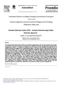
Energy consumption time series are recorded by smart meters at the regular interval of an hour or fewer [21, 24]. Smart meters read the detailed energy consumption in a real-time or near real-time fashion, which provides the opportunity to monitor timely unusual events or consumption behaviors [22, 23, 25]. However, the enabling detection technologies combining smart meters typically using data mining technologies, which require large amounts of training data sets, and significantly complex systems. In a typical application of data mining to anomaly detection, the detection models are produced off-line because the learning algorithms have to process tremendous amounts of data [17]. The produced models are naturally used by off-line anomaly detections, i.e., analyzing consumption data after being loaded into an energy management system (EMS). However, we argue that effective anomaly detection should happen real-time in order to minimize the compromises to the use of energy. The efficiency of updating the detection model and the accuracy of the detection results are the important consideration for constructing a real-time anomaly detection system. In this paper, we propose a statistical anomaly detection algorithm to detect the anomalous daily electricity consumption. The anomaly detection is based on consumption patterns, which are usually quite similar for a customer, such as in weekdays, or in weekends/holidays. We define the anomaly as the difference from the expected consumption as illustrated in Fig. 1. The proposed detection method is not limited to daily patterns, but can be easily adapted to the periodicity of the underlying data set. It is also important to note that our methods are applicable not only to electricity consumption, but other energy types of consumption, such as gas, water, and heat. This is caused by the general nature of time series data, and the generality of our detection methods presented in this paper.
Fig. 1. Daily consumption pattern and anomalies
To detect anomalies in time and obtain a better accuracy, we make use of the socalled Lambda architecture [29], that can detect anomalies near real-time, and can efficiently update detection models regularly according to a user-specified time interval. A lambda architecture enables real-time updates through a three-layer structure, including speed layer (or real-time layer), batch layer and serving layer. It is a generic system architecture for obtaining near real-time capability, and its three layers use different technologies to process data. It is well-suited for constructing an anomaly detection system that requires real-time anomaly detection and efficient model refreshment (we will detail it in the next section). To support big data capability, we choose Spark Streaming as the speed layer technology for detecting anomalies on a large amount of data streams, Spark as the batch layer technology for computing anomaly detection models,
and PostgreSQL as the serving layer for saving the models and detected anomalies; and sending feedbacks to customers. The proposed system can be integrated with smart meters to detect anomalies directly. We make the following contributions in this paper: 1) we propose the statistical-based anomaly detection algorithm based on customers’ history consumption patterns; 2) we propose making use of the lambda architecture for the efficiency of the model updating and real-time anomaly detection; 3) we implement the system with a lambda architecture using hybrid technologies; 4) we evaluate our system in a cluster environment using realistic data sets, and show the efficiency and effectiveness of using the lambda architecture in a real-time anomaly detection system. The rest of this paper is organized as follows. Section 2 discusses the anomaly detection algorithm used in the paper. Section 3 describes the implementation of the lambda detection system. Section 4 evaluates the system. Section 5 surveys the related works. Section 6 concludes the paper and provides the direction for the future works.
2
Preliminaries
2.1
Anomaly Detection Model
The used anomaly detection model is a combination of a short-term energy consumption prediction algorithm, called periodic auto-regression with eXogenous variables (PARX) [3], and Gaussian statistical distribution. We now first describe the PARX algorithm, which is used to predict the daily consumption. Generally speaking, residential electricity consumption is highly correlated to temperature. For example, in winter, electricity consumption increases since the temperature decreases because of the heating needs. In summer, electricity consumption increases when the temperature is higher because of cooling loads. The daily consumption pattern of a customer typically demonstrates the periodic characteristics, due to the living habit of the customer, e.g., the morning peak appears between 7 and 8 o’clock if a customer usually gets up at 7 o’clock; and evening peak appears between 17 and 20 o’clock (due to cooking and washing) if the customer gets home at 5 o’clock after work. The PARX model, thus, uses a daily period, taking 24 hours of the day as the seasons, i.e., t = 0...23, and uses the previous p days’ consumptions at the hour at t for auto-regression. The PARX model at the s-th season and at the n-th period is formulated as p
Ys,n = ∑ αs,iYs,n−i + βs,1 XT 1 + βs,2 XT 2 + βs,3 XT 3 + εs , s ∈ t
(1)
i=1
where Y is the data point in the consumption time-series; p is the number of order in the auto-regression; XT 1, XT 2 and XT 3 are the exogenous variables accounting for the weather temperature, defined in the equations of (2); α and β are the coefficients; and ε is the value of the white noise. ( T − 20 XT 1 = 0
if T > 20 XT 2 = otherwise
( 16 − T 0
if T < 16 XT 3 = otherwise
( 5−T 0
if T < 5 (2) otherwise
The variables represent the cooling (temperature above 20 degrees), heating (temperature below 16 degrees), and overheating (temperature below 5 degrees), respectively. The anomaly detection algorithm is of using unique variate Gaussian distribution, described in the following. Given the training data set, X = {x1 , x2 , ..., xn } whose data points obey the normal distribution with the mean µ and the variance δ2 , the detection function is defined as (x−µ)2 1 − (3) p(x; µ, δ) = √ e 2δ2 δ 2π where µ = 1n ∑ni=1 xi and δ2 = 1n ∑ni=1 (xi − µ)2 . For a new data point, x, this function computes its probability density. If the probability is less than a user-defined threshold, i.e., p(x) < ε, it is classified as an anomaly, otherwise, it is a normal data point. In our model training process, we compute the L1 distance between the actual and predict consumptions, i.e., ||Yt − Yˆt ||, where Yt is the actual hourly consumption at the time t, and Yˆt is the predict hourly consumption at the time t. The predict hourly consumption, Yˆt , is computed using the PARX model in Equation 1. We find that the L1 distances observe to a log-normal distribution (see Section 4.2). Therefore, the x in the normal distribution will be the log value of the distance, i.e., ln||Yt − Yˆt ||. 2.2
Lambda Architecture
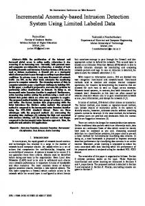
We now introduce the lambda architecture used in our anomaly detection system. As mentioned in Section 1, the lambda architecture consists of three layers, including speed layer, batch layer and serving layer, illustrated in Fig. 2. The speed layer directly ingests data streams from data sources, processes them, and continuously updates the results into the real-time views in the database in the serving layer. The speed layer does not keep any history records, and typically uses main memory based technologies to analyze the incoming data. In contrast, the batch layer runs iteratively and starts from the beginning of the data set once a batch job has finished. When a batch job starts, all the available data in the batch layer storage will be reprocessed. Therefore, the data arriving after the job starts will be processed by the next job. Since all the data are analyzed in each iteration, each of the new result views will replace its predecessor. As the batch layer does not rely on incremental processing, it is robust to any system failures, which the batch job simply processes all the available data sets in each iteration. The speed and batch usually use different technologies because of their distinct requirements regarding read and write operations. Any query against the data is answered through the serving layer, i.e., the query processor queries both the views from the speed and the batch layers, and merges them. The lambda architecture itself is only a paradigm. The technologies with which the different layers are implemented are independent of the general idea. The speed layer only deals with new data and compensates for the high latency updates of the batch layer. It can typically leverage stream processing systems, such as Storm, S4, and Spark Streaming, etc. The batch layer needs to be horizontally scalable and supports random reads, where the technologies like Hadoop with Cascading, Scalding, Pig, and Hive, are suitable. The serving layer requires a system with the ability to perform fast random reads and writes. The system can be a high-performance RDBMS (e.g., PostgreSQL),
Fig. 2. Lambda architecture
an in-memory data store (e.g., Redis, or Memcache), or a high scalable NoSQL system (e.g., HBase, Cassandra, ElephantDB, MongoDB, or DynamoDB).
3 3.1
IMPLEMENTATION System Overview
We now describe the implementation of the anomaly detection system. We choose Spark Streaming, Spark, and PostgreSQL as the speed layer, batch layer and serving layer technology, respectively (see Fig. 3). The system employs Spark to compute the models for anomaly detection, which reads the data from the Hadoop distributed file system (HDFS) in the batch layer. The batch job runs at a regular time interval, computes, and updates the detection models to the table in PostgreSQL database. Spark Streaming is used to process real-time data streams, e.g., directly reads the readings from smart meters, and detects abnormal consumption with the detection algorithm. The detection algorithm always uses the latest models getting from the PostgreSQL database. Spark Stream writes the detected anomalies back to the PostgreSQL database, which will be used for the notification of customers.
Fig. 3. The anomaly detection system
3.2
Training Anomaly Detection Models
We employ Spark to train the detection models by running regular batch jobs. All the consumption data from smart meters are written to the append-only HDFS. In each iteration of the batch jobs, Spark uses all the available data in HDFS to compute the detection models. The use of Spark and HDFS supports the computation of the models based on scalable data sets. Since they both are the distributed computing technology,
the computation can be finished within a certain time limit, meaning that the detection algorithm can always use the latest models. Fig. 4 illustrates the training process of generating PARX and Gaussian models using energy consumption and weather temperature time series at the season from 0 to 23. That is, for each season we create a new time series, e.g., for s = 0, the time series is created using the readings at 0 o’clock of all days. Then the Equation 1 is used to compute the PARX model (or parameters), and to compute the Gaussian model, i.e., N(µ, δ2 ). Therefore, there are 24 PARX and 24 Gaussian models in total.
Fig. 4. Process of training detection models
Algorithm 1 gives more details about the implementation. This algorithm computes the anomaly detection models with the given training time series collection T S , weather temperature time series ts0 , and auto-regression order p. Each time series in T S represents the hourly energy consumption of a customer. To compute the detection models for each season s, we first need to create a new consumption time series and a new temperature time series (see line 7), then use the two new time series to compute the PARX model (see line 8). According to our analysis in Section 4.2, the L1 distances between predict consumption and actual consumption at season s for all days observes to a log-normal distribution. Therefore, we compute Gaussian statistical model based on the L1 distance log values (see line 12-18). The total number of PARX models for all the time series is ||T S || × 24, which is same as the number of the Gaussian models. In the end, all the models are updated to the PostgreSQL database that will be used for the online anomaly detection in the speed layer. The implementation is a Spark program. The consumption time series, as well as temperature time series, are read into the distributed memory as resilient distributed datasets (RDDs), which are fault-tolerant, immutable and partitioned parallel data structures that can be operated in parallel, e.g., by using the operators, including map, reduce, groupByKey, filter, collect, etc [35]. To generate the new time series, we use the groupByKey operator to aggregate the consumption series by the composite key of meter ID and season (or hours); while use only the season as the key to the temperature time series. Then, we merge the generated time series by the join operator on the key of the season. The PARX, in fact, can be regarded as a multi-linear regression model, which simply takes the auto-regressors and the exogenous variables as the independent variables. We, then, apply the multiple linear regression function from the Spark machine learning library, MLib [30], to compute the coefficients. For all of these operations, the transformation functions are directly applied on RDDs for data processing.
Algorithm 1 Training of the anomaly detection models function T RAIN(TimeSeriesCollection T S , TemperatureTimeSeries ts0 Order p) M ← {} . Initialize the collection of PARX parameters N ← {} . Initialize the collection of the statical model parameters for all ts ∈ T S do id ← Get the unique identity of ts for all s ∈ 0...23 do tsc ,tst ← Construct a new consumption time series using ts, and a new temperature time series tst using ts0 at the season of s 8: α1 , ..., α p , β1 , β2 , β3 ← Compute PARX model using tsc and tst 9: Insert (id, s, α1 , ..., α p , β1 , β2 , β3 ) into M 10: L ← {} 11: D ← Get the days of ts 12: for all d ∈ D do 13: vˆ ← Compute the predict reading of the season s using PARX 14: v ← Get the actual hourly reading from ts of the day d 15: l ← Compute the ln value of L1 distance of the day d, ln(||vˆ − v||) 16: Add l into L 17: µ, β ← Compute the mean and standard deviation using the normal distribution statistical model on L 18: Insert (id, s, µ, δ) into N return M , N
1: 2: 3: 4: 5: 6: 7:
3.3
Real-time Anomaly Detection
The real-time anomaly detection is carried out in the speed layer. Algorithm 2 describes the anomaly detection process, which is self-explanatory. First, the detection algorithm reads meter readings from all the incoming data streams, and reads the weather temperature and detection models from the PostgreSQL database each hour. For each data stream, the algorithm predicts the reading using the PARX algorithm, with the precomputed parameters, the previous p day’s readings at the current hour, i.e., the season s, and weather temperature (see line 4–7). Then, the algorithm calculates the log value of the L1 distance between the predict and the actual readings, then uses it compute the probability using the Gaussian model (see line 8-10). In the end, the algorithm decides whether the current reading is an anomaly or not based on the computed probability value, i.e., if its value is below the user-defined threshold, ε. If the current reading is classified as an anomaly, it will be written into the database for the customer notification (see line 11–12). Algorithm 2 Real-time anomaly detection 1: 2: 3: 4: 5: 6: 7: 8: 9: 10: 11: 12:
function D ETECT(CurrentReadingCollection V , Temperature t, PredictModel M , StaticalModel N , Threshold ε ) R ← {} . Initialize the detection results for all v ∈ V do id ← Get the unique identity of v s ← Get the season of v α1 , ..., α p , β1 , β2 , β3 ← Get the parameters from M by id vˆ ← Compute the predict reading at s using PARX with the parameters, the p days’ readings at s, and temperature t x ← ln||vˆ − v|| . Compute the ln value of L1 distance at the season s µ, δ ← Get the statical model parameters from N by id and s p ← Compute the probability using the normal distribution function, if p < ε then Add (id, s, p, v, v) ˆ into R return R
(x−µ)2 − √1 e 2δ2 δ 2π
We implement the algorithm to process the real-time data on Spark Streaming. Spark Streaming allows for continuous processing via short interval batches, and its basic data abstraction is called discretized streams (D-Streams), a continuous stream of data [36]. The data are received in each interval batch, hourly in our case, and operations will run upon the data for doing transformations, such as filter unnecessary attribute values, extracting the hour from the timestamp, etc. (see Fig. 5). When using the PARX for prediction, we fetch the previous p days’ readings of the current hour for auto-regression. For example, in Fig. 5 we set the order, p = 3, therefore, the window size is set to 72 hours (i.e., 3 days) to keep the past three days’ readings at the particular hour within the same window (e.g., the RDDs colored by green). This is done by using the window function, reduceByKeyAndWindow(func, windowLength, slideInterval), to aggregate the data with specified key, window length and slide interval (e.g., meter ID and season as the composite key in this case, windowLength = 72 hours and slideInterval = 1 hour). In the underlying, Spark uses the data checkpointing mechanism to keep the past RDDs in HDFS. At the beginning of each interval batch, the data models are read from the PostgreSQL database in the serving layer, and broadcast to all DStreams. Therefore, the detection program always uses the latest models to detect anomalies.
Fig. 5. Slide windows in the real-time anomaly detection
4 4.1
EVALUATION Experimental settings
In this section, we will evaluate the effectiveness and the scalability of our anomaly detection system. We conduct the experiments in a cluster with 17 servers. Five servers are used for running the speed layer, while twelve servers are used for the batch layer. We also exploit one of the servers in the speed layer as the serving layer for managing the detection models and sending anomaly detection messages. All the servers have the identical settings, configured with an Intel(R) Core(TM) i7-4770 processor (3.40GHz, 4 Cores, hyper-threading is enabled, two hyper-threads per core), 16GB RAM, and a Seagate Hard driver (1TB, 6 GB/s, 32 MB Cache and 7200 RPM), running Ubuntu 12.04 LTS with 64bit Linux 3.11.0 kernel. The serving layer uses PostgreSQL 9.4 database with the settings “shared buffers=4096MB, temp buffers=512MB, work mem=1024MB, checkpoint segments=64” and default values for the other configuration parameters.
We have a real-world residential electricity consumption data set (27,300 time series), which will be used to evaluate anomaly detection accuracy. The time-series has a two-year length and hourly resolution. To evaluate the scalability, we use the synthetic data set generated by our data generator seeded by the real-world data. The size of data tested in the cluster environment is scaled up to one terabyte, corresponding to over twenty million time series. 4.2
Anomaly Detection Accuracy
We start by evaluating the accuracy of our anomaly detection system using a randomlyselected time series from the real-world data set. To provide a basis for comparison, we perform the anomaly detection using a standard boxplot analysis as well. Boxplot is a quick graphic approach for examining data sets, and has been used for decades. A boxplot uses five parameters to describe a numeric data set, including lower fence, lower quartile, media, upper quartile and upper fence (see Fig. 6). According to Fig. 6, a boxplot is constructed by drawing a rectangle between the upper and lower quartiles with a solid line indicating the median. The length of the box is called interquartile range, IQR. The sample data points lying outside the fences, 1.5 ∗ IQR, are classified as the outliers, which has been indicated to be acceptable for most situations [10]. To align boxplot with our detection method, we test the anomalies based on the 24 seasons. There are 17,520 data points in total in the selected time series. Fig. 7 shows the boxplot result where the blue points located on the top of the upper fence represent the anomalies, a total of 1,260 data points. Since the boxplot approach is merely able to detect energy consumption lying unusually far from the main body of the data, it is difficult to determine which ones are the true anomalies, and to identify the potential reasons for these anomalies because there are too many false positives.
Fig. 6. Box plot
Fig. 7. Anomaly detection using box plot
We now use the proposed detection algorithm to analyze the same time series. Fig. 8 depicts the distribution of the L1 distances of a season by the histogram. As shown, the distribution has the shape of a log-normal distribution. We have checked the L1 distance distributions for all the 24 seasons, and found that they all share a similar shape. This is the reason that we choose log-normal distribution in our statistical-based anomaly detection. Besides, we test the anomalies by treating all the days the same, and differently, i.e., discriminating the days into workdays, weekend & holidays. Moreover, we increase the threshold value, ε, from 0.05 to 0.15, and do the evaluation. The results in Fig. 9 demonstrate that the detection identifies more anomalies for treating all the
Fig. 8. Log-normal distributions Fig. 9. Anomaly detection using Fig. 10. Impact of detection across the L1 distances PARX and statistical method model update frequency
days the same than differently. The reason is that during weekends and holidays, people tend to stay at home more time, thus use more energy. The consumptions are more likely higher than the weekdays. For the threshold parameter, its value is for classifying a usual or unusual reading. According to the results, if the value increases, the number of detected anomalies changes significantly. For the real-world deployment of this system, the threshold value can be set by the residents to decide when to receive anomaly alerting messages. We now evaluate the impact of the model update frequency on the detection accuracy. We use half-year’s time series as the initial data set to train the detection models. We design the following three scenarios for the model update: 1) update per day; 2) update per 10 days behind the detection; and 3) without update. We measure the detected anomalies of the three scenarios by treating all days the same. According to the results in Fig. 10, the frequent updates of the models help to decrease the detected anomalies. It is due to the improvement of the prediction accuracy of the PARX model. Thus, less large L1 distances are identified as the anomalies. However, although the update frequency does help to determine the real anomalies, the results do not show a big difference if the models are updated within a certain short-time interval, e.g., the results of the scenario 1) and 2). In the end, we compare our approach with the boxplot, and the result shows that the number of the anomalies reported by the PARX prediction and statistical method can be decreased notably. This increases the chance to determine accurately real anomalies for an energy consumption time series. 4.3
System Scalability
We now evaluate the scalability of our anomaly detection system. As our system can scale-out and to efficiently cope with large amounts of data, we vary both the number of executors and the volume of the input data in the following experiments. Scale-out experiment. Parallel processing is a key feature of the proposed system. To evaluate the scalability of our implementation, we conduct the experiment by varying the number of executors in Spark. In this experiment, we use a fix-sized synthetic data set with eight million time series of a one-year length (275GB), which were generated by our data generator seeded the real-world data. Since we are interested in the real-time and batch capability of our system, we test the real-time anomaly detection
Fig. 11. Batch model training
Fig. 12. Real-time detection
Fig. 13. Size-up experiment
and batch model training separately. We first test the batch capability by running the training program with the number of executors increased from 8 to 256. We run each test repeatedly for ten times, and record its execution times. The results are depicted by the boxplot shown in Fig. 11. According to the results, the execution time and the time variance decrease when more executors are added. But, when the number reaches 64, the increasing parallelism does not speed up the batch processing further, which is due to the overhead of the Spark master when managing a large number of executors. We conduct the real-time anomaly detection on Spark Streaming, and likewise, we scale the number of executors from 8 to 256. Fig. 12 shows the results, which indicate that the variance of execution time is larger than the batch model training. It might be due to the variability of real-time batch executions on Spark Streaming when doing the anomaly detection for each hour. Increased data load experiment. To evaluate the scalability of the algorithms over large volumes of data, we compare different workloads. According to the above experiments, the optimal number of parallel executors for model training and anomaly detection are 64 and 128, respectively. We use the optimal executor number (the memory of executor is configured to 4GB) in our experiments, but vary the number of time series from 8 to 24 million (corresponding to the size from 275GB to 825GB). The processing times of varying data workloads are displayed in Fig. 13. We observe that both of the training and detection processes can scale near linearly with the quantity of the time series. The time of detection, in this case, is the total execution time of handling all the time series of a one-year length, e.g., it takes less than two minutes to finish eight million time series with the optimized settings. The average time of each realtime batch only takes a few seconds (recall that a batch in Spark Streaming processes the data of each hour). In the real-world deployment, the detection program can be set to run every hour to inspect hourly smart meter readings. According to the results, the anomaly detection system has a very good scalability which can meet the fast-growth of smart meter data. Unlike the anomaly detection, the training process uses the full set of the data to generate new models each time. Anomaly detection, instead, is performed for each hour where Spark Streaming runs periodical batch (or impulse) to process the data, which needs more time in overall. The training and detection programs can be deployed either in different clusters or the same cluster. If deployed in the same cluster, it is necessary to allocate computing resources in a reasonable way. For example, since the batch job
takes a much longer time, it can be scheduled to run immediately after the anomaly detection job. A scheduling system is, thus, necessary, and this will leave to our future work.
5
RELATED WORKS
Anomaly energy consumption detection. Anomaly detection is an important aspect in energy consumption time series management. Chandola et al. present a survey of different anomaly detection techniques in various application domains including energy [6]. Statistical and data mining are the commonly used techniques for discovering abnormal consumption behaviors [14]. Statistical methods are based on modeling data using distributions, and see if the data under test observes to the distributions. Accordingly, the approaches presented in this paper combine PARX and log-normal distribution function to detect anomalies in energy consumption time series. Jakkula and Cook use statistics and clustering to identify outliers in power datasets collected from smart environments [13], but they have not considered the impact of the exogenous variables, e.g., weather temperature, on the electricity consumption. Linear regression can extract time series features when the dependent variables are well-defined [27]. The early experience of identifying outliers in linear regression is through setting a threshold limit, but this yields many false positives for large data sets [16]. Adnan et al. combine linear regression with clustering techniques for getting better results [1]. Zhang et al. [37] further use piecewise linear regression to fit the relation between energy consumption and weather temperature. The results obtained are more favorable than entropy and clustering methods. But, their approach does not take the changes of consumption pattern into account. Brown et al. use K-nearest neighborhood (KNN) in fast kernel regression to predict electricity consumption [4], which requires large datasets. The resulting models are static, thus it is not preferable for online anomaly detection and the situation when consumption pattern is changed. Nadai et al. combine ARIMA and adaptive artificial neural network (ANN) to detect anomaly consumption [9] using a relatively small data set that is from a few buildings. In comparison, we propose the prediction and statistical anomaly models and combine with the lambda architecture for supporting regular model refreshment, and real-time anomaly detections. Besides, the proposed approach can handle scalable data sets, and consumption pattern changing owing to its use of the PARX model. Batch and stream processing on big data. Batch and realtime/stream processings have attracted much research effort in recent year, with the popularity of Internet of Things (IoT). Liu et al. make a survey of the existing stream processing systems, and discuss the potential technologies used for lambda architecture [20]. Cheng et al. propose a smart city data platform that supports both batch and real-time data processings [7], and they suggest that anomaly detection should be implemented as the chief component of any platform for processing sensor data. Different to proposing the generic lambda architecture [29], Preuveneers et al. [31] and Gao [11] present the big data architectures for processing domain-specific big data, including health care, context-aware user authentication and social media. Schneider et al. study batch data and streaming data anomaly detection, respectively [32]. The used detection model, however, is static,
and the use case is different to ours which employs the batch job to update the models only while use the real-time job to detect the anomalies online in data streams. The use of lambda architecture. Lambda architecture has attracted a growing interest due to its mix capabilities to process both real-time and batch data. Sequeira et al. use lambda architecture in an industrial EMS solution with cloud computing capabilities [33]. Kroßet al. develop on-demand stream processing within the lambda architecture to optimize computing resource usage in a cluster [15]. Martnez-Prieto et al. adapts the lambda architecture in semantic data processing [28]; Liu et al. applies it to smart grid complex event processing (CEP) [19]; Villari et al. proposes AllJoyn Lambda, the platform for managing embedded devices of smart homes [34]; and Hasani et al. use it for real-time big data analytics [12]. Besides, the works [5, 20] both give an extensive review of the technologies of the lambda architecture. Although there are various use cases of the lambda architecture, we focus on its use in the particular use case, anomalous energy consumption detection. More specifically, we use it in the model update and the real-time anomaly detection, which is significant to the large deployment of smart meters and sensors of IoT today.
6
CONCLUSIONS AND FUTURE WORK
Analyzing and detecting anomalies is an important task for live energy consumption data while the improvement of detection accuracy and scalability is challenging. In this paper, we applied the novel lambda architecture technique to an anomaly detection system in order to support batch updates of the detection models, and real-time detection. We have proposed the detection algorithm for finding the anomalies based on one’s history consumption pattern via the supervised learning and statistical algorithms. Furthermore, the system supports personalized alerting service by setting a threshold value for suspicious energy consumption. We have evaluated the accuracy of the anomaly detection algorithm on a real-world data set, and the scalability of the system on a large synthetic data set. The results have validated the effectiveness and the efficiency of the proposed system with a lambda architecture. For the future work, we will implement a scheduling system that can coordinate the running of the batch and real-time jobs within the same cluster. We intend to explore the ways to detect a greater range of anomalies, such as missing values, negative energy consumption and device errors. Besides, we plan to support additional types of data, such as gas, heating and water data, and to implement the corresponding detection algorithm. Acknowledgements. This research was supported by the CITIES project (NO. 103500027B) funded by Innovation Fund Denmark.
References 1. Adnan, R., Setan, H., Mohamad, M. N.: Multiple Outliers Detection Procedures in Linear Regression. Matematika. 19, 29–45 (2003) 2. Akyildiz, I. F., Su, W., Sankarasubramaniam, Y., Cayirci, E.: Wireless Sensor Networks: A Survey. J. Computer Networks. 38(4), 393–422 (2002) 3. Ardakanian, O., Koochakzadeh, N., Singh, R.P., Golab, L., Keshav, S.: Computing Electricity Consumption Profiles from Household Smart Meter Data. In: EDBT/ICDT Workshops, vol. 14, pp.140–147 (2014)
4. Brown, M., Barrington-Leigh, C., Brown, Z.: Kernel Regression for Real-Time Building Energy Analysis. J. Building Performance Simulation. 5(4), 263–276 (2011) 5. Casado, R., Younas, M.: Emerging trends and technologies in big data processing. Concurrency and Computation: Practice and Experience 27(8), 2078–2091 (2015) 6. Chandola, V., Banerjee, A., Kumar, V.: Anomaly Detection: A Survey. ACM Computing Surveys, 41(3), 15 (2009) 7. Cheng, B., Longo, S., Cirillo, F., Bauer, M., Kovacs, E.: Building a Big Data Platform for Smart Cities: Experience and Lessons from Santander. In: IEEE International Congress on Big Data, pp. 592–599. IEEE Press, New York (2015) 8. Chou, J. S., Telaga, A. S.: Real-Time Detection of Anomalous Power Consumption. Renewable and Sustainable Energy Reviews, 33, 400–411 (2014) 9. De Nadai, M., van Someren, M.: Short-Term Anomaly Detection in Gas Consumption through ARIMA and Artificial Neural Network forecast. In: IEEE Workshop on Environmental, Energy and Structural Monitoring Systems, pp. 250– 255. IEEE Press, New York (2015) 10. Frigge, M., Hoaglin, D. C., Iglewicz, B.: Some implementations of the boxplot. The American Statistician, 43(1):50–54 (1989) 11. Gao, X.: Scalable Architecture for Integrated Batch and Streaming Analysis of Big Data. Doctoral dissertation, Indiana University (2015) 12. Hasani, Z., Kon-Popovska, M., Velinov, G.: Lambda Architecture for Real Time Big Data Analytic. ICT Innovations (2014) 13. Jakkula, V., Cook, D.: Outlier Detection in Smart Environment Structured Power Datasets. In: 6th International Conference on Intelligent Environments, pp. 29–33. 2010. IEEE Press, New York (2010) 14. Janetzko, H., Stoffel, F., Mittelstdt, S., Keim, D.A.: Anomaly Detection for Visual Analytics of Power Consumption Data. Computers & Graphics. 38, 27–37 (2014) 15. Kroß, J., Brunnert, A., Prehofer, C., Runkler, T. A., Krcmar, H.: Stream Processing on Demand for Lambda Architectures. In: M. Beltrain et al. (Eds.) EPEW 2015. LNCS, vol. 9272, pp. 243–257. Springer Heidelberg (2015) 16. Lee, A. H., Fung, W. K.: Confirmation of Multiple Outliers in Generalized Linear and Nonlinear Regressions. Journal of Computational Statistics and Data Analysis. 25 (1), 55–65 (1997) 17. Lee, W., Stolfo, S. J., Chan, P. K., Eskin, E., Fan, W., Miller, M., Zhang, J.: Real Time Data Mining-Based Intrusion Detection. In: DARPA Information Survivability Conference &; Exposition II, 2001. DISCEX’01. vol. 1, pp. 89–100. IEEE Press, New York (2001) 18. Liu, F., Jiang, H., Lee, Y. M., Snowdon, J., Bobker, M.: Statistical Modeling for Anomaly Detection, Forecasting and Root Cause Analysis of Energy Consumption for a Portfolio of Buildings. In: 12th International Conference of the International Building Performance Simulation Association (2011) 19. Liu, G., Zhu, W., Saunders, C., Gao, F., Yu, Y.: Real-Time Complex Event Processing and Analytics for Smart Grid. Procedia Computer Science, 61, 113–119 (2015) 20. Liu, X., Iftikhar, N., Xie, X.: Survey of Real-Time Processing Systems for Big Data. In: 18th International Database Engineering & Applications Symposium, pp. 356–361. ACM, New York (2014) 21. Liu X, Nielsen P. S.: Streamlining smart meter data analytics. In Proc. of the 10th Conference on Sustainable Development of Energy, Water and Environment Systems, SDEWES2015.0558, 1-14, 2015. 22. Liu X, Nielsen P. S.: A Hybrid ICT-solution for Smart Meter Data Analytics. Journal of Energy, 115(3):1710–1722, 2016. 23. Liu X, Golab L, Ilyas IF.: SMAS: A Smart Meter Data Analytics System. In Proc. of ICDE, pp. 1476–1479, 2015. 24. Liu X, Golab L, Golab W, Ilyas IF: Benchmarking Smart Meter Data Analytics. In Proc. of EDBT, pp. 385–396, 2015. 25. Liu X, Golab L, Golab W, Ilyas IF, and Jin S: Smart Meter Data Analytics: Systems, Algorithms and Benchmarking. ACM Transaction of Database System (TODS), 42(1), 2016. 26. Liu X and Luo X: A Data Warehouse Solution for E-Government. International Journal of Research and Reviews in Applied Sciences, 4(1):120-128, 2010. 27. Magld, K. W.: Features Extraction Based on Linear Regression Technique. Journal of Computer Science, 8(5), 701–704 (2012) 28. Martnez-Prieto, M.A., Cuesta, C.E., Arias, M., Fernnde, J.D.: The Solid Architecture for Real-Time Management of Big Semantic Data. Future Generation Computer Systems 47, 62–79 (2015) 29. Marz, N., Warren J.: Big Data: Principles and Best Practices of Scalable Realtime Data Systems. Manning Publications Co., 1st Ed. (2013) 30. Meng, X., Bradley, J., Yavuz, B., Sparks, E., Venkataraman, S., Liu, D., Xin, D.: MLlib: Machine Learning in Apache Spark. arXiv preprint arXiv:1505.06807 (2015) 31. Preuveneers, D., Berbers, Y., Joosen, W.: SAMURAI: A Batch and Streaming Context Architecture for Large-Scale Intelligent Applications and Environments. J. of Ambient Intelligence and Smart Environments, 8(1), 63–78 (2016) 32. Schneider, M., Ertel, W., Ramos, F.: Expected Similarity Estimation for Large-Scale Batch and Streaming Anomaly Detection. arXiv preprint arXiv:1601.06602 (2016) 33. Sequeira, H., Carreira, P., Goldschmidt, T., Vorst, P.: Energy Cloud: Real-Time Cloud-Native Energy Management System to Monitor and Analyze Energy Consumption in Multiple Industrial Sites. In: 7th IEEE/ACM International Conference on Utility and Cloud Computing, pp. 529–534. IEEE Press, New York (2014) 34. Villari, M., Celesti, A., Fazio, M., Puliafito, A.: Alljoyn Lambda: An Architecture for the Management of Smart Environments in IOT. In: IEEE International Conference on Smart Computing Workshops, pp. 9–14. IEEE Press, New York (2014) 35. Zaharia, M., Chowdhury, M., Das, T., Dave, A., Ma, J., McCauley, M., Stoica, I.: Resilient Distributed Datasets: A Fault-Tolerant Abstraction for In-Memory Dluster Computing. In: 9th USENIX conference on Networked Systems Design and Implementation, pp.2–2. USENIX Association (2012)
36. Zaharia, M., Das, T., Li, H., Shenker, S., Stoica, I.: Discretized Streams: An Efficient and Fault-Tolerant Model for Stream Processing on Large Clusters. In: 4th USENIX conference on Hot Topics in Cloud Computing, pp. 10–10. USENIX Association (2012) 37. Zhang, Y., Chen, W., Black, J.: Anomaly Detection in Premise Energy Consumption Data. In: Power and Energy Society General Meeting, pp. 1–8. IEEE Press, New York (2011) 38. Zhao, H. X., Magouls, F.: A Review on the Prediction of Building Energy Consumption. Renew Sustain Energy Reviews, 16(6):3586–3592 (2012)