Optical atomic clocks - APS Link Manager - American Physical Society

REVIEWS OF MODERN PHYSICS, VOLUME 87, APRIL–JUNE 2015

Optical atomic clocks Andrew D. Ludlow,1,2 Martin M. Boyd,1,3 and Jun Ye1 1

JILA, National Institute of Standards and Technology and University of Colorado, Boulder, Colorado 80309, USA 2 National Institute of Standards and Technology (NIST), 325 Broadway, Boulder, Colorado 80305, USA 3 AOSense, 929 E. Arques Avenue, Sunnyvale, California 94085, USA

E. Peik4 and P. O. Schmidt4,5 4

Physikalisch-Technische Bundesanstalt, Bundesallee 100, 38116 Braunschweig, Germany Institut für Quantenoptik, Leibniz Universität Hannover, Welfengarten 1, 30167 Hannover, Germany

5

(published 26 June 2015) Optical atomic clocks represent the state of the art in the frontier of modern measurement science. In this article a detailed review on the development of optical atomic clocks that are based on trapped single ions and many neutral atoms is provided. Important technical ingredients for optical clocks are discussed and measurement precision and systematic uncertainty associated with some of the best clocks to date are presented. An outlook on the exciting prospect for clock applications is given in conclusion. DOI: 10.1103/RevModPhys.87.637

PACS numbers: 32.30.−r, 06.30.Ft, 37.10.Jk, 37.10.Ty

4. Stark shift 5. Blackbody radiation shift D. Ionic candidates and their electronic structure E. Quantum logic spectroscopy of Alþ 1. Quantum logic spectroscopy 2. Clock operation 3. Experimental achievements of the Alþ clocks 4. Systematic shifts of the Alþ clocks F. Other optical ion frequency standards 1. Calcium 2. Strontium 3. Ytterbium 4. Mercury 5. Barium 6. Indium VI. Neutral Atom Ensemble Optical Frequency Standards A. Atomic candidates: Alkaline earth(-like) elements B. Laser cooling and trapping of alkaline earth(-like) atoms C. Free-space standards D. Strong atomic confinement in an optical lattice 1. Spectroscopy in the well-resolved-sideband and Lamb-Dicke regimes 2. The magic wavelength 3. Spectroscopy of lattice confined atoms 4. Ultrahigh resolution spectroscopy E. Systematic effects in lattice clocks 1. Optical lattice Stark shifts 2. Zeeman shifts 3. Stark shift from blackbody radiation 4. Cold collision shift 5. Stark shift from interrogation laser 6. Doppler effects 7. dc Stark shifts 8. Other effects

CONTENTS I. Introduction 638 A. Ingredients for an atomic frequency standard and clock 638 B. Characterization of frequency standards 639 C. Scope of paper 639 II. Desiderata for Clocks: Quantum Systems with High-frequency, Narrow-line Resonances 639 A. Stability 639 B. High-frequency clock candidates 640 C. Systematic effects 641 1. Environmental perturbations 641 a. Magnetic fields 641 b. Electric fields 641 2. Relativistic shifts 642 a. Doppler shifts 643 b. Gravitational redshift 643 III. Spectrally Pure and Stable Optical Oscillators 643 A. Laser stabilization technique 643 B. Remote distribution of stable optical sources 644 C. Spectral distribution of stable optical sources 645 IV. Measurement Techniques of an Optical Standard 646 A. Clock cycles and interrogation schemes 646 B. Atomic noise processes 647 C. Laser stabilization to the atomic resonance 648 V. Trapped-ion Optical Frequency Standards 649 A. Trapping ions 650 1. Paul traps 651 2. Linear ion traps 651 B. Cooling techniques and Lamb-Dicke regime 653 C. Systematic frequency shifts for trapped ions 653 1. Motion-induced shifts 653 2. Zeeman effect 654 3. Quadrupole shift 654

0034-6861=2015=87(2)=637(65)

637

655 655 656 657 657 659 660 661 663 663 663 663 664 664 664 664 664 665 667 667 667 669 670 671 671 672 673 674 675 676 676 677 677

© 2015 American Physical Society

638

Ludlow et al.: Optical atomic clocks

F. Optical lattice clocks based on fermions or bosons G. Lattice clock performance 1. Clock stability 2. Systematic evaluations 3. Absolute frequency measurements VII. Applications and Future Prospects A. Primary standards and worldwide coordination of atomic time B. Technological applications C. Optical clocks for geodetic applications D. Optical clocks in space E. Variation of fundamental constants F. Quantum correlations to improve clock stability G. Designer atoms H. Active optical clocks and superradiant lasers I. Many-body quantum systems J. Atomic clocks with even higher transition frequencies Acknowledgments References

677 678 678 680 681 682 683 684 684 685 686 687 689 689 690 691 692 692

might be based on an optical transition (Gill, 2011), but even now, accurate optical frequency standards are becoming de facto secondary standards (CIPM, 2013). Aside from the benefits of these practical applications, for scientists there is the additional attraction of being able to precisely control a simple quantum system so that its dynamics evolve in its most elemental form. One exciting possibility is that the evolution may not be as originally expected. For example, an area of current interest explores the idea that the relative strengths of the fundamental forces may change in time; this would indicate new physics (Bize et al., 2004; Fischer et al., 2004; Blatt et al., 2008; Rosenband et al., 2008b). Comparing clocks based on different atoms or molecules may someday make such effects observable. Another example is the application of clock precision to the study of many-body quantum systems (Martin et al., 2013; Rey et al., 2014). A. Ingredients for an atomic frequency standard and clock

I. INTRODUCTION

An 1879 text written by Thomson (Lord Kelvin) and Tait (Thomson and Tait, 1879; Kelvin and Tait, 1902; Snyder, 1973) included the following: “The recent discoveries due to the kinetic theory of gases and to spectrum analysis (especially when it is applied to the light of the heavenly bodies) indicate to us natural standard pieces of matter such as atoms of hydrogen or sodium, ready made in infinite numbers, all absolutely alike in every physical property. The time of vibration of a sodium particle corresponding to any one of its modes of vibration is known to be absolutely independent of its position in the Universe, and it will probably remain the same so long as the particle itself exists.” Although it took a while to realize, this idea attributed to Maxwell (Thomson and Tait, 1879; Kelvin and Tait, 1902) is the basic idea behind atomic frequency standards and clocks. In this review, we focus on frequency standards that are based on optical transitions, which seems to be implicit in the text above. Optical frequency references have certain advantages over their predecessors at microwave frequencies; these advantages are now starting to be realized. The need for more accurate and precise frequency standards and clocks has continued unabated for centuries. Whenever improvements are made, the performance of existing applications is enhanced, or new applications are developed. Historically, the prime application for clocks has been in navigation (Major, 2007; Grewal, Andrews, and Bartone, 2013), and today we take for granted the benefits of global navigation satellite systems (GNSS), such as the global positioning system (GPS) (Kaplan and Hegarty, 2006; Rao, 2010; Grewal, Andrews, and Bartone, 2013). With the GPS, we can easily navigate well enough to safely find our way from one location to another. We look forward to navigation systems that will be precise enough to, for example, measure small strains of the Earth’s crust for use in such applications as earthquake prediction. In addition, frequency standards provide the base unit of time, the second, which is by definition derived from the electronic ground-state hyperfine transition frequency in caesium. Eventually the definition of the second Rev. Mod. Phys., Vol. 87, No. 2, April–June 2015

All precise clocks work on the same basic principle. First we require a system that exhibits a regular periodic event; that is, its cycles occur at a constant frequency, thereby providing a stable frequency reference and a basic unit of time. Counting cycles of this frequency generator produces time intervals; if we can agree on an origin of time then the device subsequently generates a corresponding time scale. For centuries, frequency standards were based on celestial observations, for example, the Earth’s rotation rate or the duration of one orbit of the Earth about the Sun (Jespersen and Fitz-Randolph, 1999). For shorter time scales other frequency standards are desirable; classic examples include macroscopic mechanical resonators such as pendulum clocks, John Harrison’s famous spring based clocks for maritime navigation, and starting in the early 20th century quartz crystal resonators (Walls and Vig, 1995; Vig, 1999). However, each of these frequency standards had its limitations; for example, the Earth’s rotation frequency varies in time, and the frequency stability of macroscopic mechanical resonators is limited by environmental effects such as changes in temperature. As Maxwell realized, an atom can be an ideal frequency standard because, as far as we know, one atom is exactly identical to another atom of the same species. Therefore, if we build a device that registers the frequency of a natural oscillation of an atom, say the mechanical oscillations of an electron about the atom’s core, all such devices will run at exactly the same frequency (except for relativistic effects discussed later), independent of comparison. Therefore, the requirement for making an atomic frequency standard is relatively easy to state: we take a sample of atoms (or molecules) and build an apparatus that produces an oscillatory signal that is in resonance with the atoms’ natural oscillations. Then, to make a clock, we simply count cycles of the oscillatory signal. Frequency standards have been realized from masers or lasers; in the context of clocks perhaps the most important example is the atomic hydrogen maser (Goldenberg, Kleppner, and Ramsey, 1960; Kleppner, Goldenberg, and Ramsey, 1962) which is still a workhorse device in many standards laboratories. However, the more common method


for achieving synchronization, and the primary one discussed here, is based on observing the atoms’ absorption. Typically, we first prepare the atom in one of the two quantum states (j1i ¼ lower-energy state, j2i ¼ upper state) associated with one of its natural oscillations. We then use a “local oscillator” that produces radiation around this oscillation frequency and direct the radiation toward the atoms. The device will be constructed so that we can detect when the atoms change state. When these state changes occur with maximum probability, then we know that the oscillator frequency is synchronous with the atoms’ natural oscillation. The details of this process are discussed later. B. Characterization of frequency standards

The degree to which we can synchronize a local oscillator’s frequency to the atoms’ natural oscillations is always limited by noise in the measurement protocol we use to establish this synchronization. In addition, although isolated atoms are in a sense perfect, their natural frequencies can be shifted from their unperturbed values by external environmental effects, typically electric and magnetic fields. Therefore, we must find a way to calibrate and correct for these “systematic” frequency shifts. Even then, there will always be errors in this correction process that we must characterize. It is therefore convenient to divide the errors into two types: statistical errors that arise from measurement fluctuations and errors in the systematiceffect corrections that are applied to the measured frequencies. We typically characterize these errors in terms of the fractional frequency errors Δf=f0 , where f 0 is the reference transition frequency and Δf is the frequency error. For statistical errors, we first suppose we have a perfect local oscillator whose frequency fs is near f c, the frequency of the clock atoms under test (fc may be shifted from f0 due to systematic effects). We assume we can measure the fractional frequency difference y ≡ ðf c − fs Þ=f0 and average this quantity over various probe durations τ. A commonly used measure of the noise performance of clocks is the Allan variance (Allan, 1966; Riehle, 2004; Riley, 2008)

639

increase with increased τ. Of course, we do not have perfect standards to compare to, so we always observe σ y ðτÞ for comparison between two imperfect clocks. Nevertheless, if we can compare three or more clocks, it is possible to extract the noise performance of each separately (Riley, 2008). Systematic errors are more challenging to document, in part because we may not always know their origin, or even be aware of them. If the measured frequency stability does not improve or becomes worse as τ increases, this indicates some systematic effect that we are not properly controlling. Even worse is that stability may improve with τ but we have not accounted for a (constant) systematic offset. Eventually such effects will likely show up when comparing different versions of the same clock; in the meantime, we must be as careful as possible to account for systematic shifts. C. Scope of paper

In this paper we are primarily interested in the physics of optical clocks, the performance and limitations of existing devices, and prospects for improvements. The status of the field has been summarized in various reviews and conference proceedings (Madej and Bernard, 2001; Gill, 2005, 2011; Hollberg, Oates et al., 2005; Maleki, 2008; Margolis, 2009; Derevianko and Katori, 2011; Poli et al., 2013), so that we will not discuss the details of all experiments. Rather, we will focus on aspects of a few high-performance clocks to illustrate the problems and issues that must be faced, as well as prospects for further advances in the state of the art. Our review covers optical atomic clocks based on both trapped single ions and many atoms. For simplicity, we use the term “atomic” clocks but of course a molecular or even a nuclear transition might be an equally viable candidate for a frequency reference. II. DESIDERATA FOR CLOCKS: QUANTUM SYSTEMS WITH HIGH-FREQUENCY, NARROW-LINE RESONANCES A. Stability

σ 2y ðτÞ ¼

1 2ðM − 1Þ

M −1 X

½hyðτÞiiþ1 − hyðτÞii 2 ;

ð1Þ

i¼1

where hyðτÞii is the ith measurement of the average fractional frequency difference over duration τ, and where we ideally assume there is no dead time between successive measurements i and i þ 1. The quantity σ y ðτÞ is commonly called the stability (but is really proportional to the instability). More efficient use of data uses overlapping samples of shorterduration measurements resulting in the “overlapping” Allan variance. This and more sophisticated measures, which can reveal the spectrum of the noise, are discussed in Riehle (2004) and Riley (2008), but the essence of the measure is contained in Eq. (1). Many sources of noise are well behaved (stationary) in the sense that if we average the output frequency of our standard for longer times, our precision on the measured frequency also improves [σ y ðτÞ decreases]. However, other sources of noise, such as systematic shifts that drift over long durations, will cause σ y ðτÞ to level off or Rev. Mod. Phys., Vol. 87, No. 2, April–June 2015

Following the basic idea outlined previously, to stabilize the frequency of a local oscillator to an atomic transition, we need to extract a sensitive discriminator signal dS=df, where S is the signal obtained from the atoms and f is the frequency of applied radiation. This signal can then be used to feed back and stabilize the oscillator’s frequency. There will be fluctuations δS on the measured signal S so that assuming no additional noise is injected during the protocol, the corresponding fractional frequency errors of the stabilized local oscillator during one feedback cycle can be expressed as δy1 ¼

δf δS : ¼ f 0 1 f0 ðdS=dfÞ

ð2Þ

From this expression we see that we want f 0 and dS=df to be as large as possible and δS as small as possible. If we denote the frequency width of the atomic absorption feature by Δf and the signal strength on resonance as S0 , we can reexpress

640


Eq. (2) as δy1 ¼ δS=S0 QκS , where Q ≡ f 0 =Δf is the Q factor of the transition and κ S ≡ ðdS=dfÞΔf=S0 is a parameter on the order of 1 that depends on the line shape. From this expression for δy1, it appears that the key parameters are signal-to-noise ratio and Q. However, we must remember that this is for a single feedback cycle, which, for a given Q, requires a measurement duration T m proportional to 1=Δf. If δS is dominated by white frequency noise we then have for repeated measurements

δf σ y ðτÞ ¼ f0

rffiffiffiffiffiffi rffiffiffiffiffiffi rffiffiffiffiffi 1 δS Tm δS Tm ¼ ; ¼ ðdS=dfÞ τ Qκ τ M f S 0 0 S 1

ð3Þ

where τ is the total measurement duration and M ¼ τ=T m is the number of successive measurements. To stabilize the local oscillator to the atomic transition, we typically first prepare the atoms in one of the two clock states, here the lower-energy state j1i. We then excite the clock transition resonance at a frequency near that which gives the maximum value of ðdS=dfÞ=δS, which is usually near or at the half-intensity points of the absorption feature. In the absence of relaxation this leaves the atom in a superposition state αj1i þ βj2i with jαj2 ≃ 1=2 and jαj2 þ jβj2 ¼ 1. In most cases discussed in this review, the observed signal is derived by use of what Hans Dehmelt termed the “electronshelving” technique (Dehmelt, 1982). Here one of the two states of the clock transition, say the lower-energy state j1i, is excited to a third level by a strongly allowed electric dipole “cycling” transition where this third level can decay only back to j1i. (We assume j2i is not excited by the cycling transition radiation.) By collecting even a relatively small number of fluorescent photons from this cycling transition, we can discriminate which clock state the atom is projected into upon measurement: if the atom is found in the state j1i it scatters many photons; if its optically active electron is “shelved” into the upper clock state j2i, fluorescence is negligible. With this method, we can detect the projected clock state with nearly 100% efficiency. When applied to N atoms simultaneously, the atomic signal and its derivative will increase by a factor of N. Upon repeated measurements of the state αj1i þ βj2i, there will be quantum fluctuations in which state the atom is projected into for each atom. These pffiffiffiffiffiffiffiffiffiffiffiffiffiffiffiffiffiffiffiffiffiffi quantum fluctuations contribute noise δS ¼ Npð1 − pÞ ¼ pffiffiffiffi N jαβj, where p ¼ jβj2 is the transition probability (Itano et al., 1993). This “projection” noise is the standard quantum noise limit in the measurements. Added noise, for example, phase noise from the probe local oscillator, will increase σ y ðτÞ. In principle, to stabilize the oscillator to the atomic reference we would need only to probe one side of the absorption line, but in practice it is often necessary to alternately probe both sides of the line and derive an error signal based on the two different values of p. Doing so reduces the influence of technical noise to the signal. The feedback servo is arranged to drive this difference to zero, in which case the mean of the two probe frequencies is equal to the atomic resonance frequency. Equation (3) still holds, but since the absorption feature will be symmetric to a high degree, probing on both sides of the line makes the Rev. Mod. Phys., Vol. 87, No. 2, April–June 2015

stabilization insensitive to slow variations in probe intensity, resonance linewidth, and detection efficiency. A particularly simple expression for σ y ðτÞ holds if we probe the resonance using the Ramsey method of separated fields (Ramsey, 1985) with free-precession time T m ∼ 1=ð2πΔfÞ and assume (1) π=2 pulse durations are short compared to T m , (2) unity state detection efficiency, (3) relaxation rates are negligible compared to 1=T m , (4) the duration required for state preparation and measurement (dead time) is negligible compared to T m , and (5) noise is dominated by quantum projection noise. In this case (Itano et al., 1993), σ y ðτÞ ¼

1 pffiffiffiffiffiffiffiffiffiffiffiffi : 2πf0 NT m τ

ð4Þ

This expression clearly shows the desirability of highfrequency, large atom numbers, long probe times (with corresponding narrow linewidths), and of course long averaging times τ. If N, T m , and τ can somehow be preserved, we see that the improvement in σ y ðτÞ is proportional to f0 . Stated another way, if N and T m are preserved, the time it takes to reach a certain measurement precision is proportional to f−2 0 , emphasizing the importance of high-frequency transitions. B. High-frequency clock candidates

The advantage of high-frequency transitions had been appreciated for decades during which clock transitions based on microwave transitions (typically hyperfine transitions) prevailed. Given the importance of high f0 and narrow linewidths, one can ask why we do not make the jump to very high frequencies such as those observed in Mössbauer spectroscopy. For example, a Mössbauer transition in 109 Ag has f 0 ≃ 2.1 × 1019 Hz and a radiative decay time τdecay ≃ 60 s corresponding to a natural Q value ≃1.3 × 1022 (Alpatov et al., 2007; Bayukov et al., 2009). Even with practical limitations, the performance of actual Mössbauer systems is still quite impressive. For example, consider the 93 keV Mössbauer transition in 67 Zn (Potzel et al., 1992). Here Q’s of 5.8 × 1014 were observed [see Potzel et al. (1992), Fig. 5] and a statistical precision of 10−18 was obtained in 5 days. As is typical in Mössbauer spectroscopy, a convenient local oscillator is obtained by using a Mössbauer emitter of the same species whose frequency is swept via the first-order Doppler shift when this source is moved at fixed velocity relative to the absorber. However, systematic effects in Potzel et al. (1992) were at a level of around 2 × 10−17 due primarily to pressure effects in the host material and dispersive line-shape effects. More importantly in the context of clocks, there is no way to observe coherence of the local oscillator; that is, there is currently no means to count cycles of the local oscillator or compare clocks based on different transitions. Moreover, comparison of Mössbauer sources over large distances (≫1 m) is intractable due to the lack of collimation of the local oscillator radiation. On the other hand, if further development of extreme ultraviolet frequency combs (Gohle et al., 2005; Jones et al., 2005; Cingöz et al., 2012) does produce spectrally narrow radiation sources in the keV


region, it will be attractive to revisit the idea of Mössbauer spectroscopy for clock applications. In the optical region of the spectrum, suitable narrowlinewidth transitions were known to exist in many atoms; however, the missing ingredients until relatively recently were (1) the availability of lasers with sufficiently narrow spectra that could take advantage of these narrow transitions and (2) a convenient method to count cycles of the stabilized (laser) local oscillators. These requirements have now been met with improved methods to lock lasers to stable reference cavities (Young et al., 1999; Ludlow et al., 2007; Dubé et al., 2009; Millo et al., 2009; Jiang et al., 2011; Kessler et al., 2012; McFerran et al., 2012; Swallows et al., 2012; Bishof et al., 2013) and the development of optical combs that provide the counters and convenient means for optical frequency comparisons (Udem et al., 1999; Diddams et al., 2000; Stenger et al., 2002; Cundiff and Ye, 2003; Hollberg, Diddams et al., 2005; Ye and Cundiff, 2005; Hall, 2006; Hänsch, 2006; Grosche, Lipphardt, and Schnatz, 2008; Schibli et al., 2008). These advances mark the beginning of high-precision clocks based on optical transitions. C. Systematic effects

To a high degree, the systematic frequency shifts encountered in optical atomic clocks are the same as for all atomic clocks. We can divide the shifts into those caused by environmental perturbations (e.g., electric or magnetic fields) and those which we might call observational shifts. The latter include instrumental effects such as servo offsets and frequency chirping in optical switches; these are apparatus specific and best examined in each experimental realization. More fundamental and universal observational shifts are those due to relativity, which we discuss later. 1. Environmental perturbations

In simple terms, we need to examine all the forces of nature and consider how each might affect the atomic transition frequencies. As far as we know, we can rule out the effects of external strong and weak forces primarily because of their short range. Gravitational effects are important but we include them when discussing relativistic shifts. The most important effects are due to electromagnetic fields. It is useful to break these into various categories, illustrated by some simple examples. Details will follow in the discussions of the various clocks. a. Magnetic fields

~ ¼ Bnˆ B are often applied purposely Static magnetic fields B to define a quantization axis for the atoms. Here we implicitly assume the field is uniform, but inhomogeneties must be accounted for in the case of spread atomic samples. Shifts from these fields often cause the largest shifts that must be corrected for but these corrections can often be implemented with high accuracy. We write f − f 0 ¼ ΔfM ¼ CM1 B þ CM2 B2 þ CM3 B3 þ ; ð5Þ Rev. Mod. Phys., Vol. 87, No. 2, April–June 2015

641

where, for small B, the first two terms are usually sufficient. The energies of clock states will depend on the atom’s magnetic moment; for example, the electron spin Zeeman effect in the 2 S1=2 → 2 D5=2 transitions of 88 Srþ gives a relatively large CM1 coefficient on the order of μB =h ≃ 1.4 × 1010 Hz=T, where μB is the Bohr magneton and h is Planck’s constant. Nevertheless, if the quantizing magnetic field is sufficiently stable, by measuring pairs of transitions that occur symmetrically around the unshifted resonance we can compensate for this shift (Bernard, Marmet, and Madej, 1998). As another example, 1 S0 → 3 P0 transitions in 87 Sr and Alþ have a much smaller value of CM1 ∼ μN =h, where μN is the nuclear magneton, thereby reducing the shifts substantially. For atoms with nonzero nuclear and electron spin, hyperfine structure will be present and both CM1 and CM2 can be significant. In this case we can often use the traditional “clock” transitions between lower states jF; mF ¼ 0i and upper states jF0 ; mF0 ¼ 0i, where F; F0 and mF ; mF0 are the total angular momenta and the projections of the angular momenta on the (magnetic field) quantization axis. For these transitions, CM1 ¼ 0 and for B → 0, ΔfM ¼ CM2 B2 can be very small. We can usually determine B to sufficient accuracy by measuring a suitable field-dependent Zeeman transition. Departures of B from its nominal value B0 might also vary in time. If these variations are slow enough it might be feasible to intermittantly measure field sensitive transitions, or even the clock transition itself, to correct for or servo-compensate the slow variations (Rosenband et al., 2007). Some isotopes of interest do not possess m ¼ 0 Zeeman sublevels because of their half-integer total angular momentum. An example is alkali-like ions without nuclear spin, where the absence of a hyperfine structure facilitates laser cooling. In this case the linear Zeeman shift of the reference transition can be compensated by interrogating two Zeeman components that are symmetrically shifted like m → m0 and −m → −m0 and determining the average of both transition frequencies. Consequently, the number of interrogations required for a frequency determination is doubled. However, this does not compromise the stability of the standard if magnetic-field fluctuations are negligible during the time between interrogations. For the operation of a 87 Sr lattice clock, alternately interrogating opposite nuclear spin stretched states of 9=2 and taking their averages greatly suppresses the first-order Zeeman shift. The second-order Zeeman shifts can be determined by fast modulation of the bias magnetic field between high and low values. By using a clock transition to directly sample and stabilize the magnetic field, the combined magnetic-field related frequency shift can be measured below 1 × 10−18 (Bloom et al., 2014; Nicholson et al., 2015). b. Electric fields

Static electric fields at the site of the atoms can arise from potential differences in surrounding surfaces caused by, for example, differences in applied potentials on surrounding conductors, surface contact potential variations, or charge buildup on surrounding insulators. Typically, clock states have well-defined parity so that first-order perturbations vanish and

642


shifts can often be calculated with sufficient precision in second-order perturbation theory. For the case of trapped ions, the static component of the electric field and corresponding Stark shifts vanish at the equilibrium position of the ions. Since they do not move, the static field at their location must be zero. For neutral atom clocks the static electric field effects are usually small; however, at the highest levels of accuracy they must be characterized (Lodewyck et al., 2012; Bloom et al., 2014) or even stabilized (Nicholson et al., 2015). Treating the quadratic Stark shift as a small perturbation of the linear Zeeman splitting, the shift of the state jγJFmi is given by (Angel and Sandars, 1968; Itano, 2000) hΔf S ðγ; J; F; m; EÞ ¼ −½2αS ðγ; JÞ þ αT ðγ; J; FÞgðF; m; βÞ gðF; m; βÞ ¼

3m2 − FðF þ 1Þ ð3cos2 β − 1Þ; Fð2F − 1Þ

jEj2 4 ð6Þ

where β is the angle between the electric field vector and the orientation of the static magnetic field defining the quantization axis. In general, the Stark shift is composed of a scalar contribution described by polarizability αS and, for levels with J > 1=2 and F > 1=2, by a tensor part that is proportional to αT . In addition to a static electric field, ac electric fields can be present from several sources. Important shifts for both neutral atoms and ions can arise from laser beams and background blackbody radiation. For neutral atoms trapped by laser fields, the frequency and polarization of light can be chosen (Katori et al., 2003; Ye, Kimble, and Katori, 2008) so that the ac Stark shifts are the same for both clock levels to a high degree and the clock frequency is nearly unshifted (see Sec. VI.D.2). For sympathetically cooled ions as in the 27 Alþ “logic clock,” the cooling light can impinge on the clock ion(s) causing Stark shifts that must be accounted for (Rosenband et al., 2008b; Chou, Hume, Koelemeij, et al., 2010). Ambient blackbody radiation shifts can be important for both neutral atoms and ions. The uncertainty in the shift can be caused by uncertainty in the effective temperature T at the position of the atoms and by uncertainties in the atomic polarizabilities. In most cases the wavelengths of electric dipole transitions originating from one of the levels of the reference transition are significantly shorter than the peak wavelength of the blackbody radiation spectrum of 9.7 μm at room temperature. Consequently, a static approximation can be used and the shift is proportional to the differential static scalar polarizability Δαs of the two levels constituting the reference transition and to the fourth power in temperature. This follows from the integration of Planck’s radiation law, yielding the mean-squared electric field hE2 ðTÞi ¼ ð831.9 V=mÞ2 ½TðKÞ=3004 . The dependence of the shift on the specific transition wavelengths and matrix elements may be accounted for in a T 2 -dependent dynamic correction factor η (Porsev and Derevianko, 2006). With these approximations, the Stark shift due to blackbody radiation (BBR) is given by hΔfBBR ¼ −

Δαs hE2 ðTÞi ½1 þ ηðT 2 Þ. 2

Rev. Mod. Phys., Vol. 87, No. 2, April–June 2015

ð7Þ

Since blackbody shifts scale as T 4 , operation at low temperatures can be advantageous; by operating near liquid helium temperatures, the shifts are highly suppressed (Itano, 2000). Tables I and V list blackbody shifts for some atoms and ions currently considered for optical clocks. For ions confined in Paul traps, the trapping rf electric fields can produce quadratic Stark shifts. These can be significant if ambient static electric fields push the ions away from the rf electric field null point in the trap. In this case the ions experience excess “rf micromotion,” oscillatory motion at the rf trap drive frequency (Berkeland et al., 1998b). The strength of the fields can be determined by observing the strength of rf micromotion induced frequency modulation (FM) sidebands of an appropriately chosen optical transition (which need not be the clock transition). As with the case of ac magnetic fields, the danger for both neutral atoms and ions is that ac electric fields may be present at the site of the atoms that otherwise go undetected. If one or both of the clock states has a quadrupole moment, shifts can arise due to ambient electric field gradients which can be strong in ion traps. In several cases of interest, one of the clock states is an atomic D level which will have such an atomic quadrupole moment that can give rise to significant shifts. In the case of atomic ions, atomic quadrupoles can couple to gradients from the Coulomb field of simultaneously trapped ions. In strongly binding traps where the ion separations are on the order of a few μm, shifts can be as large as 1 kHz (Wineland et al., 1985). Shifts from collisions are typically dominated by electric field effects. Since a precise theoretical description of these shifts is extremely complicated, experimentalists must typically calibrate them through measurements. This can be particularly important in neutral atom clocks where multiple atoms might be held in a common location and the shift is dominated by collisions between clock atoms. In this situation scattering cross sections will strongly differ between fermionic and bosonic clock atom species. This is not an issue for ions, which are well separated in the trap. Collision shifts from hot background gas atoms in vacuum can be even more difficult to characterize. At high vacuum, collisions with background gas atoms occur infrequently and it may be possible to establish a useful upper limit on collisional frequency shifts simply from the observed collision rate. Even tighter bounds can be established by a detailed analysis of the collision process using model potentials of the involved species (Gibble, 2013). For example, the largest residual gas in the ultrahigh vacuum chamber for the Sr clock is hydrogen. An estimate of the Sr-H2 van der Waals coefficients can be estimated to provide an upper bound of the background collision shift (Bloom et al., 2014). 2. Relativistic shifts

In addition to environmental effects that perturb an atom’s internal states and clock frequency, there can be errors in our determination of the clock atoms’ frequency, even when atoms are perturbation free. The most fundamental of these effects is the relativistic shifts, due to the different frames of reference of the atoms, probing lasers, and other atomic clocks.


a. Doppler shifts

Basically, we want to relate an atom’s transition frequency in its frame of reference to the frequency of the probe laser in the “laboratory frame,” which we assume is locked to the atomic transition (Chou, Hume, Rosenband, and Wineland, 2010). The frequency f of the probe laser in the laboratory frame has a frequency f0 when observed in a moving frame v∥ ; f 0 ¼ fγ 1 − c

ð8Þ

where γ ¼ ½1 − ðv=cÞ2 −1=2 , v is the atom’s velocity relative to the laboratory frame, v∥ is the atom’s velocity along the probe laser beam direction, and c is the speed of light. The clock servo ensures that the frequency of the laser in the atom’s frame equals the proper atomic resonance frequency f0 ; that is, hf 0 i ¼ f0 , where the angle brackets denote the appropriate average over the laser probe duration. If we assume that f is constant over this duration, then hfi ¼ f, and we have δf f − f0 1 −1 ¼ ¼ f0 f0 hγð1 − v∥ =cÞi

ð9Þ

f − f 0 hv∥ i hv2 i hv∥ i2 − 2 þ 2 þ Oðv=cÞ3 : ¼ c f0 c 2c

ð10Þ

or

The first term in Eq. (10), the first-order Doppler shift, can easily be the largest for clocks based on single photon transitions. Historically, the relatively large size of the firstorder Doppler shift was one of the motivations for probing confined atoms as opposed to atoms in an atomic beam. Early work on the hydrogen maser (Goldenberg, Kleppner, and Ramsey, 1960) and high resolution hyperfine spectra of trapped 3 Heþ ions (Fortson, Major, and Dehmelt, 1966) showed the advantages of confinement. Trapping for long durations would seem to guarantee hv∥ i ¼ 0. However, the distance between the mean position of the atoms and the location of the probe laser may be slowly drifting due to, for example, thermal expansion, or any change in the optical path, such as that due to a change in the index of refraction in a transmitting fiber. For example, to reach δf=f 0 < 10−17 , we must ensure hv∥ i < 3 nm=s. More generally, any effect that leads to a phase change of laser beam field experienced by the atoms can be included in this category. Fortunately, many of these effects can be compensated with Doppler cancellation schemes discussed in more detail in Sec. III.B. However, even with these measures, we must be cautious. For example, during the laser probe and feedback cycle, there might be periods where the atom’s position is correlated with the laser probe period and first-order Doppler shifts might occur. To detect and compensate for this possibility, one can probe in multiple directions (Rosenband et al., 2008b). The next two terms in Eq. (10), the so-called second-order Doppler shifts, are a form of time dilation. Although they are fairly small for room-temperature atoms, they may be difficult to characterize since the trapped atoms’ velocity distribution may not be simple. Of course, this was one of the early motivations Rev. Mod. Phys., Vol. 87, No. 2, April–June 2015

643

for laser cooling and now various forms of cooling are used in nearly all high-accuracy clocks. Even with laser cooling, in the case of ion optical clocks, the uncertainty in the second-order Doppler shift can be the largest systematic uncertainty due to limitations on characterizing the ions’ thermal and rf micromotion (Rosenband et al., 2008b; Chou, Hume, Koelemeij, et al., 2010). For neutral atoms laser cooled to near the motional ground state in an optical lattice trap, the primary concern is to reference the local oscillator and lattice laser beams to a common laboratory frame. b. Gravitational redshift

As predicted by relativity and the equivalence principle, if a gravitational potential difference exists between a source (one clock) and an observer (another clock, otherwise identical), the two clocks run at different rates (Vessot et al., 1980). On the surface of the Earth a clock that is higher by Δh than another clock runs faster by δf=f0 ¼ gΔh=c2, where g is the local acceleration of gravity. This phenomenon is regularly observed and taken into account when comparing various optical and microwave standards (Wolf and Petit, 1995; Petit and Wolf, 1997, 2005; Blanchet et al., 2001). For Δh ¼ 10 cm, δf=f0 ≃ 10−17 , and this shift must be accounted for even when making measurements between nearby clocks. However, when clocks are separated by large distances, the differences in gravitational potential are not always easy to determine and may be uncertain by as much as an equivalent height uncertainty of 30 cm (3 × 10−17 ) (Pavlis and Weiss, 2003). This can be important when comparing the best clocks over long distances (Kleppner, 2006), but might be turned to an advantage as a tool in geodesy (Vermeer, 1983; Bjerhammar, 1985; Margolis, 2009; Chou, Hume, Rosenband, and Wineland, 2010), as discussed in more detail in Sec. VII.C. The very high measurement precision afforded by optical standards forms the basis for proposals of space optical clocks as the most sensitive measurements of this relativistic effect (Schiller et al., 2007, 2009; Wolf et al., 2009) and are described in Sec. VII.D. III. SPECTRALLY PURE AND STABLE OPTICAL OSCILLATORS

As seen in the previous sections, a key ingredient of the optical atomic clock is an optical resonance with a high quality factor. Since the resonance results from light-atom interaction, both the light used to drive the atomic transition and the atomic states being driven must be highly coherent to achieve a high-Q transition. Lasers are traditionally viewed as exceptionally coherent sources of optical radiation. However, relative to the optical coherence afforded by the exceedingly narrow electronic transitions between metastable states of an optical clock, most lasers are far too incoherent. For this reason, a critical component of optical clock development is laser stabilization for generating highly phase-coherent and frequency-stable optical sources. A. Laser stabilization technique

A simple laser consists merely of an optical gain medium located inside a resonant optical cavity. The frequency of the

644


laser is derived from the cavity resonance frequency where the laser gain is high. The output frequency is susceptible to a variety of noise processes involving the gain medium, optical path length changes, other intracavity elements, and amplified spontaneous emission. Such noise processes limit the temporal coherence of the laser, typically well below the needed coherence time required for high resolution spectroscopy of the optical clock transition. In practice, a much more welldefined resonant frequency can be realized with a properly designed passive optical cavity, typically a simple two-mirror Fabry-Pérot interferometer. A laser’s frequency can be stabilized to such an optical resonance, yielding highly coherent optical radiation (Young et al., 1999; Webster, Oxborrow, and Gill, 2004; Notcutt et al., 2005; Stoehr et al., 2006; Ludlow et al., 2007; Oates et al., 2007; Alnis et al., 2008; Dubé et al., 2009; Millo et al., 2009; Zhao et al., 2009; Jiang et al., 2011; Kessler et al., 2011, 2012; Leibrandt, Thorpe, Notcutt et al., 2011; Bishof et al., 2013). To do so successfully, two important criteria must be met. First, the laser output must be tightly stabilized to the cavity resonance. This requires the ability to detect the cavity resonance with a large signal-to-noise ratio, together with the ability to adjust the laser frequency sufficiently fast to cancel the laser noise processes as they are detected with the optical cavity. High bandwidth phase and frequency actuation is achieved using electro-optic and acousto-optic devices, intralaser piezoelectric transducers, diode laser current control, and more. Many detection schemes exist, but the most widely utilized for high performance laser stabilization is the PoundDrever-Hall (PDH) technique. The interested reader is referred to Drever et al. (1983), Day, Gustafson, and Byer (1992), Hall and Zhu (1992), Zhu and Hall (1993), and Black (2001) for details on this popular scheme. Here we simply point out that PDH stabilization utilizes the laser field reflected from the optical reference cavity to detect resonance. The detection is performed at rf frequencies, by frequency modulating the incident laser field, and detecting the heterodyne beat between the optical carrier, in resonance with the cavity, and the FM sidebands, which are off resonance and reflected by the cavity. This rf signal can then be demodulated to yield a signal well suited for feedback control of the laser frequency to track the cavity resonance. The modulation frequency can be chosen at sufficiently high frequencies where technical laser amplitude noise is below the photon shot noise. The modulation scheme, frequently employing an electro-optic phase modulator, can be designed to minimize unwanted residual amplitude modulation that contaminates the cavity resonance signal (Wong and Hall, 1985; W. Zhang et al., 2014). Intuitively, an optical cavity with a narrower resonance can more sensitively detect laser frequency excursions. For this reason, high performance laser stabilization typically employs mirrors with very high reflectivity, achieving a cavity finesse approaching 106 . Since PDH stabilization can be used to tightly lock a laser’s frequency to the resonant frequency of an optical cavity, the second important criterium for achieving a highly coherent laser source is to ensure that the cavity resonant frequency is stable and immune or isolated from noise sources which cause resonance frequency changes. Since cavity resonance is achieved for mirror spacing at half-integer multiples of the laser wavelength, the essential detail is to maintain Rev. Mod. Phys., Vol. 87, No. 2, April–June 2015

exceptionally stable mirror spacing. The mirrors are optically contacted to a mechanically rigid spacer, whose primary function is to hold the mirror spacing constant. Highly rigid spacer materials and mechanical isolation from ambient vibration sources help limit changes in the cavity length. A properly chosen design of mechanical support of the cavity spacer and its shape can limit the effect of cavity length changes due to acceleration-driven deformation of the cavity spacer and mirrors (Notcutt et al., 2005; Chen et al., 2006; Nazarova, Riehle, and Sterr, 2006; Ludlow et al., 2007; Webster, Oxborrow, and Gill, 2007; Millo et al., 2009; Zhao et al., 2009; Leibrandt, Thorpe, Bergquist, and Rosenband, 2011; Leibrandt, Thorpe, Notcutt et al., 2011; Webster and Gill, 2011). The spacer and mirrors are typically fabricated with materials (such as ultra-low-expansion glass or low expansion glass ceramics) to limit thermal drifts of the cavity length, and sometimes employ a special design or material selection to further reduce thermally driven drifts (Alnis et al., 2008; Dubé et al., 2009; Legero, Kessler, and Sterr, 2010; Jiang et al., 2011). The cavity is held in a temperature-stabilized, shielded vacuum system, to thermally isolate the cavity from its environment and to reduce the index of refraction fluctuations inside the cavity (Saulson, 1994). Laser power incident on the cavity is typically limited and stabilized, in order to reduce heating noise from residual absorption by the mirrors (Young et al., 1999; Ludlow et al., 2007). The most fundamental noise source stems from thermomechanical noise of the cavity spacer, the mirror substrates, and the optical coating (Numata, Kemery, and Camp, 2004; Notcutt et al., 2006; Kessler et al., 2012; Kessler, Legero, and Sterr, 2012). To reduce its influence, cavities sometimes employ special design considerations, including long spacers (Young et al., 1999; Jiang et al., 2011; Nicholson et al., 2012; Amairi et al., 2013; Bishof et al., 2013), mirror substrates made from high mechanical Q materials (Notcutt et al., 2006; Millo et al., 2009; Jiang et al., 2011), or cryogenic cooling (Notcutt et al., 1995; Seel et al., 1997; Kessler et al., 2011). The more recent work has emphasized the use of crystal materials to construct the cavity spacer and substrates (Kessler et al., 2012), and even the optical coating (Cole et al., 2013). An all-crystalline optical cavity has the prospect of stabilizing laser frequency to a small fraction of 1017 , allowing further advances in clock stability and accuracy. Spectral analysis for these advanced stable lasers can be directly accomplished with clock atoms (Bishof et al., 2013). Laser stabilization to optical cavities exploits narrow optical resonances detected with a high signal-to-noise ratio. While cavities have historically been the most successful choice of optical resonance used for high bandwidth laser stabilization, other systems can be used, including spectral hole burning in Strickland et al. (2000), Julsgaard et al. (2007), Chen et al. (2011), Thorpe et al. (2011), and Thorpe, Leibrandt, and Rosenband (2013), some atomic or molecular resonances (Ye, Ma, and Hall, 1998, 2001), and optical-fiber delay lines (Kefelian et al., 2009). B. Remote distribution of stable optical sources

Once a coherent optical wave is generated, it must be transmitted to the atomic system for spectroscopy, to an


optical frequency comb for counting or linking to other optical or microwave frequency standards, or to other destinations in or outside the laboratory. This can be done through free space or through optical fiber. In either case, a variety of perturbing effects (e.g., thermal, acoustic, vibrational) can reintroduce frequency noise with deleterious effects on the laser coherence that has been so carefully realized. For this reason, techniques for the transfer of coherent optical (or microwave) signals without the addition of noise are vital (Ma et al., 1994). Foreman, Holman et al. (2007) and Newbury, Williams, and Swann (2007) highlighted optical techniques for the distribution of coherent signals, including microwave signals modulated on an optical carrier, coherent optical carrier transfer, and low-jitter transfer of the femtosecond pulses of an optical frequency comb. A basic feature of these techniques is measurement of the additional noise introduced via transfer, followed by noise cancelation by writing the antinoise onto the transmitted signal. A popular technique for coherent optical carrier phase transfer exploits a heterodyne Michelson interferometer to measure the added noise and a fast-actuating acousto-optic modulator to cancel it (Bergquist, Itano, and Wineland, 1992; Ma et al., 1994). Noise-canceled transfer of a cw laser plays a prominent role in optical clock measurements and comparisons. First realized within the laboratory at the 10 m scale (Bergquist, Itano, and Wineland, 1992; Ma et al., 1994), it has now been extended to much longer distances, from many kilometers to hundreds of kilometers and beyond (Ye et al., 2003; Foreman, Ludlow et al., 2007; Williams, Swann, and Newbury, 2008; Grosche et al., 2009; Kefelian et al., 2009; Lopez et al., 2010; Pape et al., 2010; Fujieda et al., 2011; Predehl et al., 2012; Droste et al., 2013). While transfer of an optical frequency signal through 1 km of fiber would typically limit the transferred signal instability to worse than 10−14 at 1 s, proper implementation of noise cancelation techniques can preserve signal stability to below 10−17 at 1 s (Foreman, Ludlow et al., 2007; Williams, Swann, and Newbury, 2008). Transfer is conveniently achieved over fiber networks, although free-space propagation has been investigated (Sprenger et al., 2009; Djerroud et al., 2010; Giorgetta et al., 2013) with promising potential. Fiber network transfer has been used for high performance comparisons of optical frequency standards (Ludlow et al., 2008; Pape et al., 2010; Fujieda et al., 2011), low-noise distribution of microwave signals or for high-accuracy absolute frequency measurements (Ye et al., 2003; Daussy et al., 2005; Narbonneau et al., 2006; Campbell et al., 2008; Jiang et al., 2008; Lopez et al., 2008; Hong et al., 2009; Marra et al., 2010), and high performance remote timing synchronization (Holman et al., 2005; Kim et al., 2008a; Benedick, Fujimoto, and Kaertner, 2012; Lopez et al., 2013). C. Spectral distribution of stable optical sources

For many years, the benefits of atomic frequency standards operating at optical frequencies were outweighed by the difficulty of measuring the very high optical frequencies. Except for measurements between optical standards operating at very similar frequencies, comparison among and measurement of optical standards was difficult, as evidenced by the Rev. Mod. Phys., Vol. 87, No. 2, April–June 2015

645

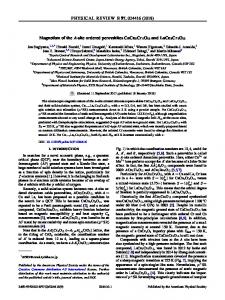
complexity of optical frequency chains (Jennings, Evenson, and Knight, 1986; Schnatz et al., 1996). Within the past 15 years, the development of the optical frequency comb has made optical frequency measurement relatively straightforward (Reichert et al., 1999; Diddams et al., 2000; Jones et al., 2000; Udem, Holzwarth, and Hänsch, 2002; Cundiff and Ye, 2003; Fortier, Jones, and Cundiff, 2003). With two of the pioneers of this technique rewarded by the 2005 Nobel Prize in Physics (Hall, 2006; Hänsch, 2006), these optical measurements are now made regularly with amazing precision in laboratories around the world. Furthermore, these optical combs have demonstrated the ability to phase coherently distribute an optical frequency throughout the optical spectrum and even to the microwave domain. The optical frequency comb outputs laser pulses with temporal widths at the femtosecond time scale and with a repetition rate of millions or billions of pulses per second. The advent of few-cycle lasers with a few femtosecond pulse width, where an ultrafast Kerr-lens mode-locking mechanism ensures phase locking of all modes in the spectrum, along with the spectral broadening via microstructured fibers, have greatly facilitated the development of wide bandwidth optical frequency combs and their phase stabilization. As in Fig. 1, the frequency and phase properties of this pulse train are given by 2 degrees of freedom: the relative phase between the carrier wave and the pulse envelope (known as the carrier-envelope offset), and the pulse repetition rate. Applying a Fourier transform to this pulse train, the laser output consists of a comb of many single-frequency modes. The mode spacing is given by the laser repetition rate, and the spectral range covered by the frequency comb is related to the temporal width of each pulse. The frequency of each comb mode is given as a multiple of the mode spacing (frep ) plus a frequency offset (f CEO ) which is related to the carrier-envelope phase offset (Telle et al., 1999; Udem et al., 1999; Jones et al., 2000). Control of these two rf frequencies yields control over the frequency of every comb mode (Ye, Hall, and Diddams, 2000; Udem, Holzwarth, and Hänsch, 2002; Ma et al., 2004). If these frequencies are stabilized to an accurate reference (caesium), the optical frequency of a cw laser or optical frequency standard can be determined by measuring the heteroydne beat between the comb and optical standard. A coarse, independent measurement of the unknown laser frequency using a commercially available wavelength meter allows one to determine which comb mode N makes the heterodyne beat with the laser. The laser frequency is then straightforwardly determined by νlaser ¼ Nfrep þ fCEO fbeat, where fbeat is the measured heterodyne beat frequency and the is determined by whether the comb mode or the unknown laser is at higher frequency. In this way, optical standards can be measured against caesium microwave standards. Furthermore, by stabilizing the comb frequency directly to an optical standard, the comb allows direct comparison of optical standards at different frequencies within the spectral coverage of the comb (Schibli et al., 2008; Nicolodi et al., 2014). These measurements can be made at the stability of the optical standards themselves, without being limited by the lower stability of most microwave standards. The femtosecond comb, using now standard laboratory techniques, thus enables microwave-to-optical, optical-to-microwave,

646


a laser source whose output frequency is stabilized to the atomic signal. A further common feature of these standards is that the requirements of initial cooling and state preparation of the atoms lead to an operation in a cyclic sequence of interrogations and measurements. This is in contrast to established atomic clocks like caesium clocks with a thermal atomic beam and hydrogen masers that provide a continuous signal. In the optical frequency standard, the laser has to serve as a flywheel that bridges the intervals when no frequency or phase comparison with the atoms is possible. Its intrinsic frequency stability, the method for interrogating the atoms, and the use of the atomic signal for the frequency stabilization need to be considered together in the overall system design of the frequency standard. In this section we discuss generic features of the methods and techniques that are applied for these purposes. A. Clock cycles and interrogation schemes

FIG. 1 (color online). (a) In the time domain, the laser output generates femtosecond pulse-width envelopes separated in time by 1=f rep. Another important degree of freedom is the phase difference between the envelope maximum and the underlying electric field oscillating at the carrier optical frequency. (b) By Fourier transformation to the frequency domain, the corresponding frequency comb spectrum is revealed. Each tooth in the comb, a particular single-frequency mode, is separated from its neighbor by f rep. The relative carrier-envelope phase in the time domain is related to the offset frequency f CEO in the frequency domain. fCEO is given by the frequency of one mode of the comb (e.g., νn ) modulo frep , and can be measured and stabilized with a f-2f interferometer. In this interferometer, one comb mode νn is frequency doubled and heterodyne beat with the comb mode at twice the frequency ν2n. Thus, by stabilizing fCEO and f rep to a well-known frequency reference, each comb mode frequency is well known. Measurement of the frequency of a poorly known optical frequency source (e.g., previously measured at the resolution of a wave meter) can be determined by measuring the heterodyne beat between the frequency source and the frequency comb.

and optical-to-optical phase-coherent measurements and distribution at a precision level often better than the atomic clocks (Ma et al., 2004, 2007; Kim et al., 2008b; Lipphardt et al., 2009; Nakajima et al., 2010; Zhang et al., 2010; Fortier et al., 2011, 2013; Hagemann et al., 2013; Inaba et al., 2013). IV. MEASUREMENT TECHNIQUES OF AN OPTICAL STANDARD

All optical frequency standards that have been realized with cooled and trapped atoms are of the passive type, i.e., the oscillator of the standard is not the atomic reference itself, but Rev. Mod. Phys., Vol. 87, No. 2, April–June 2015

The repetitive operation cycle of an optical frequency standard with cooled and trapped atoms consists of three distinct stages during which the following operations are performed: (i) cooling and state preparation, (ii) interrogation, and (iii) detection and signal processing. For a clock with neutral atoms, the first phase comprises loading of a magneto-optical trap or of an optical dipole trap from an atomic vapor or from a slow atomic beam. In the case of trapped ions, the same particles are used for many cycles, but some Doppler or sideband laser cooling is necessary to counteract heating from the interaction of the ion with fluctuating electric fields. The conditions that are applied during this trapping and cooling phase include inhomogenous magnetic fields and resonant laser radiation on dipoleallowed transitions. This leads to frequency shifts of the reference transition that cannot be tolerated during the subsequent interrogation phase. The first phase of the clock cycle is concluded with preparation of the initial lowerenergy state of the clock transition by means of optical pumping into the selected hyperfine and magnetic sublevel. Depending on the loading and cooling mechanism, this phase takes a time ranging from a few milliseconds to a few hundred milliseconds. Before starting the interrogation, all auxiliary fields that would lead to a frequency shift of the reference transition need to be extinguished. Resonant lasers that are used for cooling or optical pumping are usually blocked by mechanical shutters because the use of acousto-optic or electro-optic modulators alone does not provide the necessary extinction ratio. A time interval of a few milliseconds is typically required to ensure the reliable closing of these shutters. During the interrogation phase, radiation from the reference laser is applied to the atom. In an optimized system, the duration of this phase determines the Fourier-limited spectral resolution or line Q of the frequency standard. Provided that the duration of the interrogation is not limited by properties of the atomic system, i.e., decay of the atomic population or coherence or heating of the atomic motion, it is set to the maximum value that is possible before frequency or phase fluctuations of the reference laser start to broaden the detected line shape. For a reference laser that is stabilized to a cavity


with an instability σ y limited by thermal noise to about 5 × 10−16 around 1 s, a suitable duration of the interrogation interval is several 100 ms up to 1 s, resulting in a Fourierlimited linewidth of about 1 Hz. Referring to pioneering work on molecular beams in the 1950s (Ramsey, 1985), one distinguishes between Rabi excitation with a single laser pulse and Ramsey excitation with two pulses that are separated by a dark interval. In Ramsey spectroscopy, the two levels connected by the reference transition are brought into a coherent superposition by the first excitation pulse and the atomic coherence is then allowed to evolve freely. After the second excitation pulse the population in one of the levels is detected, which shows the effect of the interference of the second pulse with the timeevolved superposition state. Assuming that the total pulse area is set to π on resonance, Rabi excitation possesses the advantage of working with lower laser intensity, leading to less light shift during the excitation. Ramsey excitation, on the other hand, provides a narrower Fourier-limited linewidth for the same interrogation time. If the duration of the excitation pulses is much shorter than the dark interval, Ramsey excitation keeps the atoms in a coherent superposition of ground and excited states that is most sensitive to laser phase fluctuations—with the Bloch vector precessing in the equatorial plane—for a longer fraction of the interrogation time than Rabi excitation. Generalizations of the Ramsey scheme with additional pulses permit one to reduce shifts and broadening due to inhomogeneous excitation conditions or shifts that are a result of the excitation itself. An “echo” π pulse during the dark period may be used to rephase an ensemble of atoms that undergoes inhomogoenous dephasing (Warren and Zewail, 1983). An example of such an excitation-related shift is the light shift and its influence may readily be observed in the spectrum obtained with Ramsey excitation (Hollberg and Hall, 1984): The position and shape of the envelope reflects the excitation spectrum resulting from one of the pulses, whereas the Ramsey fringes result from coherent excitation with both pulses and the intermediate dark period. The fringes are less shifted than the envelope, because their shift is determined by the time average of the intensity. A sequence of three excitation pulses with suitably selected frequency and phase steps can be used to cancel the light shift and to efficiently suppress the sensitivity of the spectroscopic signal to variations of the probe light intensity (Zanon-Willette et al., 2006; Yudin et al., 2010; Huntemann, Lipphardt et al., 2012; Zanon-Willette et al., 2014). While Rabi excitation is often used in optical frequency standards because of its experimental simplicity, these examples show that the greater flexibility of Ramsey excitation may provide specific benefits. After the application of the reference laser pulses, the clock cycle is concluded by the detection phase. In most cases, the atomic population after an excitation attempt is determined by applying laser radiation to induce resonance fluorescence on a transition that shares the lower state with the reference transition. This scheme was proposed by Dehmelt and is sometimes called electron shelving (Dehmelt, 1982). In the single-ion case, the absence of fluorescence indicates population of the upper state and the presence of fluorescence population of the lower state. The method implies an efficient Rev. Mod. Phys., Vol. 87, No. 2, April–June 2015

647

quantum amplification mechanism, where the absorption of a single photon can be readout as an absence of many fluorescence photons. It is therefore also advantageously used for large atomic ensembles. If the number of photons detected from each atom is significantly greater than 1, photon shot noise becomes negligible in comparison to the atomic projection noise. A disadvantage of the scattering of multiple fluorescence photons is that it destroys the induced coherence on the reference transition and that it even expels trapped neutral atoms from an optical lattice. In a lattice clock this makes it necessary to reload the trap with atoms for each cycle. Since the loading and cooling phase takes a significant fraction of the total cycle time, reusing the same cold atoms would permit a faster sequence of interrogations, thereby improving the frequency stability. This can be realized in a nondestructive measurement that detects the atomic state not via absorption but via dispersion as a phase shift induced on a weak offresonant laser beam (Lodewyck, Westergaard, and Lemonde, 2009). If in addition to observing the same atoms, as is the case with trapped ions, the internal coherence could also be maintained from one interrogation cycle to the next, a gain in stability can be obtained. If the atomic phase can be monitored over many cycles without destroying it, the frequency instability would average with σ y ∝ τ−1 like for white phase noise, instead of σ y ∝ τ−1=2 as for white frequency noise in a conventional atomic clock. Such an atomic phase lock has been analyzed and an experimental realization proposed based on a measurement of Faraday rotation with trapped ions (Shiga and Takeuchi, 2012; Vanderbruggen et al., 2013) and for a dispersive interaction in a generic clock (Borregaard and Sørensen, 2013b). B. Atomic noise processes

In the atomic population measurement described previously, noise may arise from fluctuations in the absolute atom number N and in the atomic population distribution. For the frequency standards with cold trapped ions, N is unity or a small number that is controlled in the beginning of each cycle, so that fluctuations are eliminated. If new atoms are loaded for each cycle from a reservoir, one may expect relative variations in the atom number δN. Since fluorescence detection permits one to measure the atom number in each cycle, however, signals may be normalized to the atom number, so that the contribution from atom number fluctuations to the instability of the frequency standard scales as

1 2δN 2 þ 2 Nnph N

1=2 ;

where the first term accounts for shot noise during detection of nph photons and the second term accounts for fluctuations in the atom number between cycles (Santarelli et al., 1999). Sometimes the most severe noise contribution comes from quantum noise in the state measurement: physical measurement of a quantum system can be modeled by a Hermitian operator acting on the wave function of the system being measured, and the result of that measurement is an eigenvalue of the operator. Thus, measurement of a superposition of

648


eigenstates yields one of the corresponding eigenvalues, a statistical outcome given by the superposed weighting of the eigenstates. This implies measurement fluctuation as the wave function collapses into a projection along a particular eigenbasis. We consider the simple case of a single ion. The two levels that are connected by the reference transition are denoted as j1i and j2i and it is assumed that the ion is initially prepared in the lower state j1i. After an excitation attempt the ion generally will be in a superposition state αj1i þ βj2i and the measurement with the electron-shelving scheme is equivalent to determining the eigenvalue P of the projection operator Pˆ ¼ j2ih2j. If no fluorescence is observed (the probability for this outcome being p ¼ jβj2 ) the previous excitation attempt is regarded as successful (P ¼ 1), whereas the observation of fluorescence indicates that the excited state was not populated (P ¼ 0). In one measurement cycle only one binary unit of spectroscopic information is obtained. Under conditions where the average excitation probability p is 0.5, the result of a sequence of cycles is a random sequence of zeros and ones and the uncertainty in a prediction on the outcome of the next cycle is always maximal. These population fluctuations and their relevance in atomic frequency standards were first discussed by Itano et al. (1993), who named the phenomenon quantum projection noise (QPN). A simple calculation shows that the variance of the projection operator is given by ˆ 2 ¼ pð1 − pÞ: ðΔPÞ

ð11Þ

For N uncorrelated atoms, the variance is N times bigger. For atoms with correlated state vectors, so-called spin-squeezed states (Wineland et al., 1992), the variance can be smaller than this value, allowing for frequency measurements with improved stability (Bollinger et al., 1996); see Sec. VII.F. In the servo loop of an atomic clock, quantum projection appears as white frequency noise, leading to an instability as given in Eq. (4), and decreasing with the averaging time like σ y ∝ τ−1=2 . It imposes the long-term quantum noise limit of the clock that can be reached if an oscillator of sufficient shortterm stability, i.e., below the quantum projection noise limit for up to a few cycle times, is stabilized to the atomic signal. C. Laser stabilization to the atomic resonance

In an optical clock the frequency of the reference laser needs to be stabilized to the atomic reference transition. In most cases, the error signal for the frequency lock is derived by modulating the laser frequency around the atomic resonance and by measuring the resulting modulation of the frequency-dependent excitation probability p to the upper atomic level. With a cyclic operation imposed already by the requirements of laser cooling and state preparation, the frequency modulation may be realized conveniently by interrogating the atoms with alternating detuning below and above resonance in subsequent cycles. The value of the detuning will be chosen in order to obtain the maximum slope of the excitation spectrum and is typically close to the half linewidth of the atomic resonance. Suppose the laser oscillates at a frequency f, close to the center of the reference line. A sequence of 2z cycles is Rev. Mod. Phys., Vol. 87, No. 2, April–June 2015

performed in which the atoms are interrogated alternately at the frequency fþ ¼ f þ δm and at f − ¼ f − δm . The sum of the excited-state populations is recorded as Pþ at fþ and P− at f − . After an averaging interval of 2z cycles an error signal is calculated as e ¼ δm

Pþ − P− ; z

ð12Þ

and a frequency correction ge is applied to the laser frequency before the next averaging interval is started: f → f þ ge:

ð13Þ

The factor g determines the dynamical response of the servo system and can be regarded as the servo gain. Since the frequency correction is added to the previous laser frequency, this scheme realizes an integrating servo loop (Bernard, Marmet, and Madej, 1998; Barwood et al., 2001; Peik, Schneider, and Tamm, 2006). The time constant and the stability of the servo system are determined by the choice of the parameters g and z. If the laser frequency f is initially one-half linewidth below the atomic resonance and if pmax ¼ 1, the resulting value of ðPþ − P− Þ=z will also be close to 1. Consequently, with g ≈ 1, the laser frequency will be corrected in a single step. If g ≪ 1, approximately 1=g averaging intervals will be required to bring the frequency close to the atomic resonance and the demands on the short-term stability of the probe laser become more stringent. For g ≈ 1 and a small value of z, the short-term stability of the system may be unnecessarily degraded by strong fluctuations in the error signal because of quantum projection noise, especially if only a single ion is interrogated. For g ≈ 2, one expects unstable servo behavior with the laser frequency jumping between −δm and þδm . A servo error may occur if the probe laser frequency is subject to drift, as it is commonly the case if the short-term frequency stability is derived from a Fabry-Pérot cavity which is made from material that shows aging or in the presence of slow temperature fluctuations. Laser frequency drift rates jdf=dtj in the range from mHz=s up to Hz=s are typically observed. For a first-order integrating servo with time constant tservo , an average drift-induced error e¯ ¼ tservo df=dt is expected as the result of a constant linear drift. Since the minimally achievable servo time constant has to exceed several cycle times for stable operation, such a drift-induced error may not be tolerable. An efficient reduction of this servo error is obtained with the use of a second-order integrating servo algorithm (Peik, Schneider, and Tamm, 2006), where a drift correction edr is added to the laser frequency in regular time intervals tdr tdr

f → f þ edr :

ð14Þ

The drift correction is calculated from the integration of the error signal Eq. (12) over a longer time interval T dr ≫ tdr :

Ludlow et al.: Optical atomic clocks T dr

edr → edr þ k

X e;

ð15Þ

T dr

where the two gain coefficients are related by k ≪ g. In the case of Ramsey excitation, an error signal may also be obtained by alternately applying phase steps of π=2 to one of the excitation pulses while keeping the excitation frequency constant (Ramsey, 1985; Letchumanan et al., 2004; Huntemann, Lipphardt et al., 2012). Whether a more precise lock is achieved with stepwise frequency or phase modulation depends on specific experimental conditions: While the former is more sensitive to asymmetry in the line shape or a correlated power modulation, the latter requires precise control of the size of the applied phase steps. Because of the time needed for preparation and readout of the atoms, a dead time is introduced into each cycle during which the oscillator frequency or phase cannot be compared to the atoms. As first pointed out by Dick (1987) and Dick et al. (1990), this dead time will lead to degraded long-term stability of the standard because of downconversion of frequency noise of the interrogation oscillator at Fourier frequencies near the harmonics of the inverse cycle time 1=tc . The impact of the effect on clock stability depends on the fraction of dead time, the interrogation method (Rabi or Ramsey), and the noise spectrum of the laser (Dick, 1987; Santarelli et al., 1998): 1 σ y ðτÞ ¼ f0

sffiffiffiffiffiffiffiffiffiffiffiffiffiffiffiffiffiffiffiffiffiffiffiffiffiffiffiffiffiffiffiffiffiffiffiffiffiffiffiffiffiffiffiffiffiffiffiffiffiffiffiffiffiffiffi ffi ∞ 2 gc;m g2s;m 1X m : þ 2 Sf τ m¼1 g20 Tc g0

ð16Þ

Here Sf ðm=T c Þ is the one-sided frequency noise power spectral density of the free running probe laser (local oscillator) at the Fourier frequency m=T c, where m is a positive integer. The factors gc;m and gs;m correspond to the Fourier cosine and sine series coefficients giving the sensitivity spectral content at f ¼ m=T c (Santarelli et al., 1998) and contain the physics of the atom laser interaction. For the case of Ramsey excitation one finds (Santarelli et al., 1998) rffiffiffiffi σ yosc sinðπt=tc Þ tc σ y lim ðTÞ ≈ pffiffiffiffiffiffiffiffiffiffiffi ; 2 ln 2 πt=tc T

ð17Þ

where σ yosc is the flicker floor instability of the oscillator. With achieved experimental parameters like t=tc > 0.6 and a flicker floor σ yosc < 5 × 10−16 (Kessler et al., 2012), it can be seen thatpthe ffiffiffiffiffiffiffiffiffi limitation from the Dick effect σ y lim ≈ 2 × 10−16 tc =T is well below the quantum projection noise limited instability for single-ion clocks, but may impose a limit on the potentially much lower instability of neutral atom lattice clocks. For the frequency comparison between two atomic samples, the Dick effect may be suppressed by synchronous interrogation with the same laser (Chou et al., 2011; Takamoto, Takano, and Katori, 2011; Nicholson et al., 2012), whereas for improved stability of the clock frequency, a single oscillator may be locked to two atomic ensembles in an interleaved, dead-time free interrogation (Dick et al., 1990; Biedermann et al., 2013; Hinkley et al., 2013). Rev. Mod. Phys., Vol. 87, No. 2, April–June 2015

649

V. TRAPPED-ION OPTICAL FREQUENCY STANDARDS

The invention of electromagnetic traps for charged particles by Paul and Dehmelt in the 1950s marked an important step toward realizing the ideal environment for precision spectroscopy: an unperturbed system with long trapping times. Ion traps have played an important role in spectroscopy and precision measurements ever since, which was recognized by awarding the 1989 Nobel Prize in Physics to Dehmelt, Paul, and Ramsey (Dehmelt, 1990; Paul, 1990; Ramsey, 1990). The absence of a magnetic field made Paul traps the preferred choice over Penning traps for frequency standards, thus avoiding undesired internal level shifts through the Zeeman effect. The basic principle behind the simplest form of a threedimensional Paul trap is a time-varying electric quadrupole potential in which the balance between the Coulomb force and the inertia of the ions keeps the ions trapped (Straubel, 1955; Paul, Osberghaus, and Fischer, 1958; Paul, 1990). The traps typically provide several electron volt deep potentials, offering trap lifetimes that are limited by (photo-)chemical reactions with background gas atoms and range from several hours to months, depending on the atomic species and the background gas pressure. In spherical 3D Paul traps, only a single ion can be trapped at zero field. Linear Paul traps allow storage of strings of ions (Raizen et al., 1992), potentially allowing an improvement in clock stability by interrogating several ions at once (Herschbach et al., 2012; Pyka et al., 2014). However, achieving the zero-field condition for many ions is a technological challenge. As a consequence, all optical single-ion frequency standards implemented up to now trade stability for accuracy and use a single clock ion. The idea of using trapped ions as optical frequency references dates back to Dehmelt (1973), who proposed several species and experimental implementations (Dehmelt and Toschek, 1975; Dehmelt and Walther, 1975), including the electron-shelving technique (Dehmelt, 1975). Doppler or sideband laser cooling (Hänsch and Schawlow, 1975; Wineland and Dehmelt, 1975; Neuhauser et al., 1978a, 1978b, 1980; Wineland, Drullinger, and Walls, 1978; Wineland and Itano, 1981) localizes the ion in a few 10 nm large wave packet around the zero point of the field. This strong localization in a nearly trapping-field-free environment allows spectroscopy in the recoil-free Lamb-Dicke regime (Dicke, 1953). The experimental realization of Dehmelt’s electron-shelving state detection technique by observing quantum jumps in Baþ (Nagourney, Sandberg, and Dehmelt, 1986; Sauter et al., 1986) and Hgþ (Bergquist et al., 1986) was an important prerequisite for spectroscopy of few particle systems with high signal-to-noise ratio. High resolution optical spectroscopy of trapped ions was first accomplished by optical two-photon excitation on the dipole-forbidden S-D transition in a cloud of Hgþ ions (Bergquist et al., 1985) and by direct laser excitation on a single Hgþ ion (Bergquist, Itano, and Wineland, 1987), laying the foundation for the development of optical ion clocks. There are a number of excellent previous reviews on trapped ions and applications to microwave spectroscopy (Dehmelt, 1968, 1969; Wineland, Itano, and Van Dyck, Jr., 1983; Blatt, Gill, and Thompson, 1992; Fisk, 1997), early optical spectroscopy (Dehmelt, 1981, 1982), and optical

650


frequency standards (Madej and Bernard, 2001; Riehle, 2004; Hollberg, Oates et al., 2005; Maleki, 2008; Margolis, 2009; Gill, 2011; Poli et al., 2013). In the following, we discuss the principles and operation of trapped-ion optical frequency standards and focus on the features and limitations of some of the most developed systems.

achieved by choosing Ωrf ≫ ωj , the micromotion amplitude is smaller by an order of magnitude compared to the amplitude of secular motion uj . In this regime time scales separate and the effects of micromotion can be largely neglected. The dynamic and static trapping potentials can be approximated by a harmonic pseudopotential of the form (Dehmelt, 1968) ΦP ð~rÞ ¼

A. Trapping ions

According to Earnshaw’s theorem, stable trapping of charged particles in free space using only dc fields is not possible. This is a direct consequence of the Laplace equation for electrostatic fields. Oscillating electromagnetic fields provide a way around this fundamental limitation. The Paul trap (Paul, Osberghaus, and Fischer, 1958; Fischer, 1959; Paul, 1990) is a prime example for the realization of such a trap. It employs an oscillating quadrupole potential, resulting in stable confinement of a charged particle for certain operation parameters (McLachlan, 1947; Meixner and Schäfke, 1954; Ghosh, 1995). In the most general case, we consider a superposition of a static quadrupole and an ac electric quadrupole potential oscillating at an angular frequency Ωrf . The electric fields are generated by two sets of electrodes with characteristic length scales Rdc and Rrf and applied voltages V dc and V rf , generating the dc and ac potentials, respectively. The total potential can then be written as αx x2 þ αy y2 þ αz z2 ϕð~r; tÞ ¼ V dc 2Rdc 2 þ V rf cos Ωrf t

α~ x x2 þ α~ y y2 þ α~ z z2 ; 2Rrf 2

ð18Þ

with parameters κ, αj , and α~ j that are determined by the electrode geometry. Laplace’s equation Δϕð~r; tÞ ¼ 0 imposes the relations X j¼x;y;z

αj ¼ 0

and

X

α~ j ¼ 0

ð19Þ

j¼x;y;z

between the geometrical factors. For spherical Paul traps, αx ¼ αy ¼ −ð1=2Þαz and α~ x ¼ α~ y ¼ −ð1=2Þα~ z . Threedimensional confinement of the charged particle is achieved solely through dynamical electric forces. Implementations of these types of traps are discussed in Sec. V.A.1. Another popular choice of the geometry parameters is αx ¼ αy ¼ −ð1=2Þαz and α~ x ¼ −α~ y , α~ z ¼ 0, corresponding to a linear Paul trap, discussed in Sec. V.A.2. Radial (x; y) confinement is provided by the two-dimensional dynamical quadrupole potential, whereas axial (z) trapping is achieved through a three-dimensional static quadrupole potential. Deviations from the cylindrical symmetry can be described by αx ≠ αy and α~ x ≠ α~ y , while maintaining Eqs. (19). In this trapping potential, the ion performs slow harmonic oscillations with secular frequencies ωj and a superimposed micromotion oscillation at the trap drive frequency. Micromotion is intrinsic to the trapping concept and thus unavoidable. Under stable trapping conditions, typically Rev. Mod. Phys., Vol. 87, No. 2, April–June 2015

1X 2 2 mωj uj : 2 j

ð20Þ

The trap frequencies are given by sffiffiffiffiffiffiffiffiffiffiffiffiffiffiffiffiffiffiffiffiffiffiffiffiffiffiffiffiffiffiffiffiffiffiffiffiffiffiffiffiffiffiffiffiffi Q2 α~ 2j V 2ac Qαj V dc ; ωj ≈ þ 2 mRdc 2Ωrf 2 m2 Rrf 4

ð21Þ

which are typically on the order of a few 100 kHz to a few MHz in traps for optical clocks. In optical clocks, second-order Doppler shifts from residual motion as further discussed in Sec. V.C.1 are significantly reduced through laser cooling of the trapped ion (Wineland, Itano et al., 1987). Doppler cooling typically reduces the temperature of a single trapped ion to below mK temperatures, corresponding to a motional amplitude of rffiffiffiffiffiffiffiffiffi kB T uj ∼ ∼ 70 nm mω2 for a single Caþ ion in a trap of 1 MHz trap frequency. This illustrates the fact that the ion is very well localized and probes only the very bottom of the trap, where it is harmonic. In the derivation of Eq. (18), we implicitly assumed that the symmetry axis for the dc and ac electrodes coincides. In principle, this can be achieved through precision machining of the electrodes and by nulling any external dc or ac electric field that pushes the ion away from the trap center. In practice, however, machining tolerances and insufficiently compensated stray fields push the ion into the rf trapping field, causing so-called excess micromotion (Berkeland et al., 1998b). Stray fields are believed to arise from patch charges on the electrodes and insulators, generated by contact potentials or charge buildup from ionization via electron bombardment during loading, or through the photoeffect from UV lasers (Harlander et al., 2010). Patch fields can be nulled through additional compensation electrodes. However, they tend to fluctuate on slow time scales and need to be compensated from time to time (Tamm et al., 2009). There are several techniques for micromotion compensation. The simplest technique is based on the observation of the ion’s position as the trapping conditions are changed: If patch fields are compensated, the ion does not move as the rf potential is lowered. In the nonresolved-sideband regime, a phase-synchronous detection of fluorescence photons with the trap rf exhibits a modulation as a function of the relative phase in the presence of micromotion (Blümel et al., 1989; Berkeland et al., 1998b). In the resolved-sideband regime, the Rabi frequency of a micromotion sideband of the clock transition scales with the modulation index of the excess micromotion (Leibfried et al., 2003). A fourth technique uses parametric heating of the secular motion through amplitude modulation of the trap rf at


the secular motional frequencies (Ibaraki, Tanaka, and Urabe, 2011; Narayanan et al., 2011). All techniques require probing the ion’s micromotion along three noncoplanar directions. For two-ion crystals with ions having a different mass, the radial confinement of the two ions differs. Radial stray electric fields therefore result in a tilting of the ion crystals’ symmetry axis with respect to the trap axis. As a consequence, radial and axial two-ion modes become coupled, which leads to additional motional sidebands when probing the excitation spectrum in the resolved-sideband regime along the trap axis. Nulling of these sidebands provides another means for micromotion compensation (Barrett et al., 2003). The choice of optimum trap electrode and support structure materials depends on a number of technical and practical considerations, as well as the dominant systematic shifts of the considered clock ion species. A careful calibration of the blackbody radiation shift requires precise knowledge of the effective temperature seen by the ion. This is most easily achieved for ion traps at a homogeneous and well-defined temperature. Ohmic heating of the electrodes can be prevented by using a nonmagnetic, high-conductivity metal, such as gold. Similarly, the mounting structure of the electrodes should be made from a dielectric material with a small rf loss tangent at the typical rf drive frequencies of 10–100 MHz. At the same time, the material should have a high thermal conductivity to ensure a homogeneous temperature. Materials fulfilling these conditions include diamond, sapphire (Al2 O3 crystal), alumina (Al2 O3 ceramics), aluminum nitride (AlN ceramics), and to a lesser extent fused silica. Another aspect concerns heating of the ions in the trap during interrogation, which increases the uncertainties in temperature-related shifts, such as the second-order Doppler shift. Motional heating arises through electric field noise at the secular frequencies of the ion (Wineland et al., 1998; Turchette et al., 2000). Depending on the particular trap implementation there can be many origins for such heating, ranging from Johnson noise of drive and filter electronics to electrode surface contaminants, which are reviewed in detail by Brownnutt et al. (2014).

651

1. Paul traps

Figure 2(a) shows the geometry studied by Paul and coworkers (Paul, Osberghaus, and Fischer, 1958; Fischer, 1959; Paul, 1990). It consists of cylindrically symmetric ring and end cap electrodes between which a dc and an ac voltage V dc and V rf , respectively, are applied. The hyperbolic shape of the electrodes ensures a dominant quadrupole potential, even very close to the electrodes. However, the Paul trap offers only restricted optical access for laser cooling, clock interrogation, and fluorescence detection. Beaty (1987) introduced a quadrupole geometry with conical electrodes featuring larger optical access [see Figs. 2(b) and 2(c)]. This type of trap is used for the Ybþ and Hgþ ion clocks at Physikalisch-Technische Bundesanstalt (PTB) and the National Institute of Standards and Technology (NIST), respectively. A stronger variation of the original Paul design in which the end cap electrodes are pulled away from the ring was introduced by Straubel (1955). It also offers larger optical access and can be implemented in several variations (Yu, Dehmelt, and Nagourney, 1989; Yu, Nagourney, and Dehmelt, 1991; Schrama et al., 1993). An even more open geometry with good approximation of quadrupole potential is obtained with the end cap trap (Schrama et al., 1993), where the ring is replaced by two cylindrical shields that surround the rfcarrying end cap electrodes [see Fig. 2(d)]. This geometry is employed in the Srþ ion clocks at the National Physical Laboratory (NPL) (Margolis et al., 2004) and the National Research Council Canada (NRC) (Dubé et al., 2010; Madej et al., 2012). Typical trap frequencies in all ion clock experiments are on the order of a few megahertz in all directions. 2. Linear ion traps

In many applications it is desirable to trap more than one ion in a micromotion-free configuration (Raizen et al., 1992). It is an important requirement for implementing quantum logic spectroscopy (see Sec. V.E) and scaling single-ion to multi-ion optical clocks for improved stability

FIG. 2 (color online). Electrode configurations for spherical Paul traps. (a) Cut through the cylindrically symmetric electrode geometry

used by Paul. The oscillating potential U rf ¼ V rf cos Ωrf t is applied between the ring and the end cap electrodes. (b) Paul trap used for the Ybþ frequency standard at PTB. From Tamm, Engelke, and Bühner, 2000. (c) Paul trap used for the Hgþ frequency standard at NIST. From Oskay, Itano, and Bergquist, 2005. (d) End cap trap. From Schrama et al., 1993. The inner end caps are 0.5 mm in diameter and are separated by 0.56 mm. The oscillating potential U rf is applied to the inner end cap electrodes. The outer electrodes (outer diameter 2 mm) are normally grounded; however, if required small potentials can be applied to compensate micromotion in the axial direction. Rev. Mod. Phys., Vol. 87, No. 2, April–June 2015

652


(Prestage et al., 1990; Herschbach et al., 2012). Linear Paul traps provide such a micromotion-free environment along the zero line of the rf electric field if the radial confinement is much stronger than the axial. Their design is derived from the quadrupole mass filter (Paul and Raether, 1955; Drees and Paul, 1964), which provides radial confinement through an oscillating 2D quadrupole potential. Trapping in all three dimensions is accomplished by superimposing a 3D static quadrupole field, providing mostly axial confinement (Raizen et al., 1992). This field configuration can be implemented through a variety of electrode geometries. Figure 3 shows two designs employed for the Caþ (Chwalla et al., 2009) and Alþ (Rosenband et al., 2007) optical frequency standards. The Innsbruck design uses four symmetrically arranged blade electrodes with an electrode-electrode distance of 1.6 mm to which an rf voltage of ∼1 kV at a frequency of around 25 MHz is applied to create the 2D rf quadrupole. Two tip electrodes separated by 5 mm to which a positive dc voltage of around 2 kV is applied provide axial confinement (Gulde, 2003). The electrodes are made from nonmagnetic steel, whereas the ceramic support is made from Macor. When this trap is operated with two of the rf electrodes connected to ground (asymmetric driving), axial micromotion arises from a distortion of the 2D quadrupole, since the tip electrodes act as rf ground, thus removing the radial symmetry. This effect can be circumvented by applying either additional rf to the tip electrodes or rf voltages oscillating around rf ground, to all four rf electrodes (symmetric driving). The first generation NIST trap for Alþ is made from laserstructured and gold-coated alumina wafers, separated by 440 μm (Rowe et al., 2002). This microstructured approach allows for high accuracy in the electrode geometry and provides a path for scalable quantum information processing

(Kielpinski, Monroe, and Wineland, 2002). An rf voltage of around 250 V and a dc voltage of up to 12 V results in secular frequencies of a single Beþ ion of 8 MHz radially and 5 MHz axially. The second NIST trap for Alþ uses segmented goldcoated beryllium-copper electrodes, resembling the electrode geometry of the first generation NIST trap, but using conventional machining and larger dimensions (0.4 mm distance between ion and nearest electrode) with the goal of reducing micromotion and motional heating from fluctuating patch potentials (Chou, Hume, Koelemeij, et al., 2010). The bladeshaped electrodes are mounted onto and indexed to alumina rods that are mounted into a precision machined metal cage. A linear trap geometry for multi-ion optical clocks has been designed that combines the precision of laser-machined wafers with large trap geometries for low motional heating rates and excellent laser access (Herschbach et al., 2012). High symmetry of the electrode geometry (e.g., by adding slots to the rf electrodes to match the gaps between dc segments) combined with integrated compensation electrodes allows storing tens of ions in a trap with small excess micromotion (Herschbach et al., 2012; Pyka et al., 2014). When two or more ions are stored in a linear Paul trap, their motion becomes strongly coupled and a normal mode description for the motion of the ions around their equilibrium position applies (Wineland, Bergquist et al., 1987; James, 1998; Kielpinski et al., 2000; Morigi and Walther, 2001). Each normal mode is associated with a mode frequency and motional amplitudes for the ions. For a two-ion crystal with a large mass ratio, the mode amplitudes differ significantly. The Doppler cooling rate scales with the motional amplitude. When cooling only on one of the ions, as is the case in the Alþ clock, additional motional heating can thus result in an elevated temperature of weakly cooled modes (Wübbena et al., 2012).

Linear ion-trap electrode geometries. (a) The Innsbruck trap geometry [upper panel (Gulde, 2003)] is implemented using elongated blades for the rf and two conical tips for the dc electrodes (lower panel). (b) The NIST trap geometry [upper panel (Rowe et al., 2002)] is implemented using microstructured segmented electrodes (lower panel). This allows splitting the tip electrodes and moving them away from the axial symmetry line, enabling improved laser access. Unsegmented electrodes are connected to rf potential V rf cos Ωrf t, outer-segment electrodes are at a positive dc potential V dc , and inner-segment electrodes are at ground. FIG. 3 (color online).



B. Cooling techniques and Lamb-Dicke regime

Techniques to suppress motion-induced frequency shifts have long played a central role in optical spectroscopy. Doppler laser cooling (Hänsch and Schawlow, 1975; Wineland and Dehmelt, 1975; Neuhauser et al., 1978a, 1978b, 1980; Wineland, Drullinger, and Walls, 1978; Wineland and Itano, 1981; Stenholm, 1986) on transitions with linewidth Γ achieves temperatures of TD ¼ κ

ℏΓ ; 2kB

independent of the atomic mass and the trap frequency. The parameter κ is of order unity and depends on the laser cooling geometry (Javanainen, 1980). For a few MHz broad transitions, this corresponds to temperatures in the few hundred μK regime, thus reducing second-order Doppler shifts to well below 10−17 fractional frequency uncertainty for heavy clock ion species, such as Ybþ or Srþ. In contrast to neutral atoms in free space, trapped ions require only a single cooling laser with k-vector components along all three trap axes (Wineland and Itano, 1979). However, one has to ensure that all trap frequencies are different to spatially fix the normal mode axes to the geometry of the trap (Itano and Wineland, 1982). The megahertz fast oscillations of the ion(s) in the trap allow efficient cooling when the ion(s) are moving toward the laser beam. This semiclassical picture is valid if the quantized mode structure of the ion’s motion in the trap can be neglected, which is the case in the so-called weak binding regime in which the trap frequency ω is much smaller than the linewidth of the cooling transition (ω ≪ Γ) (Wineland and Itano, 1979). The situation changes when considering narrow transitions (ω ≫ Γ). In this tight binding regime motional sidebands are spectrally resolved from the carrier and can be individually addressed, resulting in a simultaneous change in the internal and motional state. In a simple picture, the spatial gradient of the laser’s electric field along its propagation direction (characterized by the wave number k) interacts with the motional wave packet of the ionpin the trap (characterized ffiffiffiffiffiffiffiffiffiffiffiffiffiffiffi by its ground-state size u0 ¼ ℏ=2mω). The parameter describing the strength of the interaction is the so-called Lamb-Dicke parameter η ¼ ku0. Absorption and emission of photons by an unbound atom are associated with photon recoil, resulting in an energy shift Erec ¼ ℏ2 k2 =2m of the observed line. For trapped ions, this recoil is suppressed if Erec =ℏω < 1, which is equivalent to η2 < 1, reminiscent of the Mössbauer effect in nuclear physics. Optical clocks based on trapped ions are typically deep in this regime, thus eliminating recoil shifts. If we restrict ourselves to a two-level system with ground (j↓i) and excited (j↑i) states coupled to a single motional mode (jni) with excitation n, the resulting system is described by a Jaynes-Cummings–type model (Wineland et al., 1998; Leibfried et al., 2003). Particularly simple expressions for the transition strengths are obtained in the Lamb-Dicke regime for which the size of the motional wave function jψ m i ffi is small compared to the wavelength p ffiffiffiffiffiffiffiffiffiffiffiffiffiffiffiffiffiffiffiffiffiffiffiffiffiffiffi hψ m jk2 uˆ 2 jψ m i ≪ 1. In this case three distinct transitions are dominant: (i) Carrier (CAR) transitions with Rabi frequency Ω change only the electronic state (j↓ijni ↔ j↑ijni); Rev. Mod. Phys., Vol. 87, No. 2, April–June 2015

653

pffiffiffi (ii) red sideband (RSB) transitions with Rabi frequency ηΩ n excite the electronic state and remove a quantum of motion (j↓ijni ↔ j↑ijn − 1i); (iii) blue sideband (BSB) transitions pffiffiffiffiffiffiffiffiffiffiffi with Rabi frequency ηΩ n þ 1 excite the electronic state and add a quantum of motion (j↓ijni ↔ j↑ijn þ 1i). Outside the Lamb-Dicke limit, terms of higher order in the Lamb-Dicke factor need to be considered, changing the Rabi frequencies of the transitions (Wineland and Itano, 1979; Wineland et al., 1998) and allowing higher-order motional transitions. In the tight binding regime, the kinetic energy of the ion can be further reduced through resolved-sideband cooling (Wineland and Dehmelt, 1975; Dehmelt, 1976). By continuously driving the first red sideband transition motional energy is removed and dissipated through spontaneous emission from the excited state. The latter step involves scattering of a photon, which provides the required dissipation and is recoil free with a high probability in the Lamb-Dicke limit. Residual recoil from the dissipation step together with off-resonant excitation of CAR and BSB transitions determines the achievable average motional quantum number n¯ of n¯ ≈ Cs ðΓ=ωÞ2 ; where Cs is a numerical factor on the order of 1 depending on the selection rules of the atomic transition (Neuhauser et al., 1978a; Wineland and Itano, 1979; Stenholm, 1986; Wineland, Itano et al., 1987). Although up to now Doppler cooling for reducing second-order Doppler shifts was sufficient, future ion clocks operating at or below the 10−18 fractional frequency uncertainty may require more involved cooling techniques. In typical ion-trap experiments, the ground state can be populated with a probability reaching 99.9% (Roos et al., 1999), reducing this shift to its value in the ground state of the trap and its uncertainty to well below that. Different implementations of sideband cooling are further discussed by Eschner et al. (2003). C. Systematic frequency shifts for trapped ions

The most important systematic frequency shifts encountered in trapped-ion frequency standards are Doppler shifts resulting from the residual motion of the ion and shifts from the interaction with external electromagnetic fields. For trapped ions, there is always a connection between the Doppler and Stark shifts, because an ion with higher kinetic energy will also be exposed to higher field strength in the confining quadrupole potential of the trap. The sensitivity to field-induced shifts depends on the type of the reference transition and on properties of the specific ion. This has been an important criterion in the selection of suitable ions. In the following we expand on the main frequency shifting effects already introduced in Sec. I and discuss their specific properties in the context of trapped ions (Itano, 2000; Madej and Bernard, 2001; Madej et al., 2004; Lea, 2007; Dubé et al., 2013). 1. Motion-induced shifts

The oscillation frequencies of the ion in the trap are much higher than the linewidth of the optical reference transition. Therefore, the linear Doppler effect [first term in Eq. (10)]

654


from secular and micromotion leads to sidebands in optical excitation or emission spectra, but does not shift the carrier. However, a shift can arise from a displacement of the ion in the direction of the probe laser beam if it is correlated with the interrogation cycle or continuous over an appreciable time scale. Such an effect could be induced by electric fields correlated with the probe laser, or thermal effects changing the position between the ion trap and the reference phase of the probe laser. If the clock interrogation light is in the UV spectral regime (such as for the Alþ clock), it can eject photoelectrons when hitting a surface (Harlander et al., 2010). Depending on the geometry of the trap and laser direction, the created charges can alter the position of the ion, resulting in a linear Doppler shift. Some of these effects can be eliminated by probing the ion from two counterpropagating directions and averaging the observed transition frequencies (Rosenband et al., 2008b; Chou, Hume, Koelemeij, et al., 2010). Residual secular motion at the laser cooling limits determines the time dilation shift, which is mostly relevant for light ion species [second term in Eq. (10)]. Moreover, secular motion results in an increased size of the ion’s time-averaged wave packet, which extends into the region of a nonzero oscillating trap field. As a consequence, for typical trap operation parameters (Wineland, Itano et al., 1987; Berkeland et al., 1998a; Wübbena et al., 2012) the kinetic energy from secular motion is doubled through an equal contribution from micromotion. The total kinetic energy is thus P the sum of the secular kinetic energy Es ¼ ð1=2Þ α ℏωα ðn¯ α þ 1=2Þ and the micromotion energy Emm ≈ Eemm þ Es , containing a term from excess micromotion and secular-motion-induced micromotion. It is interesting to note that even for an ion in the ground state of the trap, the kinetic energy contribution from zero-point fluctuations result in a nonvanishing fractional time dilation shift of the order of −10−18 for Alþ in a single mode with frequency 5 MHz. 2. Zeeman effect

While a static magnetic field is not required for the operation of the Paul trap, a weak homogeneous field (typically in the range of 1 to 100 μT) is applied in order to separate the Zeeman components of the reference transition and to provide a controllable quantization axis for the interaction of the ion with the different laser fields. The methods for the control or compensation of resulting linear and quadratic Zeeman shifts are similar to those applied in other types of atomic clocks (see Sec. II.C).

While static electric stray fields can easily be diagnosed via the induced micromotion and can be nulled by compensation potentials on extra electrodes, the dynamics of the ion does not provide a similarly sensitive measure for residual field gradients and the strength and symmetry of these is initially unknown. Linear Paul traps require a static electric field gradient for closure along the trap axis. Since the gradient is related to the ion’s axial trap frequency, it can be determined with high accuracy and allows a precision measurement of the electric quadrupole moment (Roos et al., 2006). The Hamiltonian describing the interaction of an external field gradient with the atomic quadrupole moment is (Itano, 2000) HQ ¼ ∇Eð2Þ · Θð2Þ :

ð22Þ

Here ∇Eð2Þ is a symmetric traceless second-rank tensor describing the electric field gradient at the position of the ion and Θð2Þ is the electric quadrupole operator for the atom. Transforming to principal axes, the electric potential creating the gradient can be written as Φ ¼ A½ð1 þ ϵÞx02 þ ð1 − ϵÞy02 − 2z02 .

ð23Þ

Treating the quadrupole shift as a small perturbation of the Zeeman shifts in the basis of states jγJFmF i and applying the Wigner-Eckart theorem to Θð2Þ , the diagonal matrix elements of HQ can be written as HQ ¼ hγJFmF jH Q jγJFmF i ¼

ð24Þ

−2½3m2F − FðF þ 1ÞAhγJFjjΘð2Þ jjγJFi ½ð2F þ 3Þð2F þ 2Þð2F þ 1Þ2Fð2F − 1Þ1=2 × ½ð3cos2 β − 1Þ − ϵsin2 βðcos2 α − sin2 αÞ;

ð25Þ

where α; β are the first two of the Euler angles that relate the principal axis frame to the laboratory frame where the z axis is parallel to the magnetic field. The reduced matrix element of Θð2Þ in the ðIJÞ coupling scheme is ð2Þ

ðγIJF∥Θ ∥γIJFÞ ¼ ð−1Þ ×

IþJþF

ð2F þ 1Þ

J

2 J

−J

0 J

−1

J

2

J

F

I

F

Θðγ; JÞ;

ð26Þ

where Θðγ; JÞ is the quadrupole moment of the ðγ; JÞ state, which is defined as

3. Quadrupole shift

In the case of an atomic state with J > 1=2 (and F > 1=2) the electronic charge distribution can have multipole moments that couple to an external electric field gradient, giving rise to the so-called quadrupole shift of the energy level. A static electric field gradient is not required for the operation of a Paul trap, but it turns out that because of the proximity of the ion to the trap electrodes and due to the presence of patch potentials on these, the ion may be exposed to an unintentionally applied field gradient as strong as 1 V=mm2 that will lead to a level shift on the order of 1 Hz for a quadrupole moment of ea20 . Rev. Mod. Phys., Vol. 87, No. 2, April–June 2015

ð2Þ

Θðγ; JÞ ¼ hγJJjΘ0 jγJJi:

ð27Þ

Equation (25) possesses symmetry properties that can be used for a cancellation of the quadrupole shift without prior knowledge about strength or orientation of the electric field gradient. Itano (2000) showed that the sum of the angledependent factor in square brackets (a linear combination of spherical harmonics) vanishes for any three mutually perpendicular orientations of the quantization axis z. Therefore, the average of the transition frequency taken for


three mutually perpendicular orientations of a magnetic field of the same magnitude does not contain the quadrupole shift. The method has been verified experimentally and has been used in frequency standards with 87 Srþ , 171 Ybþ , and 199 Hgþ (Margolis et al., 2004; Oskay, Itano, and Bergquist, 2005; Schneider, Peik, and Tamm, 2005; Oskay et al., 2006). In a mm-size Paul trap with 171 Ybþ , stray field-induced, slowly variable quadrupole shifts of about 1 Hz have been observed over a period of 74 days after loading the ion (Tamm et al., 2009). The suppression of the quadrupole shift that can be achieved depends on the precision to which the three magnetic-field orientations are orthogonal. The uncertainty in the angles between field orientations has to be about 1° to get a suppression of the shift by a factor of 100. Such a precision and temporal stability of the magnetic field requires the use of magnetic shielding around the trap, with a set of field coils mounted inside the shield. An alternative option for the cancellation of the quadrupole shift is based on the mF dependence in Eq. (25): Because F X

½3m2 − FðF þ 1Þ ¼ 0;

ð28Þ

m¼−F

an average of the transition frequency over all Zeeman sublevels does not contain the quadrupole shift. For higher values of F it will be more efficient to measure the transition frequencies for two values of jmj and to interpolate the linear dependence of the frequency on m2 to the unperturbed value obtained at the “virtual” quantum number m20 ¼ FðF þ 1Þ=3 (Dubé et al., 2005). Depending on the quantum numbers, different interrogation sequences may be used to simultaneously suppress combinations of m-dependent shifts, like, for example, the quadrupole shift and the linear-Zeeman shift (Margolis et al., 2004; Chwalla et al., 2009; Madej et al., 2012; Dubé et al., 2013). In all the reference transitions studied today, the ground state fulfills J < 1 so that the quadrupole shift needs to be considered only for the excited-state sublevels. Unlike the method of averaging over three orientations of the quantization axis, averaging over the Zeeman components also eliminates higher orders of the quadrupole shift. In comparison to static patch fields, the oscillating quadrupole potential of the Paul trap generates much stronger field gradients on the order of 1 kV=mm2 . While the time-averaged first-order quadrupole shift produced by the oscillating field is zero, it could lead to a contribution from the second-order quadrupole shift (Cohen and Reif, 1957). 4. Stark shift

An ion in a Paul trap can be exposed to dc electric fields introducing excess micromotion and to oscillating electric fields arising from blackbody radiation, laser fields, or the rf trap potential. Exposing the atom to a nonvanishing rms electric field displaces the energy levels via the quadratic Stark effect [cf. Eq. (6)]. Comparison of the tensor part of the Stark shift with the expression for the quadrupole shift [see Eq. (25)] shows that both effects possess identical dependences on the orientation of the quantization axis and on the m numbers. Rev. Mod. Phys., Vol. 87, No. 2, April–June 2015

655

Therefore, averaging methods that suppress the quadrupole shift will also eliminate the tensorial Stark shift. Since the oscillating trapping electric field drives a motion of the ion with jEj2 ∝ jvj2 , there is a direct connection between the second-order Stark and Doppler shifts. In cases such as Caþ and Srþ , where the scalar Stark shift from the differential polarizability ΔαS increases the transition frequency, a cancellation of both shifts is obtained for a specific pffiffiffiffiffiffiffiffiffiffiffiffiffiffiffiffiffiffiffiffiffiffi value of the trap radio frequency Ωrf ¼ ðe=mcÞ ℏω0 =jΔαS j (Itano, 2000; Dubé et al., 2005, 2014; Madej et al., 2012). A dynamic Stark effect will be produced by laser light impinging on the ion and will be described by an expression like Eq. (6), where the static polarizabilities are replaced by frequency-dependent dynamic polarizabilities and the rms electric field strength hE2 i ¼ I L =cϵ0 is proportional to the laser intensity I L. The dynamic polarizability in general is composed of contributions from several dipole transitions coupling to the levels of the reference transition. In the case of a two-level system that is driven by near resonant light at Rabi frequency ΩR and detuning δ, the shift is ΔfL ¼ 2δΩ2R =ð4δ2 þ Γ2 Þ. Light from cooling and repumping lasers that couples resonantly to one of the levels of the reference transition is therefore usually blocked by mechanical shutters and care is taken to avoid the presence of stray light during the interrogation period. An exception is the quantum logic clock (see Sec. V.E), where cooling of the logic ion of a different species is continued during the clock interrogation. In the case of a strongly forbidden reference transition like the electric octupole transition in Ybþ , the light shift induced by the reference laser itself through the coupling to other levels needs to be corrected for. 5. Blackbody radiation shift

The electric field associated with thermal radiation emitted by the trap structure and the inner surface of the vacuum chamber also gives rise to a quadratic Stark shift of the reference transition, the so-called blackbody radiation shift (Itano, Lewis, and Wineland, 1982). If the thermal radiation field is isotropic, the tensor contribution to the Stark shift averages to zero. Table V lists the expected shifts at T ¼ 300 K for the most important ion reference transitions. At the present stage, the uncertainty from the blackbody radiation shift makes an important contribution to the systematic uncertainty budgets of many of the trapped-ion optical frequency standards, resulting partly from uncertainty in the polarizabilities and partly from incomplete knowledge of the radiation field. The trap structure is subject to heating through the applied radio-frequency voltage, from Ohmic losses in the conductors and from dieletric losses in the insulators. The employed materials possess very different emissivities for infrared radiation, ranging from 0.02 for a polished metal surface to 0.9 for ceramics. In an experiment with thermistors attached to different parts of an ion trap, temperature differences up to about 25 K have been observed (Dubé et al., 2013). Attempts to analyze the temperature distribution in ion traps by finite-element modeling indicate that the use of materials with low electric losses and the provision of good thermal contact to a heat sink may constrain the rise of the

656


effective radiation temperature seen by the ion due to applied rf voltages to below 1 K at room temperature. D. Ionic candidates and their electronic structure

Several different ion species have been considered for optical clocks. Each of them has advantages and disadvantages concerning systematic shifts and technical complexity. By definition, the most accurate frequency standard will be the one with the lowest uncertainties in the systematic shift evaluation. However, this does not necessarily imply that the shifts themselves are small. In fact, they can be quite large if they are known with sufficient precision. This requires a thorough investigation of all shifts and associated uncertainties. The evaluation will depend on an accurate knowledge of the atomic shift coefficients and the fluctuations in the shift inducing effects, e.g., electric and magnetic fields. Without a priori knowledge of these parameters, it is impossible to judge which species will offer the most accurate reference transition. After a brief historical review, we discuss in the following the order of magnitude of the systematic shifts introduced in Sec. V.C, concentrating on ion species that have been brought to a sufficiently high level of accuracy to allow a comparison of each species’ pros and cons. The discussion is complemented by Table I which provides a detailed list of atomic coefficients for each species. The ideal optical clock ion species has a clock transition with a high-Q factor that is insensitive to external field perturbations and auxiliary transitions for laser cooling, state preparation through optical pumping, and internal state detection. Historically, the first proposals for a single-ion optical clock by Dehmelt (1973, 1975) and Wineland and Dehmelt (1975) were based on Tlþ , since the comparatively short excited clock state lifetime of 50 ms seemed to allow fluorescence detection and laser cooling directly on the clock transition. However, a Tlþ clock was never realized. The invention of the electron-shelving technique for internal state detection (Dehmelt, 1975) and laser cooling on fast transitions (Hänsch and Schawlow, 1975; Wineland and Dehmelt, 1975;

Neuhauser et al., 1978a; Wineland, Drullinger, and Walls, 1978) allowed the investigation of other ion species with technologically more convenient laser cooling and clock transitions, featuring higher Q factors and thus improved stability. Owing to their relatively simple electronic level structure, singly charged ions with one and two valence electrons have been studied extensively. Figure 4 shows the schematic energy level diagram of the alkalinelike onevalence-electron systems Caþ , Srþ , Hgþ , and Ybþ . The clock transition is a quadrupole transition from the 2 S1=2 ground to one of the 2 D3=2 , 2 D5=2 excited states with linewidths ranging between 0.2 and 3 Hz. All of these ions offer a fast, almost closed 2 S1=2 ↔ 2 P1=2 cycling transition for laser cooling and internal state discrimination. For Caþ and Srþ , the excited 2 P1=2 state can also decay into the 2 D3=2 state, from which a repumper on the 2 D3=2 → 2 P1=2 transition brings the electron back into the cycling transition. For Hgþ, decay from the 2P 2 2 1=2 to the D3=2 and D5=2 is strongly suppressed (Bergquist et al., 1986). After probing the clock transition, the 2 D5=2 state can be repumped through the 2 P3=2 state for efficient initial state preparation. The ytterbium ion is an effective onevalence electron system belonging to the lanthanoids. Besides the quadrupole clock transition, it also offers an octupole transition from the ground 2 S1=2 to a low-lying 2 F7=2 state with a particularly large Q factor of 1023 , corresponding to a natural linewidth of 10−9 Hz. Repumping back to the ground state after exciting the clock transitions can be performed in a number of ways as shown in Fig. 4 (Huntemann, Okhapkin et al., 2012). Some naturally occurring isotopes of these ions have nonvanishing half-integer nuclear spin and consequently hyperfine structure. This can be used to eliminate strong first-order Zeeman shifts of a few 10 kHz=μT (1 MHz=G) on the clock transition by choosing mF ¼ 0 → m0F ¼ 0 transitions, at the expense of a more complex cooling laser system to address all hyperfine states. This has been implemented for the 171 Ybþ and 199 Hgþ isotopes. Second-order Zeeman shifts arising from static and dynamic magnetic fields are on the order of a few 10 kHz=mT2 and a few 10 Hz=mT2

FIG. 4 (color online). Schematic energy level diagram of clock ions with a single valence electron and Ybþ , together with a table of the

most relevant transition wavelengths and linewidths. Data are from the NIST database (Ralchenko et al., 2012). Energy levels are not to scale and the term notation follows Martin, Zalubas, and Hagan (1978). Rev. Mod. Phys., Vol. 87, No. 2, April–June 2015


for isotopes with and without hyperfine structure, respectively (see Sec. V.C.2). In addition, the 2 D3=2 , 2 D5=2 , and 2 F7=2 states have J > 1=2, thus exhibiting an electric quadrupole moment which couples to electric field gradients as outlined in Sec. V.C.3, producing shifts on the order of a few hertz in typical ion traps. Linear-Zeeman and electric quadrupole shifts can be simultaneously eliminated by averaging over appropriate Zeeman transitions. It was realized early on that it is advantageous to have clock transitions between states with vanishing angular momentum, such as the 1 S0 ↔ 3 P0 clock transition in group 13 (formerly group IIIA) singly charged ions (Dehmelt, 1981, 1982). These transitions do not suffer from electric quadrupole shifts and offer smaller (nuclear) linear and quadratic Zeeman shifts of a few 10 kHz=mT and a few 10 Hz=mT2, respectively. The common partial electronic level structure of the group 13 ions is shown in Fig. 5. Single photon transitions between the pure states 1 S0 and 3 P0 (J ¼ 0 → J 0 ¼ 0) are rigorously forbidden by angular momentum selection rules. However, hyperfine interaction couples the 3 P0 state to the 3 P1 and 1 P1 states with the same F quantum number (Garstang, 1962; Marques, Parente, and Indelicato, 1993; Peik, Hollemann, and Walther, 1994; Brage et al., 1998; Itano et al., 2007). As a consequence, what we label as the 3 P0 state actually contains admixtures of these other states, thus inheriting some of their properties, such as decay to the ground state, a modified g factor, and a nonzero but very small electric quadrupole moment. The ground state is a 1 S0 state, connected through a strong dipole transition to the 1 P1 state, which could in principle be used for Doppler cooling and detection. However, for the considered ions the wavelength of this transition is in the VUV regime and not accessible by current laser technology. In the case of Inþ , laser cooling has been implemented on the narrow 1 S0 ↔ 3 P1 transition (Peik, Hollemann, and Walther, 1994). The corresponding transitions in Alþ and Bþ are too narrow to allow efficient laser cooling. This limitation can be overcome by implementing quantum logic spectroscopy, described in the next section, where a cotrapped so-called logic ion provides laser cooling and internal state readout.

657

Blackbody radiation shifts the energy of the two clock states by off-resonant coupling to other states. This effect is significant for most neutral and singly charged ion species with typical shifts on the order of hertz at room temperature (Rosenband et al., 2006). The large energy difference of the ground and excited clock states to other states connected by strong transitions results in a significantly reduced blackbody radiation shift in group 13 ions (Rosenband et al., 2006; Safronova, Kozlov, and Clark, 2011; Zuhrianda, Safronova, and Kozlov, 2012). If a single atom contains two clock transitions with different sensitivity to the blackbody radiation shift (such as Ybþ ), a synthetic frequency can be established that eliminates the dominant T 4 -dependent term of the shift (Yudin et al., 2011). Table I summarizes the relevant atomic parameters for determining systematic shifts for the most developed ion clocks. Wherever available, we provide the experimentally determined coefficients, otherwise a theoretical prediction is given. E. Quantum logic spectroscopy of Alþ 1. Quantum logic spectroscopy

Efficient cooling of external motion and internal state discrimination of the clock atom(s) are indispensable prerequisites for operating a clock. Typically, Doppler cooling and internal state detection are implemented on dipole-allowed cycling transitions. This puts severe restrictions on the level structure of the atomic species considered as clock references. In trapped-ion systems, this restriction has been lifted by cotrapping a so-called logic ion together with the clock ion to provide sympathetic cooling (Larson et al., 1986). Furthermore, by employing techniques developed for quantum information processing (Wineland et al., 1998; Blatt and Wineland, 2008; Häffner, Roos, and Blatt, 2008), the internal state information can be mapped through a series of laser pulses from the clock ion to the logic ion, where it is detected with high efficiency (Wineland et al., 2002; Wineland, 2004). It was first implemented for the Alþ1 S0 ↔ 3 P1 transition (Schmidt et al., 2005) and is the readout scheme for the aluminum clock (Rosenband et al., 2007).

B+ a: VUV cooling 136.2 nm, 191 MHz b: clock 267.8 nm, 37 µHz c: narrow cooling/quantum logic 267.8 nm, 1.66 Hz

Al+ 167.1 nm, 233 MHz 267.4 nm, 7.7 mHz 266.9 nm, 520 Hz

In+ 159 nm, 1.5 GHz 236.5 nm, 0.8 Hz 230.6 nm, 360 kHz

FIG. 5 (color online). Schematic level structure of ion clocks based on group 13 (formerly group IIIA) singly charged ions, together

with a table of the most relevant transition wavelengths and linewidths. Data are from the NIST database (Ralchenko et al., 2012). Energy levels are not to scale. Rev. Mod. Phys., Vol. 87, No. 2, April–June 2015

m (u) I Transition

Srþ

Ybþ E2

Ybþ E3

Hgþ

Alþ

Inþ

39.962

87.905

170.936

170.936

198.968

26.981

114.903

0

0

1=2

1=2

1=2

5=2

9=2

S1=2 → 2 D5=2

2

S1=2 → 2 D5=2

2

S1=2 ; F ¼ 0 → 2 D3=2 ; 2 S1=2 ; F ¼ 0 → 2 F7=2 ; 2 S1=2 ; F ¼ 0 → 2 D5=2 ; 1 S0 ; F ¼ 5=2 → 3 P0 ; 1 S0 ; F ¼ 9=2 → 3 P0 ; F¼2

F¼3

F¼2

F ¼ 5=2

F ¼ 9=2

411.042

444.779

688.358

642.121

1064.72

1121.02

1267.40

gg

2.002 256 64(9)a

2.002e

1.998(2)i

1.998(2)i

2.003 174 5 (74)n

−0.000 792 48ð14Þp

−0.000 666 47q

ge

1.200 334 0(3)a

1.2e

0.802(2)i

1.145(2)i

1.1980(7)n

−0.001 976 86ð21Þp

−0.000 987ð50Þq

ΔfM2 (Hz=mT2 )

14.355(17)b

3.122 25f,u

52 096(16)j

−2030ð20Þl

−18 900ð2 800Þn

−71.988ð48Þp

4.09r

ΔαS (10−41 J m2 =V2 )

−73.0ð1.0Þs

−47.938ð71Þg,f,t

69(14)k

13(6)m

15n

0.82(8)s

3.3(3)s

ΔαT (10−41 J m2 =V2 )

−24.51ð29Þs

−78.6ð5Þg

−13.6ð2.2Þk

∼1.3m

−3n

0

0

−0.00951ð15Þg,t

!

668

Ludlow et al.: Optical atomic clocks 3P 0

(a)

m=3 m=2

(b) 0.8

m=1

z

transition amplitude

0.6

n=3 n=2 n=1

0.4

n=0

0.6

0.2

transition amplitude

m=0

1S 0

0.4

0.3

0.2

0.6 η 0.0

0.9 -2

-1

0

1

2

-60

frequency (units of trap frequency, ω)

-40

-20

0

20

40

60

laser detuning (kHz)

(a) Sketch of a generic absorption spectrum in the well-resolved-sideband limit. (b) Absorption spectrum of the S0 − 3 P0 clock transition in ultracold 87 Sr under various levels of confinement. Tighter confinement corresponds to higher trap frequency and smaller η. The spectral lines are well resolved, and the strong confinement curve falls in the Lamb-Dicke regime.

FIG. 10 (color online). 1

where Ω is the corresponding Rabi frequency for the atom at rest, n< (n> ) is the lesser (greater) of n and m, and Lαn ðxÞ is the generalized Laguerre polynomial. η is the so-called LambDicke parameter which is roughly the ratio of the spatial extent of the ground motional p state ffiffiffi and the wavelength of the probing radiation (η ¼ kx0 = 2). The resonant transition rate is given by the modified Rabi frequency Ωmn and the transition frequency is determined by the energy difference between the initial and final states that include both electronic and motional degrees of freedom. An overly simplified illustration of the resulting excitation spectrum is shown in Fig. 10(a). Here the tall central feature corresponds to pure electronic excitation and to either side is the blue (red) sideband associated with both electronic excitation and excitation (deexcitation) of the atomic motion. The relative size of the decoherence rate Γ and the trap frequency ω strongly influences the two-level dynamics and the observed spectroscopic features illustrated in Fig. 10(a). If Γ > ω, the sideband structure in Fig. 10 would be unresolvable, preventing a clean discrimination of the purely electronic excitation (the carrier transition) from a mixed electronic and motional excitation (sideband transitions). Indeed, in this limit, the various spectral features blend into each other, leaving spectroscopic measurements sensitive to motional shifts and broadening. This is in contrast to the case of Γ ≪ ω, where the Doppler effects are manifest at high modulation frequencies far from the carrier transition. Consequently, the influence of motion on the purely electronic excitation is reduced to linepulling effects from the motional sidebands. The ability to discriminate carrier and sidebands (Γ ≪ ω) is named the resolved-sideband or strong binding regime and was first demonstrated in trapped-ion experiments (Wineland and Itano, 1979; Stenholm, 1986). Atomic recoil also plays an important role in the observed spectra and is influenced by the atomic confinement. Figure 10(b) shows the absorption spectrum for ultracold 87 Sr on the 1 S0 − 3 P0 clock transition, for three cases of increasing atomic confinement (decreasing η from the bottom to top Rev. Mod. Phys., Vol. 87, No. 2, April–June 2015

traces). Here the effect of atomic recoil is included, and the spectrum is integrated over the Boltzmann distribution of motional states. For the weakest confinement case, the recoil effect is clear: the transition with largest amplitude is not the pure electronic excitation at zero detuning, but rather the first blue-detuned motional sideband. In the absence of any confinement, the continuous spectrum would be peaked at the blue-detuned recoil shift value. As confinement becomes stronger (decreasing η), we move into the Lamb-Dicke regime where η ≪ 1. In this regime, the recoil effect on the line intensities is reduced: the carrier transition at zero detuning emerges as the dominant feature with maximum amplitude, and the sideband spectra, distributed at harmonics of the trap frequency on either side of the carrier, have amplitudes that are significantly suppressed relative to the carrier. The Rabi rate for p motional (deexcitation) in Eq. (29) simplifies to pexcitation ffiffiffiffiffiffiffiffiffiffiffi ffiffiffi Ωη n (Ωη n þ 1) in this regime. The Lamb-Dicke effect is equivalent to the suppression of sideband excitation (Dicke, 1953), caused by the fact that the optical potential, not the atom, takes up the recoil momentum from an absorbed photon. This phenomenon is analogous to the much studied absorption of γ rays in Mössbauer spectroscopy (Mössbauer, 2000). Operating in both the resolved-sideband regime (Γ ≪ ω) and the Lamb-Dicke regime η ≪ 1 provides maximum benefit to spectroscopically probe the transition virtually free of Doppler and recoil effects: In the resolved-sideband regime, motional effects are pushed to sideband frequencies far from the carrier, and in the Lamb-Dick regime, the motional sideband amplitudes are suppressed. However, to realize the full separation between excitation of internal and external atomic degrees of freedom, one more critical condition must be met. The confinement experienced by the atom must be the same regardless of which internal clock state is populated. This is equivalent to saying that the carrier transitions shown in Fig. 10 occur at a true zero detuning relative to the unperturbed atomic transition. For large sample of cold neutral atoms, this is accomplished by confinement in an optical lattice operating at the “magic” wavelength.


Uðr; zÞ ¼ 4U m e−2r

2. The magic wavelength


2 =wðzÞ2

cos2 ð2πz=λL Þ:

ð30Þ

Here U m ¼ Pαi =½πcϵ0 wðzÞ2 , where P is the average laser power of the incoming beam, wðzÞ is the beam waist (radius) at a longitudinal distance z from the focus of the beam, r is the radial distance from the beam center, and λL is the laser wavelength. The trap depth can be characterized in terms of the harmonic oscillation frequency as U T ¼ ν2z

M 2 λ4L ER ; h2

where ER ¼ ℏωR , and UT =ER characterizes the lattice intensity. For a complete description of the trap properties, the polarizability of the relevant atomic states must be evaluated. In the presence of a laser field of frequency ωL, the dynamic dipole polarizability of a state i involves the sum over the dipole interaction between state i and excited states k, αi ðωL ; pÞ ¼ 6πϵ0 c3

X k

Aik ðpÞ ; ω2ik ðω2ik − ω2L Þ

ð31Þ

which depends only on the lattice frequency, the atomic spontaneous decay rates Aik ðpÞ between states i and k for polarization p, and the corresponding energy difference ℏωik . Figure 11 shows the calculated wavelength-dependent light shifts for these states in Sr under various polarization configurations using Eqs. (30) and (31), with P ¼ 150 mW and wðz ¼ 0Þ ¼ 65 μm. The light shift for the 3 P1 state shows a significant dependence on the magnetic sublevel (mJ ) and polarization due to the tensor and vector light shift contributions. An interesting region occurs at 917 nm, where the 3 P1 ðmJ ¼ 1Þ states experience the same light shift as the 1 S0 state when linearly polarized light is used. This magic wavelength could be used for development of a lattice clock based on the 1 S0 − 3 P1 transition. However, the final accuracy of such a clock will likely be limited by the polarization 0 -50

Stark Shift (kHz)

The optical lattice confines the atoms by inducing a dipole moment in the atom and exerting a force on this dipole through a laser field gradient. In general, the induced polarizabilities of the two clock states of the atom will differ such that the trapping field results in an ac-Stark shift of the clock transition frequency, substantially deteriorating the clock accuracy. Furthermore, since the light field is inhomogeneous, atomic motion within the trap will couple the external and internal degrees of freedom, degrading the coherence in spectroscopic measurement. Although the dynamic polarizabilities (or equivalently the ac-Stark shift) of the two clock states will have a different form, they do have a dependence on the wavelength and polarization of the trapping light. In some special cases it is possible to tailor the trapping field so that the polarizabilities are equal and the clock states experience identical perturbations (Ye, Kimble, and Katori, 2008). In this case the atoms can be measured in a pseudo Stark-shift-free environment, allowing Lamb-Dicke confinement and clean separation of the atomic motion from the internal degrees of freedom, similar to a trapped-ion system but with many more atoms available for spectroscopy (Katori et al., 2003). The idea that a magic wavelength lattice could be useful for a high-accuracy optical frequency standard was first proposed by Katori et al. in literature (Katori et al., 2003). The two-electron level structure [see Fig. 9(a)] results in a nearly independent series of singlet and triplet states such that the Stark shift of the clock states can be tuned semiindependently. Consider the case of Sr: the ground state ð5s2 Þ1 S0 , ignoring weak intercombination transitions, is coupled predominantly to excited ð5snpÞ1 P1 states by an optical field. For all lattice wavelengths longer than 461 nm (the lowest-lying excited-state transition wavelength), we have the situation of a red-detuned far-off-resonance optical dipole trap, in which the ac-Stark shift will always be negative and the atoms will be trapped at the antinodes of the standing wave. The upper clock states ð5s5pÞ3 P1;0 are markedly different as three series of triplet states are coupled by the trapping laser, specifically the ð5snsÞ3 S and ð5sndÞ3 D series, and the ð5p2 Þ3 P states. The Stark shift for the S and P state contributions will be negative for all wavelengths above 700 nm. However, the low-lying ð5s4dÞ3 D state will contribute a positive shift for wavelengths below 2600 nm. In the wavelength range 700–2600 nm there exists a sign change in the polarizability and Stark shift of the ð5s5pÞ3 P state. However, the ð5s2 Þ1 S0 polarizability changes very little in the same wavelength range. Additionally, the presence of resonances in the 3 P polarizability provides sufficient amplitude swings to essentially guarantee a magic crossing point where the 1 S0 and 3 P polarizabilities match. To find this magic wavelength, the dynamic ac-Stark shifts can be calculated for the clock states of interest. The Stark shift Δf of an energy level i in the presence of an optical field with an electric field amplitude E is given by hΔf ¼ −ð1=2Þαi jEj2 . For a 1D optical lattice geometry the potential is described by a longitudinal standing wave with a Gaussian distribution in the radial dimension, given by (Friebel et al., 1998)

669

-100 1

S0 (m=0), pol. = π, σ+, σ-

-150

3

P0 (m=0), pol. = π, σ+, σ-

3

P1 (m=0), pol. = π

-200

3

P1 (m=+/-1), pol. = π;

and (m=0), pol. = σ+/P1 (m=+/-1), pol. = σ+/-

-250

3 3

P1 (m=+/-1), pol. = σ-/+

-300 700

800

900

1000

1100

1200

Lattice Wavelength (nm)

FIG. 11 (color online). Calculations of the wavelength-

dependent ac-Stark shift for the 1 S0 , 3 P0 , and 3 P1 ðmJ ¼0;1Þ states in 88 Sr. Values are given for linear (π) and circular (σ ) polarizations. The 1 S0 (solid line) and 3 P0 (long-dashed line) states exhibit no polarization dependence and cross at a wavelength of 815 nm in good agreement with experimental results. The 3 P1 state reveals a significant polarization and mJ dependence due to the tensor and vector nature of the light shifts.

670


TABLE IV. Some measured magic wavelength values for the 1 S0 − 3 P0 clock transition. Bold text indicates the quantity (wavelength or optical frequency) reported directly in the given reference. Magic wavelength (nm, in vacuum)

Magic optical frequency (GHz)

813.420ð7Þ 813.418ð10Þ 813.428ð1Þ 813.4280ð5Þ 813.427 35(40) 813.427 270(11) 813.427 746(33)

368 558(3) GHz 368 559(4.5) 368 554.4(0.5) 368 554.4(0.2) 368 554.68ð18Þ 368 554.718ð5Þ 368 554.502ð15Þ

88 Sr

813.427 57(62)

368 554.58ð28Þ

Akatsuka, Takamoto, and Katori (2010)

174 Yb

759.35ð2Þ 759.353 740(67)

394 800(10) 394 799.475ð35Þ

Barber et al. (2006) Barber et al. (2008)

171

759.355 944(19) 759.353ð3Þ 759.355 65(15)

394 798.329ð10Þ 394 800(1.6) 394 798.48ð79Þ

Lemke et al. (2009) Kohno et al. (2009) Park et al. (2013)

87

Sr

Yb

sensitivity. The 1 S0 and 3 P0 states show no polarization dependence since mJ ¼ 0 are the only sublevels present. Therefore the polarization sensitivity is removed (aside from the small corrections arising from nuclear spin in 87 Sr) and the transition is more suitable for the highest accuracy spectroscopy. The calculated crossing point for the two clock states occurs just below 815 nm, convenient for developing high power stabilized laser systems. For the parameters used here, the Stark shift of U 0 ∼ h × 125 kHz (or U 0 ∼ 35ER ) corresponds to a longitudinal trap frequency of νz ∼ 40 kHz such that η ¼ 0.33. Similarly, the sensitivity of the clock transition to deviations from the magic wavelength are calculated to be ð10 Hz=nmÞ=ðU T =ER Þ, such that for this particular trap depth the lattice laser frequency can deviate by up to 500 kHz from the cancelation value without degrading the clock accuracy at the 10−18 level. An early step toward developing the lattice clock is the determination of the magic wavelength for the clock transition. As a first indication, a number of theoretical and semiempirical calculations of varying complexity have been made for different atomic species such as Sr, Yb, Hg, Cd, Zn, Mg, and Ca [see, for example, Katori et al. (2003), Degenhardt et al. (2004), Porsev, Derevianko, and Fortson (2004), Ovsiannikov et al. (2007), Hachisu et al. (2008), Ye and Wang (2008), and Dzuba and Derevianko (2010) and references therein]. Ultimately, experimental measurement must be used to sufficiently constrain the value of the magic wavelength. To determine this experimentally, the transition frequency is measured for a variety of trap depths and wavelengths (Ido and Katori, 2003). Table IV lists a number of such measurements for isotopes of Sr and Yb. A measurement for Hg is reported by Yi et al. (2011).

Reference Takamoto et al. (2005) Ludlow et al. (2006) Brusch et al. (2006) Boyd (2007) Ludlow et al. (2008) Westergaard et al. (2011) Falke et al. (2011)

conditions in a 1D optical lattice. To make clear observations of the sideband, the carrier transition was driven strongly into saturation. Notably the red-detuned and bluedetuned sidebands are smeared out over a broad range of frequencies, unlike the motional sidebands observed in trapped single-ion experiments. Since the atoms are only tightly confined along the longitudinal axis of the 1D optical lattice, weak transverse confinement means that the atomic wave function extends into the Gaussian intensity profile of the lattice laser beam, especially for atoms occupying the higher transverse motional states. At the lower intensity regions, the corresponding longitudinal trap frequency is smaller, and thus the sideband features bleed into lower frequencies (Blatt et al., 2009). Furthermore, as the lattice trap depth is usually only a few tens of μK for these systems, higher longitudinal motional states sample

(a)

excitation

Atomic species

-90

-60

-60


0

30

60

90

(b)

-45

-30

3. Spectroscopy of lattice confined atoms

Even well into the Lamb-Dicke regime and the wellresolved-sideband regime, the excitation spectrum shown in Fig. 10 can be altered by details of the confinement. This is particularly true for a 1D optical lattice, presently a common choice of confinement for the lattice clock systems. Figure 12 shows longitudinal sideband spectra of the clock transition for (a) Yb and (b) Sr for diverse trapping

-30

-15 0 15 30 laser detuning (kHz)

45

60

Spectroscopy of the clock transition in the optical lattice. When the clock transition is strongly driven into saturation, the motional sidebands can be more easily observed. From these spectra trap parameters such as motional frequency, trap depth, Lamb-Dicke parameter, as well as the atomic temperature can be extracted. Examples of sideband spectra for (a) Yb and (b) Sr are shown under trapping conditions described in the text.

FIG. 12 (color online).


the trap anharmonicity, which also results in lower trap frequencies for higher motional states. The sharp edge of the blue sideband gives a good estimate of the longitudinal trap frequency. If the probe beam is aligned along the tight trap axis then the amplitude of the radial trap sidebands is significantly suppressed. Trap frequencies are most commonly measured with direct spectroscopy of the motional sidebands, but can also be measured using parametric excitation to induce trap heating and loss (Friebel et al., 1998). The longitudinal temperature of the atom sample can be estimated from the relative areas under the blue and red sidebands. Strong suppression of the red sideband indicates low atomic temperature as the n ¼ 0 atoms have no lower motional state to transfer to. For example, in Fig. 12(b), the relative strengths of the two sidebands are about 5∶1, which for the relatively low trap frequencies yields hni ¼ 0.25 or a temperature of ∼1.5 μK. While the motional sideband spectra, corresponding to both electronic and motional transitions, are strongly modified by the atomic confinement, the pure electronic transition for the central carrier maintains only a weak and indirect dependence. The Rabi excitation frequency for a given atom depends on the motional quantum numbers (Wineland and Itano, 1979). This dependence leads to excitation dephasing between atoms in different motional states of the Boltzman-distributed ensemble (Blatt et al., 2009). As a result of this dephasing, Rabi flopping contrast collapses and eventually revives. For atoms in a 1D optical lattice, the effect could be strong enough to reduce excitation from a mean π pulse to 90% or less. 4. Ultrahigh resolution spectroscopy

The narrow central feature in Fig. 12 is the primary interest for clock development. This carrier transition (Δn ¼ 0) provides a narrow atomic resonance, minimally affected by atomic motion in the Lamb-Dicke and resolved-sideband limits. For saturation intensities below unity, the longitudinal sidebands’ amplitudes are found to be at the percent level, while the radial sidebands are estimated to be at least a factor of 10 smaller. In this case our absorption spectrum is a single strong feature at the clock transition frequency, with its width determined by the Fourier limit of the probe laser pulse, when

excitation fraction

0.5

(a)

171 Yb,

E. Systematic effects in lattice clocks

With the obvious advantages in spectroscopic precision of the 1 S0 − 3 P0 transition in an optical lattice, the sensitivity of the clock transition to external fields and operational conditions becomes a central issue for the lattice clock as an accurate atomic frequency standard. Here we consider many of the (b)

0.4 0.3

0.4

0.2

0.2 0.1

0.0 -3

spectroscopy of

other broadening mechanisms are negligibly small and the laser is sufficiently coherent. Since the narrowest resonances provide higher frequency resolution, lattice clocks need to operate with the best possible spectral linewidths for both stability and accuracy. To date, the ability to observe the narrowest spectra has not been limited by the lattice-trapped atoms, but rather by the stable lasers used to probe the transition. The coherence time of these lasers typically limits the choice of probe time, which gives a minimum Fourier-resolvable linewidth. Examples of the narrowest observed features are shown in Fig. 13, for both Sr (Martin et al., 2013) and Yb (Jiang et al., 2011). We note that the requirements on the laser coherence are quite stringent, since the laser frequency must be stable not only during the spectroscopic probing, but during many such probings to scan the laser frequency across the spectral line shape. With a transition frequency of 429 THz for Sr and 518 THz for Yb, the observed spectral features correspond to a line quality factor approaching 1015 , among the narrowest ever recorded for coherent spectroscopy. We note that high resolution spectroscopy can also function as an optical spectrum analyzer to study the noise spectra of ultrastable laser systems (Bishof et al., 2013). Ramsey spectroscopy is also used for clock operation. The Ramsey interrogation scheme benefits from a slightly narrower spectral fringe compared to the one-pulse Rabi case and can also be useful in some cases to reduce stability limitations from the Dick effect. It has also been a useful tool for cold collision studies in the optical lattice clock (Lemke et al., 2009; Martin et al., 2013). For the lattice bound atoms, there is no Doppler broadening of the carrier transition, so long as the Ramsey pulses are sufficiently gentle to avoid excitation to higher motional states. In comparison to free-space spectroscopy, this drastically reduces the number of fringes in the spectral pattern as well as any light shifts from the probe.

0.6

0.0

FIG. 13 (color online).

671

-2

-1

0

1

2

-3 -2 3 laser detuning (Hz)

(a) High resolution spectroscopy of yielding a FWHM linewidth of 1 Hz.


87 Sr

-1

0

1

2

3

yielding a FWHM linewidth of 0.5 Hz. (b) High resolution

672


relevant effects influencing the uncertainty to which these standards can be operated. The relative importance of these effects has and will continue to change, as the optical lattice clocks evolve in both their implementation and their performance levels. We start by considering an effect central to the lattice clock: the Stark effect from the optical lattice. 1. Optical lattice Stark shifts

A neutral atom becomes polarized in the presence of the electric field of a laser. This effect leads to an ac-Stark shift of atomic states and enables the atom to be spatially confined by a laser beam. For an electric field E, the Stark shift is simply U ¼ −ð1=2ÞEi αij Ej , where α is the atomic polarizability tensor of a particular atomic state for Cartesian dimensions i and j. This polarizability can be written as the sum of three irreducible spherical tensors of rank 0, 1, and 2, yielding the scalar, vector, and tensor polarizabilities (written here as αS , αV , and αT ). We first study each of these three contributions to the lattice Stark shift. As each species of optical clocks employs J ¼ 0 “scalar” clock states, the Stark shift from the scalar polarizability U ¼ −αs E20 =4 dominates. While a typical scalar Stark shift may be as large as δf S ≃ 1 MHz, as described in Sec. VI.D.2, operation of the optical lattice at the magic wavelength (see Table IV) constrains αs for each clock state to be equal. By so doing, this scalar Stark shift of the clock transition is nulled. As discussed in Sec. VI.D.2, part of the “magic” in a magic wavelength optical lattice is not simply that a zero crossing in the scalar Stark shift exists. A critical detail is that the cancellation of the scalar Stark shift is fairly insensitive to the precise lattice laser frequency. For example, by operating within 500 kHz of the magic wavelength, a typical lattice laser intensity in a Sr lattice clock enables cancellation of the scalar Stark shift at the 10−18 fractional frequency level. If the clock states had identically zero total angular momentum, then the vector and tensor polarizability would also be zero. However, for fermionic isotopes, state mixing from hyperfine interaction yields a nonzero vector and tensor polarizability in the excited clock state (Boyd, Zelevinsky et al., 2007). The vector light shift is given by Δf vector ¼ −αV

mF E 2 ξ ; 2F 2h

ð32Þ

where ξ is the degree of ellipticity of the light field. For pure circular (linear) polarization, ξ ¼ 1 (ξ ¼ 0). Here we assumed that the lattice light propagation wave vector is aligned along the atomic quantization axis. The vector light ~ applied shift can be viewed as a pseudomagnetic field dB ~ along the light propagation axis, with jdBj given by the atomic properties, light polarization state, and light intensity. If the quantization axis, typically determined by a bias magnetic field, is not aligned with the light propagation, then the combined effect of the Zeeman shift from the bias B field and the pseudo-B-field vector light shift is given by the appropriate vector sum of the two. The vector light shift is nulled for linear polarization of light. This is readily achieved for a 1D optical lattice, although care must be taken because of stress-induced birefringence of Rev. Mod. Phys., Vol. 87, No. 2, April–June 2015

the vacuum viewports through which the optical lattice passes. For a 2D or 3D optical lattice, the electric field in different dimensions can sum to yield unwanted elliptical polarization which can vary site to site in the optical lattice. The magnitude of the vector polarizability has previously been estimated or calculated (Katori et al., 2003; Porsev, Derevianko, and Fortson, 2004). Experimentally, an upper limit on the vector polarizability in Sr was determined by analyzing frequency measurements of σ and π transitions from different mF states in the presence of a bias magnetic field (Boyd, Zelevinsky et al., 2007). Since then, the vector polarizability has been directly measured, in both Yb (Lemke et al., 2009) and Sr (Westergaard et al., 2011). In both cases, circular polarization can lead to significant vector lights (>100 Hz). In practice, a high degree of linear polarization reduces this effect considerably. Just as significant, the mF dependence of the vector Stark shift permits cancellation of the effect by averaged interrogation for equal but opposite mF magnetic sublevels. In this way, the vector Stark shift does not presently contribute in a significant way to the measurement uncertainty of lattice clocks. The tensor light shift for a given clock state is given by (Angel and Sandars, 1968; Romalis and Fortson, 1999; Ovsiannikov et al., 2006) Δf tensor

3m2F − FðF þ 1Þ 3cos2 ϕ0 − 1 E2 ; ¼ −α 2h Fð2F − 1Þ 2 T

ð33Þ

where ϕ0 is the angle between the light polarization axis and the quantization axis. As with the vector light shift, the tensor light shift induces a polarization sensitive effect to the lattice clock. Notably, the geometric term in parentheses changes from 1 to −1=2 as ϕ0 is varied from 0 to π=2. Unlike the vector Stark shift, the m2F dependence of the tensor Stark shift precludes trivial cancellation of the effect through averaging of transitions from opposite signed magnetic sublevels. Fortunately, the tensor polarizability is small. In the case of 171 Yb, the insufficient angular momentum (F ¼ 1=2) dictates that the tensor polarizability is zero (Angel and Sandars, 1968). It has been measured in the case of 87 Sr (Westergaard et al., 2011). There it was shown that the tensor shift, under some conditions, could be as large as the 10−16 clock level, but could be straightforwardly controlled to much better than the 10−17 level. The scalar, vector, and tensor Stark shifts discussed earlier all scale with E2 , first order in the optical lattice intensity. Another critical systematic stems from the hyperpolarizability γ contributing a shift which scales as E4 . The atomic hyperpolarizability includes both one- and two-photon resonances (Ovsiannikov et al., 2006), and the differential hyperpolarizability between the clock states remains nonzero at the magic wavelength. The primary contributions to the hyperpolarizability stem from two-photon resonances connecting to the 3 P0 state in the neighborhood of the magic wavelength, for both Sr (Brusch et al., 2006) and Yb (Porsev, Derevianko, and Fortson, 2004; Barber et al., 2008). In both cases, the differential hyperpolarizability leads to a Stark shift around the magic wavelength of approximately (0.5 μHz)ðU 0 =Er Þ2 , where U 0 gives the lattice depth in units of photon recoil.


At U 0 ¼ 100Er , this leads to a magnitude for the shift of 10−17 , but the uncertainty of the shift has been determined to a fraction of the shift (Barber et al., 2008; Westergaard et al., 2011). In the case of Yb, warmer atomic temperatures (Poli et al., 2008; Lemke et al., 2009) (originating from the second stage of Doppler cooling) have historically required deeper lattice depths and thus have required somewhat more care in dealing with the hyperpolarizability shift. This situation can be mitigated by optimized or additional cooling, perhaps utilizing quenched sideband cooling on the clock transition itself. As with the nonscalar Stark shifts described earlier, in general the hyperpolarizability shift exhibits lattice polarization dependence. This is additional motivation for good lattice polarization control, but has also led to a proposal to cancel the hyperpolarizability shift altogether (Taichenachev et al., 2006). The lattice Stark shifts considered are due to electric dipole allowed (E1) couplings. Higher multipole couplings, via notably magnetic dipole (M1) and electric quadrupole (E2), can also lead to lattice Stark shifts. Since these M1=E2 couplings are much weaker than their E1 counterparts, the resulting Stark effects are much smaller. Nevertheless, they cannot be ignored when considering the smallest possible uncertainty for these lattice clocks. Taichenachev et al. (2008) discussed a subtle M1=E2 effect, stemming from quantized atomic motion in the optical lattice. For the red-detuned lattice, atoms are trapped in the antinodes of the electric field of the optical potential. The optical potential varies along its axis as cos2 x ≃ 1 − x2 , leading to two different sources of Stark shift. The first is an E1 Stark shift common to all atoms and proportional to optical lattice intensity I. The second, given by the harmonic confinement of the atom, dictates an additional shift given by the particular motional state populated by the atom, and proportional to the lattice trap pffiffi frequency, which scales as I . With only E1 couplings, at the magic wavelength the total Stark shift is equal for both clock states, resulting in the expected zero differential shift for the clock frequency. However, the effectpof ffiffi M1=E2 couplings is to modify the second shift scaling as I . In general, the E1 and M1=E2 Stark shifts cannot be simultaneously canceled for the two clock states, frustrating the existence of a perfectly magic pffiffi wavelength. The residual shift is Δf M1=E2 ∝ ðn þ 1=2Þ I , where n is the motional quantum number of the atom. While the expectation is that weak M1=E2 couplings would keep this effect small, Taichenachev et al. (2008) made an alarming theoretical estimate that the effect could be as large as 10−16 . This effect was directly probed by Westergaard et al. (2011) in a Sr lattice pffiffi clock, by searching for a Stark shift with the appropriate I dependence. Fortunately, no dependence was observed, constraining this effect to be below 10−17 for a lattice depth of 100Er . Recent work characterizing the lattice Stark shifts for the JILA Sr clock demonstrated that statistical analysis of extensive experimental data supports a purely linear model at the 10−18 level for the dependence of shift on intensity (Bloom et al., 2014). 2. Zeeman shifts

The sensitivity of a clock transition to magnetic fields has played a prominent role in nearly all types of atomic frequency Rev. Mod. Phys., Vol. 87, No. 2, April–June 2015

673

standards. In the case of the optical lattice clock, both firstand second-order Zeeman shifts can be relevant. The nuclear spin I of the fermionic lattice clocks provides 2I þ 1 magnetic sublevels for each J ¼ 0 clock state. A magnetic field B gives a linear shift of the sublevels, which for π transitions (ΔmF ¼ 0) shifts the clock transition frequency by ΔfB1 ¼ −mF δgμB B=h;

ð34Þ

where μB =h ≅ 14 kHz=μT, and δg is the difference in the g factors of the 3 P0 and 1 S0 states. The ground-state g factor is determined by the nuclear g factor gI ¼ μI ð1 − σ d Þ=μB jIj, where μI is the nuclear magnetic moment, and σ d is the diamagnetic correction. For 87 Sr, μI ¼ −1.0924ð7ÞμN (Olschewski, 1972) and σ d ¼ 0.00345 (Kopfermann, 1958), yielding a small Zeeman sensitivity of gI μB =h ¼ −1.850ð1Þ Hz=μT for the ground state. Lacking nuclear spin-induced state mixing, the 3 P0 g factor would be essentially identical to the 1 S0 g factor, such that δg ¼ 0. Such is the case for bosonic isotopes. However, since the hyperfine interaction modifies the 3 P0 wave function, a differential g factor is introduced between the two states (Boyd et al., 2006). This can be interpreted as a paramagnetic shift arising from the distortion of the electronic orbitals in the triplet state, and hence the magnetic moment (Lahaye and Margerie, 1975; Becker et al., 2001). If the state mixing in the system is known, then δg is given by ~ δg ¼ −ðα~ 0 α~ − β~ 0 βÞ

sffiffiffiffiffiffiffiffiffiffiffiffiffiffiffiffiffiffiffi 8 : 3IðI þ 1Þ

ð35Þ

~ and β~ are state-mixing coefficients resulting Here α~ 0 , β~ 0 , α, from the hyperfine and spin orbit interactions (Boyd, Zelevinsky et al., 2007). The mixing increases the magnitude of the 3 P0 g factor by ∼60%. The resulting first-order Zeeman sensitivity [shown schematically in Fig. 14(b), inset] is an important systematic effect for the development of lattice clocks, as stray magnetic fields can deteriorate the spectroscopic accuracy of the system. As seen in Eq. (34), a π transition (δmF ¼ 0) is sensitive only to δg, not gI which is common to both electronic states. On the other hand, a σ transition (δmF ¼ 1) is sensitive to both gI and δg. Measurement of the frequency splittings for both π and σ transitions can be used together to determine the value of δg. The added value of the σ-transition measurements is that, since gI is already well known for the lattice clock species, the measured splittings can be used to self-calibrate the value of the B field. An example of this type of measurement is shown in Fig. 14, for the case of 87 Sr. Here it can be seen that the hyperfine interaction increases the magnitude of the 3 P0 g factor (i.e., δg has the same sign as gI ). Using data like this, δgμB =h has been determined experimentally to be −1.084ð4Þ Hz=μT (Boyd, Zelevinsky et al., 2007). Similar measurements have been conducted for 171 Yb, yielding δgμ =h ¼ −1.91ð7Þ Hz=μT (Lemke, 2012). B The second-order Zeeman shift must also be considered for high-accuracy clock operation. The two clock states are both J ¼ 0 so the shift arises from levels separated in energy by the fine-structure splitting, as opposed to the more traditional case


x

(a)

EL

BExt

EP

kL

z

3

kP

P0 Population (arb. units)

674

y

1.0

+9

(b)

-9/2

+7

0.8

−1

-7/2

0.6

−9

0.4

−9

-5/2

0.2

−7

−5

−3

+1

+3

+5 2

−7

2

−5 2

−3 2

−1 2

+1

2

+7/2

1

2

2 +3 2

+5 2

+9/2

P0

+

2

-

2

3

2

2

2

2

2

+7 2

+9 2

2

S0

+5/2 -3/2

+1/2 +3/2

-1/2

0.0

-300

-200

0

-100

100

300

200

Laser Detuning (Hz) 1.0 +9/2 (σ−)

-9/2 (σ+)

0.8 0.6 -7/2 (σ−)

+7/2 (σ+)

0.4 0.2

Signal (arb. units)

(c)

(d)

0.5

0.0 1.0

(e)

0.5

3

P0 Population (arb. units)

1.0

0.0

0.0 -500

-250

0

250

500

-500

-250

0

250

500

Laser Detuning (Hz)

Laser Detuning (Hz)

(a) Typical experimental field orientation for lattice spectroscopy. The lattice laser propagates along the z axis and is linearly polarized along the x axis, parallel to the bias magnetic field such that φ ≈ π=2. The probe laser propagates colinearly with the lattice beam and the linear probe polarization can be rotated relative to the quantization (x) axis by an angle θ. [(b) inset] The large nuclear spin (I ¼ 9=2 for 87 Sr) results in 28 total transitions, and the labels π, σ þ , and σ − represent transitions where mF changes by 0, þ1, and −1, respectively. The hyperfine interaction state mixing modifies the 3 P0 g factor, making the magnitude about 60% larger than that of 1 S0 . (b) Observation of the 1 S0 − 3 P0 π transitions when θ ¼ 0 in the presence of a 58 μT magnetic field. (c) Observation of the 18σ transitions when the probe laser polarization is orthogonal to that of the lattice (θ ¼ π=2) when a field of 69 μT is used. (b), (c) Data are shown in gray and fits are shown as solid lines. The peaks are labeled by the ground-state sublevel of the transition [and the relevant polarization in (c)]. The relative transition amplitudes for the different sublevels are strongly influenced by the Clebsch-Gordan coefficients. Here Fourier-limited transition linewidths of 10 Hz are used. (d), (e) Calculations of the 18σ-transition frequencies in the presence of a 69 μT bias field, including the influence of Clebsch-Gordan coefficients. The solid and dash-dotted curves show the σ þ and σ − transitions, respectively. (d) Spectral pattern for g factors gI μB =h ¼ −1.85 Hz=μT and δgμB =h ¼ −1.09 Hz=μT. (e) Same pattern as in (d) but with δgμB =h ¼ þ1.09 Hz=μT. The qualitative difference in the relative positions of the transitions allows an absolute determination of the sign of δg compared to that of gI . FIG. 14 (color online).

of alkali(-like) atoms where the second-order shift arises from nearby hyperfine levels. As a result, the fractional frequency shift from the second-order Zeeman effect for the optical lattice clock species is significantly smaller than that of clock transitions present in alkali(-like) atoms and ions. The clock shift is dominated by the interaction of the 3 P0 and 3 P1 states since the ground state is separated from all other energy levels by optical frequencies. Therefore, the total shift can be approximated by the repulsion of the two triplet states (which are separated in energy by hΔν10 ) as ð2Þ

ΔfB2 ≅ −

2μ2B B2 : 3ðΔν10 Þh2

ð36Þ

From Eq. (36) the resulting second-order Zeeman shift for Sr ð2Þ is Δf B2 ≅ −2.33 × 10−5 B2 Hz=μT2 (Taichenachev et al., 2006; Baillard et al., 2007; Boyd, Zelevinsky et al., 2007; ð2Þ Ludlow et al., 2008), and Δf B2 ≅ −6.2 × 10−6 B2 Hz=μT2 for Rev. Mod. Phys., Vol. 87, No. 2, April–June 2015

Yb (Taichenachev et al., 2006; Poli et al., 2008; Lemke et al., 2009). 3. Stark shift from blackbody radiation

We now consider the Stark shift arising from BBR bathing the lattice-trapped atoms. Because room-temperature BBR lies at frequencies below the detunings of intermediate states that contribute to the electric dipole polarizability of the clock states, as described in Sec. II.C, the BBR Stark shift can be written as hΔfBBR ¼ −

Δαs hE2 ðTÞi ½1 þ ηðT 2 Þ. 2

ð37Þ

Precise determination of the shift then requires accurate knowledge of the differential static polarizability Δαs, the dynamic correction factor η, and the BBR field given by the radiative temperature bathing the atoms T. The static


polarizability can be computed semiempirically from known values of the relevant E1 transition frequencies, matrix elements, and lifetimes. However, it is difficult to properly include contributions from intermediate states with poorly known matrix elements, including high-lying states and the continuum. In this regard, sophisticated ab initio calculations have been implemented to compute these atomic properties with higher accuracy (Porsev and Derevianko, 2006; Dzuba and Derevianko, 2010). At room temperature, the BBR shifts for Sr and Yb are 5.5 × 10−15 and 2.7 × 10−15 , respectively. The BBR shift for Hg, like for its group IIb counterparts Zn and Cd, is smaller by approximately 1 order of magnitude. For both Sr and Yb, the room-temperature BBR shift represents the largest uncanceled systematic shift of the clock transition frequency. Furthermore, the uncertainty in the BBR shift has previously limited the overall uncertainty of these clocks for several years at the 10−16 level (Ludlow et al., 2008; Lemke et al., 2009). A significant source of uncertainty originated from calculation of the polarizability of the clock states. These calculations approached the 1% level for Sr (Porsev and Derevianko, 2006) and, complicated by the large number of electrons and coreexcited states, at the 10% level for Yb (Porsev and Derevianko, 2006; Dzuba and Derevianko, 2010). Improved measurements of the dipole matrix elements to low-lying intermediate states could provide useful constraints on the polarizability calculations, as could precise knowledge of the magic wavelengths (Porsev et al., 2008). But more directly, the static polarizability can be measured via the Stark shift under application of known static (Simon, Laurent, and Clairon, 1998) or even long-wavelength (Rosenband et al., 2006) electric field. In the case of Yb, the differential static polarizability for the clock transition has recently been measured at the 20 ppm level using a static electric field (Sherman et al., 2012). A high-accuracy measurement of the Sr differential static polarizability has also been performed (Middelmann et al., 2012). Furthermore, recent ab initio calculations of the ytterbium and strontium polarizability using a coupled-cluster all-order approach have reduced the uncertainties in theoretical calculations and demonstrate very close agreement to the more precise experimental measurements (Safronova, Porsev, and Clark, 2012; Safronova et al., 2013). The second piece contributing to the BBR shift uncertainty comes from the dynamic correction η. This correction term is computed for each clock state as a sum over intermediate states and is most significant for the 3 P0 clock state. For both Yb and Sr, this sum is dominated by the lowest-lying coupled state 3 D1 . A recent measurement of this dipole matrix element allowed determination of η in Yb at the