Optimal Adaptive Learning for Image Retrieval Tao Wang Dept of Computer Sci and Tech Tsinghua University Beijing 100084, P. R. China
[email protected]
Yong Rui Microsoft Research One Microsoft Way Redmond, WA 98052, USA
[email protected]
Abstract Learning-enhanced relevance feedback is one of the most promising and active research directions in recent year’s content-based image retrieval. However, the existing approaches either require prior knowledge of the data or consume high computation cost, making them less practical. To overcome these difficulties and motivated by the successful history of optimal adaptive filters, in this paper, we present a new approach to interactive image retrieval. Specifically, we cast the image retrieval problem in the optimal filtering framework, which does not require prior knowledge of the data, supports incremental learning, is simple to implement and achieves better performance than the state-of-the-art approaches. To evaluate the effectiveness and robustness of the proposed approach, extensive experiments have been carried out on a large heterogeneous image collection with 17,000 images. We report promising results on a wide variety of queries.
1. Introduction In the past decade, both technology push (e.g., multimedia data analysis and machine learning [3,12,17,19,21,24,25]) and application pull (e.g., various national digital library initiatives [1,6]) have contributed to the proliferation of image retrieval techniques [15,20]. However, even after years of extensive research, helping users to find their desired images accurately and quickly is still far from satisfactory. In the early years of content-based image retrieval (CBIR), most of researchers devote their research effort in finding the best visual feature or the best similarity measure [10,20]. However, according to recent user study results [14], what average users really want are the systems that support queries based on high-level concepts (e.g., cars and apples), not low-level features (e.g., red color blob with horizontal edges). The difficulty is that, with today’s technology, it is almost impossible to map from the low-level features to high-level concepts without either automated image understanding or interactive human help [15]. Fully automated image understanding is still a far cry in the areas of artificial intelligence and computer vision. However, one of the most important distinctions between today’s CBIR systems and 1970’s fully automated image understanding systems is that human users are already a part
Shi-Min Hu Dept of Computer Sci and Tech Tsinghua University Beijing 100084, P. R. China
[email protected]
of the CBIR systems. While it is not possible to achieve fully automated image content understanding given today’s technology, it is possible to leverage users’ knowledge to find better mappings between low-level features and high-level concepts. Motivated by this observation, several teams introduce the relevance feedback paradigm into CBIR systems in the middle nineties [4,12,16]. The basic idea behind relevance feedback is to use a learning mechanism that adapts image features and similarity measures to best reflect high-level concepts, based on user provided examples. Relevance feedback is first developed in text-based information retrieval (IR) research community [18]. But because image understanding needs more users’ guidance than text understanding, relevance feedback is gaining a lot of momentum in CBIR in recent years [15]. Different learning mechanisms result in different relevance feedback techniques. For example, some learning mechanisms assume linear similarity models [7,16] while others use nonlinear ones [9,11]. Following the pioneering work in [4,12,16], various relevance feedback approaches have been proposed. The most representative ones are the probabilistic Bayesian approach [1,8,13,24], transductive learning approach (e.g., discriminate EM) [25], boosting approach [21], kernel approximation approach (e.g., support vector machines) [22] and optimization learning (OPL) approach [17]. This list is by no means exhaustive. Instead, it is intended to show representative approaches taken in relevance feedback. While the various approaches have advanced the state-of-the-art relevance feedback techniques in CBIR, many of them suffer from one or more of the following limitations: • The learning process has its best strength only if prior knowledge about the data distribution or a large training set is available [4,13,22,24,26]. • If users do not give sufficient feedback examples during the retrieval process, only a sub-optimal solution can be achieved [17]. • The convergence speed is quite slow and/or the computation cost is quite high [7,13,26]. All the above limitations prevent the existing approaches from being fully deployed in practical systems. To overcome these difficulties, in this paper we propose a new relevance feedback technique based on adaptive filtering. Adaptive filters have been successfully used for more than
four decades in various research areas including signal processing, telecommunication, system identification, and automatic control [19]. The optimality and efficiency of the adaptive filters is rooted in the optimal estimation theory, which allows the filter to automatically adapt to the minimum mean square error (MMSE) solution efficiently. Considering the human vision system as an intelligent signal filter, we can cast relevance feedback into the optimal adaptive filter’s framework. By doing so, we can leverage a matured field with many excellent techniques and solve the learning problem in a principled way. Least mean square (LMS) algorithm and recursive least square (RLS) algorithm are the two best known techniques to approximate the optimal Wiener filter solution. Both LMS and RLS recursively computes the optimal filter’s weights, resulting in simple implementation, fast convergence rate, and good performance. The rest of the paper is organized as follows. In Section 2, before we go into the details of the proposed approach, we first introduce various important concepts and notations. For related work in Section 3, we focus on the optimization learning approach (OPL) [17]. It is one of the best approaches available and the one that we will compare against in this paper. In Section 4, we give detailed description of the proposed approaches based on optimal adaptive filters. Specifically, we describe optimal Wiener filter solutions, and develop new relevance feedback techniques based on LMS and RLS algorithms. We further discuss how to solve the learning order issue encountered in CBIR, and give computation complexity comparison between OPL, LMS, and RLS. To evaluate the retrieval performance of the proposed approaches, extensive experiments over a large heterogeneous image collection with 17,000 images are reported in Section 5. Concluding remarks are given in Section 6.
2. Concepts and notations Before we go into details of the paper, it is beneficial for us to first introduce and define some important concepts and notations that will be used extensively later in the paper. Let M be the total number of images in the image database. We r use Fm = [ f m1 , f m 2 ,..., f mK ] to denote the feature vector of the mth image, m = 1, 2, …, M, where K is the number of elements in the feature vector. Similarly, we use r Fq = [ f q1 , f q 2 ,..., f qK ] to denote the feature vector for the query image q. We further define a difference vector between image m, m = 1, 2, …, M, and the query image q as: →
X ( m ) = [ | f m1 − f q1 |,
K,
| f mK − f qK | ]T
(1)
where | x-y| represents the difference between x and y. Because different feature elements may have different contribution to the perception of image content, different weights can be associated with different feature elements to reflect this effect [17]. The overall distance between image
m, m = 1, 2, …, M, and query q can therefore be calculated as →
→
d (m) = X (m) T W X ( m),
Euclidean metric , L 2 norm
→T →
d (m) = W X ( m),
cityblock metric , L1 norm
depending on if we want to use L1 or L2 distances. For L2 r distance, W is a weight matrix, while for L1 distance, W is a weight vector. So far we have discussed how to compute the distance between two images, but in CBIR similarity is normally used instead. To convert between distance and similarity, we adopt the approach proposed in [7]. Assuming the distance d(m), m = 1, 2, …, M, obeys the Gaussian distribution of N(0, 2), the similarity π(m) between image m and query image q is the likelihood of this distribution, with π(m) = 0 being the least similar and π(m) = 1 being the most similar: d (m) 2 π (m) = exp(− ), π (m) ∈ [0,1] 2σ 2 (2)
³
d (m) = − 2σ 2 ln(π (m))
3. Related work Among the existing approaches [4,7,8,9,12,13,17,22,23,26] introduced in Section 1, we choose the OPL approach developed in [17] as the approach to compare against, due to the following reasons: • OPL is the one of the best techniques available. Unlike some previously proposed ad hoc approaches [16], it formulates the relevance feedback in a vigorous optimization framework and solves the parameters in a principled way; • OPL derives explicit optimal solutions for the weights, making it faster than many other existing approaches; • Unlike many other approaches that are only tested on pre-selected queries over small data sets, the OPL approach has been tested with a wide variety of queries over a large heterogeneous image collection [17]. The OPL approach derives the explicit optimal weights W by using the Lagrange multipliers and the L2 distance normal [17]:
(det(C ))1 / K C −1 , W = 2 2 2 diag (1 / σ 1 ,1 / σ 2 ,...1 / σ K ),
det(C ) ≠ 0 otherwise
(3)
The term C is the weighted K-by-K covariance matrix of the feature vector of the feedback examples. That is,
Crs
∑ =
N
n =1
r
r
π (n)( X T (n) r X (n) s )
∑
π ( n) n =1 N
, r , s = 1, K , K
(4)
where N is the number of positive feedback examples and π(n) is the similarity of image n, n = 1, 2, …, N, given by the user. When computing W, the OPL approach switches between a full matrix and a diagonal matrix, depending on
the relationship between the number of feedback examples N and the length of the feature vector K. When N > K, the OPL uses the full matrix form to take advantage of large feedback examples. When N < K, the OPL uses diagonal matrix to avoid noisy parameter estimation. The OPL approach has many advantages over other existing approaches including MARS [16] and Mindreader [7]. However, it still has the following difficulties: • Calculating det(Ci) and Ci-1 is quite expensive, i.e., requires O(∑I ( K i ) 3 ) operations, which is not desirable i
•
•
for practical image retrieval applications; When the number of feedback examples N is small, e.g., N < K, the weights W reduces from a full matrix to a diagonal matrix, which results in sub-optimal solutions. More importantly, OPL is a batch learning approach which requires all the examples are given at the same time before it can learn. When an additional feedback example is presented, there is no easy way to incrementally incorporate the new example without re-computing the weights.
To address these difficulties, in the next section, we propose an adaptive-filter-based learning approach, which converges quickly to current optimal solution, avoids expensive computation, and uses an incremental recursive learning paradigm.
4. Learning with adaptive filters First, we would like to exam how human retrieve images. The human vision system can be considered as a, potentially non-linear, signal filter (see Figure 1). In our particular algorithm, we start with linear filters. But the analogy still applies. For query image q and feedback image n, n = 1, 2, …, N, the r input to the filter is the difference vector X (n) , and the output from the filter is the distance d(n). The problem of CBIR would have been solved if we knew the human vision r system’s response function to X (n) . Fortunately, based on the adaptive filter theory, it is possible for us to construct an adaptive filter to simulate the response function of the human vision system. The input to the adaptive filter is the r same as the input to the human vision system, i.e., X (n) , →
X (n)
Visual System
Adaptive Filter
d(n) y(n) -
+
e(n) Figure 1 Human vision system model
and the output of the adaptive filter is y(n) . By comparing y(n) against d(n), we can obtain an error signal e(n), which can then be used to drive the adaptive filter moving towards the human vision system’s response function (see Figure 1). In the rest of this section, we first give the optimal Wiener solution, then develop two relevance feedback techniques based on LMS and RLS. We further discuss how to solve the learning order issue encountered in CBIR, and give computation complexity comparison between OPL, LMS, and RLS.
4.1. Optimal Wiener filter Given a wide-sense stationary (WSS) input signal X(k) and desired output signal d(k), the Wiener filter is the optimal stochastic filter that minimizes the variance of the error [19]: min E[e 2 ] = E[(d (k ) − y (k )) 2 ] W
= E[(d (k ) − ∑l =0 W (l ) X (k − l )) 2 ] N −1
= E[d (k ) 2 ] − 2∑l =0 W (l ) E[d (k ) X (k − l )] N −1
+ ∑l =0
N −1
∑
N −1
W (l )W (m) E[ X (k − l ) X (k − m)] r r r r = E[d (k ) 2 ] − 2 P T W + W T R xxW where N is the length of the Wiener filter, r W = [W (0),W (1),L,W ( N − 1)]T is the filter coefficient, and m=0
rxx (1) L rxx ( N − 1) rxx (0) r (1) r ( 0 ) L rxx ( N − 2) xx R xx = xx , M M O M rxx (0) rrxx ( N − 1) rxx ( N − 2) L P = [rdx (0), rdx (1),L, rdx ( N − 1)]T , rxx (l − m) = E[ X (k ) X (k + (l − m)), rdx (l ) = E[d (k ) X (k − l )] The gradient of E[e2] with respect to the filter coefficient is r r r (5) ∇ = ∂( E[e2 ]) / ∂W = −2 P + 2 RxxW by setting the gradient to zero, we arrive at the optimal Wiener solution: r r −1 W = Rxx P (6) This solution is great in theory, but in reality we do not know the statistics of the signals a priori. Fortunately, we can estimate the statistics on the fly while we are computing the optimal solution. Two of such techniques are LMS and RLS, with LMS approximating the steepest gradient descent and RLS approximating Rxx and P directly.
4.2. Least mean square solution (LMS) Because we do not know Rxx and P in advance, the gradient descent approach can be used to solve the non-linear optimization problem min E[e 2 ] . At each iteration, we W
compute the gradient and move the solution towards the
steepest gradient descent direction, i.e.: r r r ∇ ( n) = ∂E (e 2 ) / ∂W ( n) ] = −2P + 2RxxW ( n) r ( n+1) r ( n ) W = W − µ∇ ( n )
(7) (8)
where µ is the step size and n is the iteration index. Note that the above algorithm involves the calculation of E[e2], which is expensive to compute. One of the greatest ideas developed in adaptive filter theory is to approximate the r true gradient ∇ = ∂ ( E[e 2 ]) / ∂W by its noisy estimate r ˆ = ∂ ([e 2 ]) / ∂W . This results in the LMS algorithm, the ∇
first practical adaptive filter algorithm developed four decades ago by Widrow and Hoff [24]. Today it is still the most widely used algorithm because of its simplicity, little computation and great performance [19]. We next give a complete LMS algorithm developed for relevance feedback in CBIR. [Procedure 1: LMS relevance feedback algorithm] (A) Initialization: Choose step size 0 < µ < 2 , and set the filter coefficients to r (9) W (0) = [1 / K ,1 / K ,...,1 / K ] (B) For each n = 1, 2, …, N, 1. Compute the distance y(n) based on the current weights: r r (10) y ( n) = W ( n) T X ( n) 2. Compute the error signal
e(n) = d (n) − y (n) = − 2σ 2 ln(π (n)) − y (n) Note that compared with standard Wiener filters, we have an extra step to convert from the similarity π(n) to distance d(n). 3. Compute the updated weights r r r µ r T r W (n) = W (n − 1) + X (n)e(n) (11) a + X ( n) X ( n) Where a is a small positive constant to avoid denominator to be 0. This LMS-based relevance feedback algorithm is elegant in theory, easy to implement and requires little computation.
4.3. Recursive least square algorithm (RLS) Instead of approximating the gradient, RLS attempts to approximate the Rxx and P directly. It uses the famous matrix inverse equation [19]:
A = B −1 + CF −1C T ⇒ A −1 = B − BC ( F + C T BC ) −1 C T B to simplify the computation of Rxx−1 . For a detailed derivation of the RLS algorithm, please refer to Appendix A. Compared with LMS, RLS have the following features: • Because LMS uses the noisy gradient to approximate the true gradient, it converges fast at initial steps and gradually slows down when close to final solution. RLS, on the other hand, estimates Rxx and P directly at each iteration, thus resulting in faster overall
convergence. However, RLS’s faster convergence speed is at the cost of more computation. In addition, when training examples are not sufficient, estimating Rxx and P can be problematic. This may actually result in a slower convergence than LMS. A detailed comparison between LMS and RLS is given in Section 5. We next give the complete RLS algorithm developed for relevance feedback in CBIR. [Procedure 2: RLS relevance feedback algorithm] (A) Initialization: r (12) W (0) = [1 / K , 1 / K ,L , 1 / K ], Q (0) = δ −1 I where Q is the inverse of the signal covariance matrix and δ is a small positive constant. (B) For each n = 1, 2, …, N, 1. Compute the distance y(n) based on the current weights using Equation (9). 2. Compute the error signal:
•
e( n) = d (n) − y (n) = − 2σ 2 ln(π (n)) − y ( n) 3.
4. 5.
Compute the gain vector: r r Q (n − 1) X (n) r T r K ( n) = 1 / π ( n) + X ( n) Q (n − 1) X (n)
(13)
Compute the updated weights: r r r W (n) = W (n − 1) + K (n)e(n)
(14)
Compute the inverse correlation matrix: r r Q(n) = Q(n − 1) − K (n) X (n)Q(n − 1)
(15)
4.4. Adaptive filters in CBIR So far we have discussed the LMS and RLS algorithms designed for relevance feedback in CBIR. However, one detail is left untouched: in the original adaptive filters, signals X(n) and d(n) arrive in a sequential order, while in CBIR, there is no explicit order for feedback examples. The two most obvious approaches we can take for this ordering issue are the forward ordering approach and the backward ordering approach. Let set S contain the N feedback examples in the order of increasing similarity to the query image. That is, the first image in the set has the largest similarity to the query image and the last image in the set has the smallest similarity to the query image. The forward approach is to learn the feedback examples from the first to the last, and the backward approach is to learn the examples from the last to the first. Because both LMS and RLS are incremental learning algorithms, we expect the backward approach to be more advantageous: its learning samples are organized in a coarse-to-fine fashion. Just like the hierarchical pyramid approach in optical flow computation [1], the backward approach simulates a hierarchical algorithm to avoid local minimum and to speed up convergence. It saves the “best” example at the last to fine-tune the parameters. We give detailed comparison of the forward and backward learning orders in Section 5.
4.5. Computation complexity Given the high computation cost involved in most of today’s relevance feedback techniques [7,26], one of our motivations to develop the adaptive-filter-based approach is its efficiency. The OPL approach is already one of the most efficient relevance feedback approaches available, but it still requires O( K 3 + 2 NK 2 ) computations for each relevance feedback iteration [17]. If we exam the LMS and RLS algorithms, they only need O(NK ) and O( NK 2 ) computations, respectively [19]. As we have discussed in Section 4.2, LMS is extremely efficient, which is linear in both the number of feedback examples N and the feature vector length K. Furthermore, unlike OPL which is a batch learning algorithm, both LMS and RLS are incremental learning algorithms. That is, when the nth feedback example becomes available, they can learn it incrementally from example n-1, without re-executing the whole algorithms. To illustrate the difference in their computation complexity, let’s plug in some real-world numbers with K = 34, N = 20. The LMS, RLS, and OPL require 680, 23120, and 85544 computations, respectively. Both LMS and RLS are more efficient than OPL. It is worth mentioning that LMS is exceptionally efficient, whose computation count is two orders of magnitude less than RLS or OPL.
5. Experiments In the previous section, we have shown the advantages of LMS and RLS in theory, e.g., optimality, incremental learning and low computation complexity. In this section, we would like to exam their retrieval performance (e.g., accuracy and robustness) via experiments. Specifically, we would like to answer the following questions: • Which algorithm is better, LMS, RLS or the existing OPL and under what condition? • Which sequencing order is better for adaptive filters, forward or backward and why?
5.1. Data set For all the experiments reported in this section, the Corel image collection is used as the test data set. We choose this data set due to the following considerations: • It is a large-scale data set. Compared with the data sets used in some systems that contain only a few hundred images, the Corel data set includes 17,000 images. • It is heterogeneous. Unlike the data sets used in some systems that are all texture images or car images, the Corel data set covers a wide variety of content from animals and plants to human society and natural scenery. • It is professional-annotated. Instead of using the less meaningful low-level features as the evaluation criterion, the Corel data set has human annotated ground truth. The whole image collection has been classified into distinct categories by Corel professionals and there are 100 images in each category.
Because average users want to retrieve image based on high-level concepts, not low-level features [14,15], the ground truth we use in the experiments is based on high-level categories. That is, we consider a retrieved image as a relevant image only if it is in the same category as the query image. This is a much more difficult task to tackle, but this is what average users want [14], thus our ultimate goal. The Corel data set have also been used in other systems and relatively high retrieval performance has been reported. However, those systems only use pre-selected categories with distinctive visual characteristics (e.g., cars vs. mountains). In our experiments, no pre-selection is made. We believe only in this manner can we obtain an objective evaluation of different retrieval techniques.
5.2. Queries Some existing systems only test a few pre-selected query images. It is not clear if those systems will still perform well on other not-selected images. To fairly evaluate the retrieval performance between LMS, RLS, and OPL, we randomly generated 400 queries for each retrieval condition. For all the experiments reported in this section, they are the average of all the 400 query results.
5.3. Visual features In our current system, we use three visual features: color moments, wavelet-based texture and water-fill edge feature. For color moments, we choose to use the HSV color space because of its similarity to human vision perception of color [15]. For each of the three color channels, we extract the first two moments (e.g., mean and standard deviation) and use them as the color feature. For the wavelet-based texture, the original image is fed into a Daubechies-4 wavelet filter bank [5], and decomposed into the third level, resulting 10 de-correlated sub-bands. Out of the 10 sub-bands, 9 of them are “detailed” bands capturing the characteristics of the original image at different scales and orientations. The last band is the “smoothed” band, which is a sub-sampled average image of the original image. For each sub-band, we extract the standard deviation of the wavelet coefficients and therefore have a texture feature
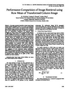
Figure 2. User interface of the system
vector of length 10. This wavelet-based feature has been proven to be quite effective in modeling image texture features [15,16]. The last visual feature we use is a recently developed water-fill edge feature [27]. The original image is first fed into the Canny edge detector to generate its corresponding edge map. The edge map is then considered as a network of tunnels. Virtual water is then poured into the tunnels. By measuring maximum filling time, maximum fork count, etc., this algorithm captures important edge characteristics of the original image. It extracts 18 elements in total [27]. One thing worth pointing out is that the adaptive filtering framework we proposed in this paper is an open framework. That is, the algorithm works regardless of which visual features are used. We use the above three visual features just for illustration purpose, more advanced feature (e.g., region layout, etc. [15]) can readily be incorporated into the system.
5.4. Performance measures The most widely used performance measures for information retrieval are precision (Pr) and recall (Re) [18]. Pr is defined as the number of retrieved relevant objects (i.e., N) over the number of total retrieved objects, say the top 20 images. Re is defined as the number of retrieved relevant objects over the total number of relevant objects in the image collection (in the Corel data set case, 99). The performance of an "ideal" system is to have both high Pr and Re. Unfortunately, Pr and Re are conflicting criteria and cannot be at high values at the same time. Because of this, instead of using a single value for Pr and Re, the Pr(Re) curve is normally used to characterize the performance of a retrieval system.
Table 1. Comparison between forward learning (LMS_F) and backward learning (LMS_B) for LMS. Precision (percentage) 0 iteration 1 iteration 2 iterations Return top LMS_F 14.48 16.83 17.50 20 LMS_B 14.41 18.96 20.41 Return top LMS_F 6.91 9.94 10.44 100 LMS_B 7.25 11.87 13.04 Return top LMS_F 6.18 7.15 9.08 180 LMS_B 5.73 9.09 9.58 Table 2. Comparison between forward learning (RLS_F) and backward learning (RLS_B) for RLS. Precision (percentage) 0 iteration 1 iteration 2 iterations Return top RLS_F 11.18 12.82 15.62 20 RLS_B 14.95 17.86 19.25 Return top RLS_F 7.04 9.68 11.83 100 RLS_B 7.23 10.41 11.07 Return top RLS_F 5.89 7.55 9.32 180 RLS_B 5.77 9.15 9.63
after two iterations of feedback. Similarly, Table 2 shows the forward/backward learning results for RLS, and Figure 4 shows their precision-recall curve. Regarding the forward learning and backward learning, following observations can be made based on the above tables and figures: •
Because the backward learning order simulates the “coarse-to-fine” learning process, it benefits the
5.5. System description We have developed a prototype system based on the proposed optimal adaptive filtering approaches. The system is written in C++ and running on Windows NT platform. Its interface is shown in Figure 2. Our prototype system has two modes: demo mode and testing mode. During the demo mode, a user can browse through the image collection and submit any image as the query image, which is shown at the top-left corner. For each of the returned image, there is a degree-of-relevance (i.e., similarity π(n)) slider to allow the user to provide his/her relevance feedback. During testing mode, the system uses the Corel high-level category information as the ground truth to obtain relevance feedback. This is a very challenging task and we next report detailed experimental results.
Figure 3. Comparison between forward learning and backward learning for LMS. Solid curve is for forward learning and dashed curve is for backward learning.
5.6. Results and observations 5.6.1. Forward learning vs. backward learning Table 1 shows the forward/backward learning results for LMS when the top 20, 100, and 180 most similar images are returned. To better compare the two learning orders, in Figure 3, we also plot the precision-recall curve for LMS
Figure 4. Comparison between forward learning and backward learning for RLS. Solid curve is for forward learning and dashed curve is for backward learning.
Table 3. Comparison between OPL, LMS with backward learning and RLS with backward learning. Precision (percentage) 0 iteration 1 iteration 2 iterations Return top OPL 10.18 14.18 15.85 20 LMS_B 14.41 18.96 20.41 RLS_B 14.95 17.86 19.25 Return top OPL 5.75 9.47 11.60 100 LMS_B 7.25 11.87 13.04 RLS_B 7.23 10.41 11.07 Return top OPL 4.63 7.78 9.39 180 LMS_B 5.73 9.09 9.58 RLS_B 5.77 9.15 9.63
adaptive filtering algorithms to fine-tune the weights at the last stage. For both LMS and RLS, the backward learning outperforms the forward learning. •
The ordering effect is more noticeable in LMS than in RLS. When the number of feedback examples is relatively large (e.g., the bottom-right portion of Figure 4), the forward and backward learning are almost the same for RLS. This is because RLS continuously learns all the examples, while LMS quickly adapts to the new example, forgetting the older ones.
5.6.2. LMS vs. RLS vs. OPL Table 3 shows the comparison between OPL, LMS with backward learning and RLS with backward learning when the top 20, 100, and 180 most similar images are returned, and Figure 5 shows their precision-recall curve after two iterations of relevance feedback. Based on the table and figure, the following observations can be made: • With more feedback iterations, the retrieval performance increases in all the three algorithms. • When the number of returned images is small (e.g., return top 20 images only), the performance of LMS and RLS is significantly better than that of OPL. This is because OPL switches to a diagonal matrix, resulting in sub-optimal solution (see Section 3). When the number of returned images is sufficiently large (e.g., 180 images), the performance of all the three algorithms is comparable. This is because, all the three algorithms are close to the optimal solution conditioned
Figure 5. Comparison between OPL, LMS, and RLS. The Solid curve represents OPL, dashed curve represents LMS and dotted curve represents RLS.
•
on the feedback examples. The LMS with backward learning seems to be the winning approach. Not only its retrieval performance is the best, its computation complexity is significantly cheaper than the other two approaches (see Section 4.5).
6. Conclusions Motivated by the fact that human’s vision system can be simulated by a signal filter, in this paper, we developed optimal adaptive filter based relevance feedback techniques for CBIR. Both LMS and RLS are effective in learning and efficient in computation. Furthermore, they both learn incrementally, i.e., they support on-line learning. This is particular useful in that when a new example arrives, the algorithms can learn without starting from scratch. Given the characteristics in CBIR, we further studied two learning orders (forward and backward) for the adaptive filters. The backward learning order is superior because it simulates a “coarse-to-fine” learning process. To evaluate the performance of the proposed approaches, we conducted extensive tests on a large-scale heterogeneous image collection and compared them against a state-of-the-art approach. Of equal importance, our study used high-level concepts, instead of low-level features, as the ground truth, which realistically meets average users’ image retrieval needs [14]. Experimental results show that LMS with backward learning is the winning technique that is both accurate and efficient.
7. Acknowledgement The Corel image set was obtained from Corel and used in accordance with their copyright statement. The first author is supported in part by China NSF grant 69902004.
Appendix A: RLS Algorithm for CBIR r For a finite time serial signal X (n) , we have r r n R xx (n) = ∑i =1 X (i) X (i ) T r n r P( n) = ∑i =1 X (i )d (i )
(A1)
Hence we have the following recursion for updating the covariance matrix and the cross-correlation vector r T r R xx (n) = R xx (n − 1) + X (n) X (n) r r r (A2) P(n) = P(n − 1) + X (n)d (n) A major obstacle we want to avoid is the matrix inversion of Rxx when solving for the optimal Wiener solution (see Equation (5)). The matrix inversion lemma helps us to overcome this difficulty. Let A, B, and F all be positive definite matrices, the matrix inversion lemma says [19], if (A3) A = B −1 + CF −1C T then (A4) A −1 = B − BC ( F + C T BC ) −1 C T B Because both R(n) and R(n-1) are positive definite, let r (A5) A = R ( n), B = R −1 ( n − 1), C = X (n), F = 1
For convenience, let’s further define Q(n) = R −1 (n), e(n) = d (n) − y(n)
(A6)
= − 2σ ln(π (n)) − W (n − 1) X (n) By substituting Equations (A5) and (A6) into (A4), we have r r (A7) Q(n) = Q(n − 1) − K (n) X T (n)Q(n − 1) where r 2
r K ( n) =
T
Q (n − 1) X (n) r r [1 + X T (n)Q (n − 1) X (n)]
(A8)
is called the gain vector. Rearranging the terms in Equation (A8), we have r r r r r K (n) = Q(n − 1) X (n) − K (n) X (n)T Q (n − 1) X (n) r r r (A9) = (Q(n − 1) − K (n) X (n)T Q(n − 1)) X (n) r = Q ( n) X ( n) To summarize, the recursive W(n) can be calculated as follows: r r W (n) = Rxx−1 (n) P (n) r = Q ( n) P ( n) r r = Q (n)[ P(n − 1) + X (n)d (n)] r r = Q (n −) P(n − 1) + Q (n) X ( n) d ( n) r r r r = Q ( n − 1) P (n − 1) − K (n) X ( n) T Q ( n − 1) P( n − 1) r + Q ( n) X ( n) d (n ) r r r r = W ( n − 1) + K (n)(d ( n) − X ( n) T W ( n − 1)) r r = W ( n − 1) + K (n)e( n)
References 1.
September 1999 Lee, H.K.; Yoo, S.I., A neural network-based image retrieval using nonlinear combination of heterogeneous features. Proc. of the 2000 Congress on Evolutionary Computation, Vol. 1, 2000, pp: 667 -674 10. Ma, W.; Zhang, H.J., Benchmarking of image features for content-based retrieval. Proc. Of the Thirty-Second Asilomar Conference on Signals, Systems & Computers, Vol. 1, 1998, pp: 253 –257. 11. MacArthur, S.D.; Brodley, C.E.; Shyu, C., Relevance feedback decision trees in content-based image retrieval, Proc. IEEE Workshop on Content-based Access of Image and Video Libraries, 2000, pp: 68 –72.
9.
Bergen, J. and Adelson, E.H. Hierarchical, Computationally Efficient Motion Estimation Algorithm. J. of the Optical Society of America A, 4:35, 1987 2. Communication of the ACM, Special issue on “Digital Library”, Guest editors: Edward Fox and Gary Marchionini, May 2001, Vol. 44, No. 5. 3. Cox, I.J.; Miller, M.L.; Minka, T.P.; Papathomas, T.V.; Yianilos, P.N., The Bayesian image retrieval system, Pichunter: theory, implementation, and psychophysical experiments. IEEE Trans. on Image Processing, Vol. 9(3), March 2000, pp: 524 –524. 4. Cox, I.J., Miller, M.L, Omohundro, S.M., and Yianilos, P.N., PicHunter: Bayesian Relevance Feedback for Image Retrieval," Proc. Int. Conf. on Pattern Recognition, Vienna, Austria, C:361-369, August 1996 5. Daubechies, I., Ten Lectures on Wavelets, CBMS-NSF Lecture Notes nr. 61, SIAM, 1992. 6. IEEE Computer Magazine, Special Issue on “Content-based image retrieval systems”, Guest editors: Venkat N. Gudivada and Jijay V. Raghavan, 1995, Vol. 28, No. 9. 7. Ishikawa, Y.; Subramanya, R. and Faloutsos, C., Mindreader: Query databases through multiple examples. Proc. of the 24th VLDB Conference (New York), 1998. 8. Lee, C., Ma, W. Y., and Zhang, H.J., Information embedding based on user’s relevance feedback for image retrieval, Proc. of Multimedia Storage and Archiving Systems IV, Boston,
12. Minka, T., and Picard, R., Interactive learning using a society of models, Pattern Recognition, Special issue on Image Databases, 30(4), 1997 13. Peng, J., Adaptive multi-class metric content-based image retrieval, Proc. of the 4th Int. Conference on Visual Information Systems , Lyon, France, November 2-4. 14. Rodden, K., Basalaj, W., Sinclair, D., and Wood, K., Does organization by similarity assist image browsing, Proc. ACM Compute-Human Interaction (CHI), 2000. pp. 190-197. 15. Rui, Y.; Huang, T. and Chang, S. F., Image retrieval: current techniques, promising directions and open issues, Journal of Visual Communication and Image Representation , Vol. 10, 39-62, March, 1999 16. Rui, Y.; Huang, T. and Mehrotra, S., Content-based image retrieval with relevance feedback in MARS. Proc. IEEE Int. Conf. on Image Processing, 1997 17. Rui, Y.; Huang, T. Optimizing learning in image retrieval. Proc. IEEE Int. Conf. on Computer Vision and Pattern Recognition, Vol. 1, 2000, pp: 236 –243. 18. Salton, G., and McGill, M. J., Introduction to modern information retrieval, McGraw-Hill Book Company, New York, 1982. 19. Simon Haykin, Adaptive filter theory, 3rd ed., Upper Saddle River, N.J: Prentice Hall, 1996, Prentice Hall information and system sciences series. 20. Smeulders, A. W. M.; Worring, M.; Santini, S.; et al. Content-based image retrieval at the end of the early years, IEEE Trans. PAMI, Vol. 22(12), Dec. 2000 pp: 1349 –1380. 21. Swets, D.L.; Weng, J.J. Using discriminant eigen-features for image retrieval, IEEE Trans PAMI, Vol. 18(8), Aug. 1996, pp: 831 –836 22. Tian Q. Hong, P., Huang, T. S., Update relevant image weights for content-based image retrieval using support vector machines, Proc. IEEE Int. Conf. On Multimedia and Expo, Vol. 2, pp: 1199-1202, 2000. 23. Tieu, K.; Viola, P. Boosting image retrieval. Proc. IEEE CVPR, Vol. 1, 2000, pp: 228 –235. 24. Vasconcelos, N.; Lippman, A. A probabilistic architecture for content-based image retrieval, Proc. IEEE CVPR, Vol. 1, 2000 pp: 216 –221. 25. Widrow, B., and Hoff, M. E., Adaptive switching circuits, IRE WESCON Conv. Rec., pp. 96-104. 26. Wu, Y.; Tian, Q.; Huang, T.S., Discriminant-EM algorithm with application to image retrieval. Proc. IEEE CVPR, Vol. 1, 2000, pp: 222 –227. 27. Zhou, X., Rui, Y., and Huang, T.S., Water-Filling Algorithm: A Novel Way for Image Feature Extraction based on Edge Maps, Proc. of IEEE ICIP 1999, Kobe, Japan.