Optimal and Suboptimal Singleton Arc Consistency Algorithms Christian Bessiere LIRMM (CNRS / University of Montpellier) 161 rue Ada, Montpellier, France
[email protected]
Abstract Singleton arc consistency (SAC) enhances the pruning capability of arc consistency by ensuring that the network cannot become arc inconsistent after the assignment of a value to a variable. Algorithms have already been proposed to enforce SAC, but they are far from optimal time complexity. We give a lower bound to the time complexity of enforcing SAC, and we propose an algorithm that achieves this complexity, thus being optimal. However, it can be costly in space on large problems. We then propose another SAC algorithm that trades time optimality for a better space complexity. Nevertheless, this last algorithm has a better worst-case time complexity than previously published SAC algorithms. An experimental study shows the good performance of the new algorithms.
1 Introduction Ensuring that a given local consistency does not lead to a failure when we enforce it after having assigned a variable to a value is a common idea in constraint reasoning. It has been applied (sometimes under the name ’shaving’) in constraint problems with numerical domains by limiting the assignments to bounds in the domains and ensuring that bounds consistency does not fail [Lhomme, 1993]. In SAT, it has been used as a way to compute more accurate heuristics for DPLL [Freeman, 1995; Li and Ambulagan, 1997]. Finally, in constraint satisfaction problems (CSPs), it has been introduced under the name Singleton Arc Consistency (SAC) in [Debruyne and Bessi`ere, 1997b] and further studied, both theoretically and experimentally in [Prosser et al., 2000; Debruyne and Bessi`ere, 2001]. Some nice properties give to SAC a real advantage over the other local consistencies enhancing the ubiquitous arc consistency. Its definition is much simpler than restricted path consistency [Berlandier, 1995], max-restricted-path consistency [Debruyne and Bessi`ere, 1997a], or other exotic local consistencies. Its operational semantics can be understood by a non-expert of the field. Enforcing it only removes values in domains, and thus does not change the structure of the problem, as opposed to path consistency [Montanari, 1974], k-
Romuald Debruyne ´ Ecole des Mines de Nantes / LINA 4 rue Alfred Kastler, Nantes, France
[email protected]
consistency [Freuder, 1978], etc. Finally, implementing it can be done simply on top of any AC algorithm. Algorithms enforcing SAC were already proposed in the past (SAC1 [Debruyne and Bessi`ere, 1997b], and SAC2 [Bart´ak and Erben, 2004]) but they are far from optimal time complexity. Moreover, singleton arc consistency lacks an analysis of its complexity. In this paper, we study the complexity of enforcing SAC (in Section 3) and propose an algorithm, SAC-Opt, enforcing SAC with optimal worst-case time complexity (Section 4). However, optimal time complexity is reached at the cost of a high space complexity that prevents the use of this algorithm on large problems. In Section 5, we propose SAC-SDS, a SAC algorithm with better worst-case space complexity but no longer optimal in time. Nevertheless, its time complexity remains better than the SAC algorithms proposed in the past. The experiments presented in Section 6 show the good performance of both SAC-Opt and SAC-SDS compared to previous SAC algorithms.
2 Preliminaries A constraint network P consists of a finite set of n variables X = {i, j, . . .}, a set of domains D = {D(i), D(j), . . .}, where the domain D(i) is the finite set of at most d values that variable i can take, and a set of e constraints C = {c1 , . . . , ce }. Each constraint ck is defined by the ordered set var(ck ) of the variables it involves, and the set sol(ck ) of combinations of values satisfying it. A solution to a constraint network is an assignment of a value from its domain to each variable such that every constraint in the network is satisfied. When var(c) = (i, j), we use cij to denote sol(c) and we say that c is binary. A value a in the domain of a variable i (denoted by (i, a)) is consistent with a constraint ck iff there exists a support for (i, a) on ck , i.e., an instantiation of the other variables in var(ck ) to values in their domain such that together with (i, a) they satisfy ck . Otherwise, (i, a) is said arc inconsistent. A constraint network P = (X, D, C) is arc consistent iff D does not contain any arc inconsistent value. AC(P ) denotes the network where all arc inconsistent values have been removed from P . If AC(P ) has empty domain, we say that P is arc inconsistent Definition 1 (Singleton arc consistency) A constraint network P = (X, D, C) is singleton arc consistent iff ∀i ∈
X, ∀a ∈ D(i), the network P |i=a = (X, D|i=a , C) obtained by replacing D(i) by the singleton {a} is not arc inconsistent. If P |i=a is arc inconsistent, we say that (i, a) is SAC inconsistent.
3 Complexity of SAC Both SAC1 [Debruyne and Bessi`ere, 1997b] and SAC2 [Bart´ak and Erben, 2004] have an O(en2 d4 ) time complexity on binary constraints. But it is not optimal. Theorem 1 The best time complexity we can expect from an algorithm enforcing SAC on binary constraints is in O(end3 ). Proof. According to [McGregor, 1979], we know that checking whether a value (i, a) is such that AC does not fail in P |i=a is equivalent to verifying if in each domain D(j) there is at least one value b such that ((i, a), (j, b)) is “path consistent on (i, a)”. (A pair of values ((i, a)(j, b)) is path consistent on (i, a) iff it is not deleted when enforcing path consistency only on pairs involving (i, a).) For each variable j, we have to find a value b ∈ D(j) such that ((i, a), (j, b)) is path consistent on (i, a). In the worst case, all the values b in D(j) have to be considered. So, the path consistency of each pair ((i, a), (j, b)) may need to be checked against every third variable k by looking for a value (k, c) compatible with both (i, a) and (j, b). However, it is useless to consider variables k not linked to j since in this partial form of path consistency only pairs involving (i, a) can be removed. By using an optimal time path consistency technique (storing supports), we are guaranteed to consider at most once each value (k, c) when seeking compatible value on k for a pair ((i, a), (j, b)). The worst-case complexity of proving that path consistency on (i, a) does not fail is thus Σb∈D(j) Σckj ∈C Σc∈D(k) = ed2 . Furthermore, enforcing path consistency on (i, a) is completely independent from enforcing path consistency on another value (j, b). Indeed, a pair ((i, a), (j, b)) can be path consistent on (i, a) while becoming path inconsistent after the deletion of a pair ((k, c), (j, b)) thus being path inconsistent on (j, b). Therefore, the worst case time complexity of any SAC algorithm is at least in O(Σ(i,a)∈D ed2 ) = O(end3 ). 2
4 Optimal Time Algorithm for SAC SAC1 has no data structure storing which values may become SAC inconsistent when a given value is removed. Hence, it must check again the SAC consistency of all remaining values. SAC2 has data structures that use the fact that if AC does not lead to a wipe out in P |i=a then the SAC consistency of (i, a) holds as long as all the values in AC(P |i=a ) are in the domain. After the removal of a value (j, b), SAC2 checks again the SAC consistency of all the values (i, a) such that (j, b) was in AC(P |i=a ). This leads to a better average time complexity than SAC1 but the data structures of SAC2 are not sufficient to reach optimality since SAC2 may waste time re-enforcing AC in P |i=a several times from scratch. Algorithm 1, called SAC-Opt, is an algorithm that enforces SAC in O(end3 ), the lowest time complexity which can be expected (see Theorem 1). The idea behind such an optimal algorithm is that we don’t want to do and redo (potentially nd times) arc consistency
Algorithm 1: The optimal SAC algorithm function SAC-Opt(inout P : Problem): Boolean; /* init phase */; 1 if AC(P ) then PendingList ← ∅ else return false; 2 foreach (i, a) ∈ D do 3 Pia ← P /* copy only domains and data structures */; 4 Dia (i) ← {a}; 5 if ¬propagAC(Pia , D(i) \ {a}) then 6 D ← D \ {(i, a)}; 7 if propagAC(P, {(i, a)}) then 8 foreach Pjb such that (i, a) ∈ Djb do 9 Qjb ← Qjb ∪ {(i, a)}; 10 PendingList ← PendingList ∪ {(j, b)}; 11 else return false; 12 13 14 15 16 17 18 19 20 21
/* propag phase */; while PendingList 6= ∅ do pop (i, a) from PendingList; if propagAC(Pia , Qia ) then Qia ← ∅; else D ← D \ {(i, a)}; if D(i) = ∅ then return false; foreach (j, b) ∈ D such that (i, a) ∈ Djb do Djb (i) ← Djb (i) \ {a}; Qjb ← Qjb ∪ {(i, a)}; PendingList ← PendingList ∪ {(j, b)}; return true;
from scratch in each subproblem P |j=b each time a value (i, a) is found SAC inconsistent. (Which represents n2 d2 potential arc consistency calls.) To avoid such costly repetitions of arc consistency calls, we duplicate the problem nd times, one for each value (i, a), so that we can benefit from the incrementality of arc consistency on each of them. All generic AC algorithms are incremental, i.e., their complexity on a problem P is the same for a single call or for up to nd calls, where two consecutive calls differ only by the deletion of some values from P . In the following, Pia is the subproblem in which SACOpt stores the current domain (noted Dia ) and the data structure corresponding to the AC enforcement in P |i=a . propagAC(P, Q) denotes the function that incrementally propagates the removal of set Q of values in problem P when an initial AC call has already been executed, initialising the data structure required by the AC algorithm in use. It returns false iff P is arc inconsistent. SAC-Opt is composed of two main steps. After making the problem arc consistent (line 1), the loop in line 2 takes each value a in each domain D(i) and creates the problem Pia as a copy of the current P . Then, in line 5 the removal of all the values different from a for i is propagated. If a subproblem Pia is arc inconsistent, (i, a) is pruned from the ’master’ problem P and its removal is propagated in P (line 7). The advantage of propagating immediately in the master problem the SAC inconsistent values found in line 5 is twofold. First, the subproblem Pkc of a value (k, c) removed in line 7 before its selection in line 2 will never be created. Second, the subproblems Pjb created after the removal of (k, c) will benefit from this propagation since they are created by duplication of P (line 3). For each already created subproblem Pjb with a ∈ Djb (i), (i, a) is put in Qjb and Pjb is put in PendingList
for future propagation (lines 9–10). Once the initialisation phase has finished, we know that PendingList contains all values (i, a) for which some SAC inconsistent value removals (contained in Qia ) have not yet been propagated in Pia . The loop in line 12 propagates these removals (line 14). When propagation fails, this means that (i, a) itself is SAC inconsistent. It is removed from the domain D of the master problem in line 16 and each subproblem Pjb containing (i, a) is updated together with its propagation list Qjb for future propagation (lines 18–20). When PendingList is empty, all removals have been propagated in the subproblems. So, all the values in D are SAC. Theorem 2 SAC-Opt is a correct SAC algorithm with O(end3 ) optimal time complexity and O(end2 ) space complexity on binary constraints. Proof. Soundness. A value a is removed from D(i) either in line 6 or in line 16 because Pia was found arc inconsistent. If Pia was found arc inconsistent in the initialisation phase (line 5), SAC inconsistency of (i, a) follows immediately. Let us proceed by induction for the remaining case. Suppose all values already removed in line 16 were SAC inconsistent. If Pia is found arc inconsistent in line 14, this means that Pia cannot be made arc consistent without containing some SAC inconsistent values. So, (i, a) is SAC inconsistent and SACOpt is sound. Completeness. Thanks to the way PendingList and Qia are updated in lines 8–10 and 18–20, we know that at the end of the algorithm, all Pia are arc consistent. Thus, for any value (i, a) remaining in P at the end of SAC-Opt, P |i=a is not arc inconsistent and (i, a) is therefore SAC consistent. Complexity. The complexity analysis is given for networks of binary constraints since the optimality proof was given for networks of binary constraints only. (But SAC-Opt works on constraints of any arity.) Since any AC algorithm can be used to implement our SAC algorithm, the space and time complexities will obviously depend on this choice. Let us first discuss the case where an optimal time algorithm such as AC-6 [Bessi`ere, 1994] or AC2001 [Bessi`ere and R´egin, 2001; Zhang and Yap, 2001] is used. Line 3 tells us that the space complexity will be nd times the complexity of the AC algorithm, namely O(end2 ). Regarding time complexity, the first loop copies the data structures and propagates arc consistency on each subproblem (line 5), two tasks which are respectively in nd · ed and nd · ed2 . In the while loop (line 12), each subproblem can be called nd times for arc consistency, and there are nd subproblems. Now, AC-6 and AC2001 are both incremental, which means that the complexity of nd restrictions on the same problem is ed2 and not nd · ed2 . Thus the total cost of arc consistency propagation on the nd subproblems is nd · ed2 . We have to add the cost of updating the lists in lines 8 and 18. In the worst case, each value is removed one by one, and thus, nd values are put in nd Q lists, leading to n2 d2 updates of PendingList. If n < e, the total time complexity is O(end3 ), which is optimal. 2 Remarks. We chose to present the Qia lists as lists of values to be propagated because the AC algorithm used is not specified here, and value removal is the most accurate information we can have. When using a fine-grained AC algorithm,
such as AC-6 the lists will be used as they are. If we use a coarse-grained algorithm such as AC-3 [Mackworth, 1977] or AC2001, only the variables from which the domain has changed are needed. The modification is direct. We should bear in mind that if AC-3 is used, we decrease space complexity to O(n2 d2 ), but time complexity increases to O(end4 ) since AC-3 is non optimal.
5 Losing Time Optimality to Save Space SAC-Opt cannot be used on large constraint networks because of its O(end2 ) space complexity. Moreover, it seems difficult to reach optimal time complexity with smaller space requirements. A SAC algorithm has to maintain AC on nd subproblems P |i=a , and to guarantee O(ed2 ) total time on these subproblems we need to use an optimal time AC algorithm. Since there does not exist any optimal AC algorithm requiring less than O(ed) space, we obtain nd · ed space for the whole SAC process. We propose to relax time optimality to reach a satisfactory trade-off between space and time. To avoid discussing in too general terms, we instantiate this idea on a AC2001-based SAC algorithm for binary constraints, but the same idea could be implemented with other optimal AC algorithms such as AC-6, and with constraints of any arity. The algorithm SACSDS (Sharing Data Structures) tries to use as much as possible the incrementality of AC to avoid redundant work, without duplicating on each subproblem P |i=a the data structures required by optimal AC algorithms. This algorithm requires less space than SAC-Opt but is not optimal in time. As in SAC-Opt, for each value (i, a) SAC-SDS stores the local domain Dia of the subproblem P |i=a and its propagation list Qia . Note that in our AC2001-like presentation, Qia is a list of variables j for which the domain Dia (j) has changed (in SAC-Opt it is a list of values (j, b) removed from Dia ). As in SAC-Opt, thanks to these local domains Dia , we know which values (i, a) may no longer be SAC after the removal of a value (j, b): those for which (j, b) was in Dia . These local domains are also used to avoid starting each new AC propagation phase from scratch, since Dia is exactly the domain from which we should start when enforcing again AC on P |i=a after a value removal. By comparison, SAC1 and SAC2 restart from scratch for each new propagation. But the main idea in SAC-SDS is that as opposed to SACOpt, it does not duplicate to all subproblems Pia the data structures of the optimal AC algorithm used. The data structure is maintained only in the master problem P . In the case of AC2001, the Last structure which maintains in Last(i, a, j) the smallest value in D(j) compatible with (i, a) on cij is built and updated only in P . Nevertheless, it is used by all subproblems Pia to avoid repeating constraint checks already done in P . SAC-SDS (Algorithm 2) works as follows: After some initialisations (lines 1–4), SAC-SDS repeatedly pops a value from PendingList and propagates AC in Pia (lines 6–9). Note that ’Dia =nil’ means that this is the first enforcement of AC in Pia , so Dia must be initialised (line 8).1 If Pia is arc in1 We included this initialisation step in the main loop to avoid repeating similar lines of code, but a better implementation will put
Algorithm 2: The SAC-SDS algorithm function SAC-SDS-2001(inout P : problem): Boolean; if AC2001(P ) then PendingList ← ∅ else return false; foreach (i, a) ∈ D do Dia ← nil ; Qia ← {i}; PendingList ← PendingList ∪ {(i, a)}; 5 while PendingList 6= ∅ do 6 pop (i, a) from PendingList ; 7 if a ∈ D(i) then 8 if Dia = nil then Dia ← (D \ D(i)) ∪ {(i, a)}; 9 if propagSubAC(Dia , Qia ) then Qia ← ∅; 10 else 11 D(i) ← D(i) \ {a} ; Deleted ← {(i, a)} ; 12 if propagMainAC(D, {i}, Deleted) then 13 updateSubProblems(Deleted) 14 else return false; 15 return true; 1 2 3 4
function Propag Main/Sub AC(inout D: domain; in Q: set ; 16 17 18 19 20 21 22 23 24 25 26
inout Deleted: set ): Boolean; while Q 6= ∅ do pop j from Q ; foreach i ∈ X such that ∃cij ∈ C do foreach a ∈ D(i) such that Last(i, a, j) 6∈ D(j) do if ∃b ∈ D(j), b > Last(i, a, j) ∧ cij (a, b) then Last(i, a, j) ← b else D(i) ← D(i) \ {a} ; Q ← Q ∪ {i} ; Deleted ← Deleted ∪ {(i, a)} ; if D(i) = ∅ then return false; return true; /* · · · : in propagMainAC but not in propagSubAC */;
procedure updateSubProblems(in Deleted: set); foreach (j, b) ∈ D | Djb ∩ Deleted 6= ∅ do Qjb ← Qjb ∪ {i ∈ X / Djb (i) ∩ Deleted 6= ∅} ; Djb ← Djb \ Deleted; PendingList ← PendingList ∪ {(j, b)} ;
27 28 29 30
consistent, (i, a) is SAC inconsistent. It is therefore removed from D (line 11) and this deletion is propagated in the master problem P using propagMainAC (line 12). Any value (i, a) removed from P is put in the set Deleted (lines 11 and 24). This set is used by updateSubProblems (line 13) to pass the values removed from P on to the subproblems, and to update the lists Qjb and PendingList for further propagation in modified subproblems. At this point we have to explain the difference between propagMainAC, which propagates deletions in the master problem P , and propagSubAC, which propagates deletions in subproblems Pia . The parts that are in boxes belong to propagMainAC and not to propagSubAC. Function propagSubAC, used to propagate arc consistency in the subproblems, follows the same principle as the AC algorithm. The only difference comes from the fact that the data structures of the AC algorithm are not modified. When using AC2001, this means that Last is not updated in line 21. Indeed, this data structure is useful to achieve AC in the subit in a former loop as in SAC-Opt.
problems faster (lines 19–20) since we know that there is no support for (i, a) on cij lower than Last(i, a, j) in P , and so in any subproblem as well. But this data structure is shared by all subproblems. Thus it must not be modified by propagSubAC. Otherwise, Last(i, a, j) would not be guaranteed to be the smallest support in the other subproblems and in P . When achieving AC in P , propagMainAC does update the Last data structure. The only difference with AC2001 is line 24 where it needs to store in Deleted the values removed from D during the propagation. Those removals performed in P can directly be transferred in the subproblems without the effort of proving their inconsistency in each subproblem. This is done via function updateSubProblems, which removes values in Deleted from all the subproblems. It also updates the local propagation lists Qia and PendingList for future propagation in the subproblems. Theorem 3 SAC-SDS is a correct SAC algorithm with O(end4 ) time complexity and O(n2 d2 ) space complexity on binary constraints. Proof. Soundness. Note first that the structure Last is updated only when achieving AC in P so that any support of (i, a) in D(j) is greater than or equal to Last(i, a, j). The domains of the subproblems being subdomains of D, any support of a value (i, a) on cij in a subproblem is also greater than or equal to Last(i, a, j). This explains that propagSubAC can benefit from the structure Last without losing any support (lines 19–20). Once this observation is made, soundness comes from the same reason as in SAC-Opt. Completeness. Completeness comes from the fact that any deletion is propagated. After initialisation (lines 2-4), PendingList = D and so, the main loop of SAC-SDS processes any subproblem P |i=a at least once. Each time a value (i, a) is found SAC inconsistent in P because P |i=a is arc inconsistent (line 9) or because the deletion of some SAC-inconsistent value makes it arc inconsistent in P (line 23 of propagMainAC called in line 12), (i, a) is removed from the subproblems (line 29), and PendingList and the local propagation lists are updated for future propagation (lines 28 and 30). At the end of the main loop, PendingList is empty, so all the removals have been propagated and for any value (i, a) ∈ D, Dia is a non empty arc consistent subdomain of P |i=a . Complexity. The data structure Last requires a space in O(ed). Each of the nd domains Dia can contain nd values and there is at most n variables in the nd local propagation lists Qia . Since e < n2 , the space complexity of SAC-SDS2001 is in O(n2 d2 ). So, considering space requirements, SAC-SDS-2001 is similar to SAC2. Regarding time complexity, SAC-SDS-2001 first duplicates the domains and propagates arc consistency on each subproblem (lines 8 and 9), two tasks which are respectively in nd·nd and nd · ed2 . Each value removal is propagated to all P |i=a problems via an update of PendingList, Qia and Dia (lines 27–30). This requires nd · nd operations. Each subproblem can in the worst case be called nd times for arc consistency, and there are nd subproblems. The domains of each subproblem are stored so that the AC propagation is launched with the domains in the state in which they were at the end of the
1E+4
cpu time (in sec.) n=100, d=20, and density=.05
1500
cpu time (in sec.) n=100, d=20, and density=1 (complete constraint networks)
1E+1
1400 1300 1200 1100
1E+3
1000
Zoom with a non logarithmic scale
900 800
700 1E0
600
1E+2
500 400 16
300
14
200 1E+1
100
12
0 .38
10
1E-1
.39
.40
.41
.42
.43
.44
.45
8 6 SAC-Opt-2001
SAC-SDS-2001
SAC-1-2001
SAC-2-2001
SAC-1-6
SAC-2-6
SAC-1-4
SAC-2-4
0 .67
.15
.20
.25
.30
.35
.40
.45
.50
.69
.71
.55
.73
.60
.75
Tightness
.77
.65
SAC-SDS-2001
SAC-Opt-2001
2
1E-2 .10
1E0
Zoom with a non logarithmic scale
4
SAC-1-2001
SAC-2-2001
SAC-1-6
SAC-2-6
Tightness
SAC-2-4
SAC-1-4 1E-1
.70
.75
.80
.85
.90
Figure 1: cpu time with n = 100, d = 20, and density= .05. previous AC propagation in the subproblem. Thus, in spite of the several AC propagations on a subproblem, a value will be removed at most once and, thanks to incrementality of arc consistency, the propagation of these nd value removals is in O(ed3 ). (Note that we cannot reach the optimal ed2 complexity for arc consistency on these subproblems since we do not duplicate the data structures necessary for AC optimality.) Therefore, the total cost of arc consistency propagations is nd · ed3 . The total time complexity is O(end4 ). 2 As with SAC2, SAC-SDS performs a better propagation than SAC1 since after the removal of a value (i, a) from D, SAC-SDS checks the arc consistency of the subproblems P |j=b only if they have (i, a) in their domains (and not all the subproblems as SAC1). But this is not sufficient to have a better worst-case time complexity than SAC1. SAC2 has indeed the same O(en2 d4 ) time complexity as SAC1. SAC-SDS improves this complexity because it stores the current domain of each subproblem, and so, does not propagate in the subproblems each time from scratch.2 Furthermore, we can expect a better average time complexity since the shared structure Last reduces the number of constraint checks required, even if it does not permit to obtain optimal worst-case time complexity. This potential gain can only be assessed by an experimental comparison of the different SAC versions. Finally, in SAC1 and SAC2 each AC enforcement in a subproblem must be done on a new copy of D built at runtime (potentially nd · nd times) while such duplication is performed only once for each value in SAC-SDS (by creating subdomains Dia ).
6 Experimental Results We compared the performance of the SAC algorithms on random uniform constraint networks of binary constraints generated by [Frost et al., 1996], which produces instances accord2 This is independent on the AC algorithm used and so, enforcing AC with AC-3 preserves this O(end4 ) time complexity.
.10
.15
.20
.25
.30
.35
.40
.45
.50
.55
.60
.65
.70
.75
.80
.85
.90
Figure 2: cpu time with n = 100, d = 20, and density= 1.
ing to Model B [Prosser, 1996]. All algorithms have been implemented in C++ and ran on a Pentium IV-1600 MHz with 512 Mb of memory under Windows XP. SAC1 and SAC2 have been tested using several AC algorithms. In the following, we note SAC-1-X, SAC-2-X and SAC-Opt-X the versions of SAC1, SAC2 and SAC-Opt based on AC-X. Note that for SAC2 the implementation of the propagation list has been done according to the recommendations made in [Bart´ak and Erben, 2003]. For each combination of parameters tested, we generated 50 instances for which we report mean cpu times.
6.1
Experiments on sparse constraint networks
Fig. 1 presents performance on constraint networks having 100 variables, 20 values in each domain, and a density of .05. These constraint networks are relatively sparse since the variables have five neighbours on average. For a tightness lower than .55, all the values are SAC. On these under-constrained networks, the SAC algorithms check the arc consistency of each subproblem at most once. Storing support lists (as in SAC2) or local subdomains (as in SACOpt and SAC-SDS) does not pay-off. A brute-force algorithm such as SAC1 is sufficient. SAC-1-2001 shows the best performance. On problems having tighter constraints, some SAC inconsistent values are removed and at tightness .72 we can see a peak of complexity. However, as mentioned in [Bart´ak and Erben, 2003], the improved propagation of SAC2 is useless on sparse constraint networks and SAC2-X (with X∈ {4, 6, 2001}) is always more expensive than SAC1-X on the generated problems. Around the peak of complexity, SACSDS-2001 is the clear winner. SAC-Opt-2001 and SAC1-2001 are around 1.7 times slower, and all the others are between 2.1 and 10 times slower.
6.2
Experiments on dense constraint networks
Fig. 2 presents performance on constraint networks having 100 variables, 20 values in each domain and a complete graph of binary constraints. SAC1 and SAC2 show very close performance. When all values are SAC consistent (tightness lower than .37) the additional data structure of SAC2 is useless since there is no propagation. However the cost of building this data structure is not important compared to the overall time and the time required by SAC2 is almost the same as SAC1. Around the peak of complexity, SAC2-X (with X∈ {4, 6, 2001}) requires a little less time than SAC1-X. SAC2 has to repeatedly recheck the arc consistency of less subproblems than SAC1 but the cost of testing a subproblem remains the same. On very tight constraints, SAC1 requires less time than SAC2 since the inconsistency of the problem is found with almost no propagation and building the data structure of SAC2 is useless. Conversely to what was expected in [Bart´ak and Erben, 2004], using AC-4 in SAC1 (or in SAC2) instead of AC-6 or AC2001 is not worthwhile. The intuition was that since the data structure of AC-4 does not have to be updated, the cost of its creation would be low compared to the profit we can expect. However, SAC1-4 and SAC2-4 are far more costly than the versions based on AC-6 or AC2001. The best results are obtained with SAC-Opt-2001 and SACSDS-2001 which are between 2.6 and 17 times faster than the others at the peak. These two algorithms have a better propagation between subproblems than SAC1 but they also avoid some redundant work and so reduce the work performed on each subproblem.
7 Summary and Conclusion We have presented SAC-Opt, the first optimal time SAC algorithm. However, the high space complexity of this algorithm prevents its use on large constraint networks. Hence, we have proposed SAC-SDS, a SAC algorithm that is not optimal in time but that requires less space than SAC-Opt. Experiments show the good performance of these new SAC algorithms compared to previous versions available in the literature. This opens again the issue of using SAC as an alternative to AC for pruning values in a constraint network, or at least in ’promising’ parts of the network. SAC could also be used to compute variable selection heuristics, as this had been done with success in SAT [Li and Ambulagan, 1997].
References [Bart´ak and Erben, 2003] R. Bart´ak and R. Erben. Singleton arc consistency revised. In ITI Series 2003-153, Prague, 2003. [Bart´ak and Erben, 2004] R. Bart´ak and R. Erben. A new algorithm for singleton arc consistency. In Proceedings FLAIRS’04, Miami Beach FL, 2004. AAAI Press. [Berlandier, 1995] P. Berlandier. Improving domain filtering using restricted path consistency. In Proceedings IEEECAIA’95, 1995.
[Bessi`ere and R´egin, 2001] C. Bessi`ere and J.C. R´egin. Refining the basic constraint propagation algorithm. In Proceedings IJCAI’01, pages 309–315, Seattle WA, 2001. [Bessi`ere, 1994] C. Bessi`ere. Arc-consistency and arcconsistency again. Artificial Intelligence, 65:179–190, 1994. [Debruyne and Bessi`ere, 1997a] R. Debruyne and C. Bessi`ere. From restricted path consistency to max-restricted path consistency. In Proceedings CP’97, pages 312–326, Linz, Austria, 1997. [Debruyne and Bessi`ere, 1997b] R. Debruyne and C. Bessi`ere. Some practicable filtering techniques for the constraint satisfaction problem. In Proceedings IJCAI’97, pages 412–417, Nagoya, Japan, 1997. [Debruyne and Bessi`ere, 2001] R. Debruyne and C. Bessi`ere. Domain filtering consistencies. Journal of Artificial Intelligence Research, 14:205–230, 2001. [Freeman, 1995] J.W. Freeman. Improvements to propositional satisfiability search algorithms. PhD thesis, University of Pennsylvania, Philadelphia PA, 1995. [Freuder, 1978] E.C. Freuder. Synthesizing constraint expressions. Communications of the ACM, 21(11):958–966, Nov 1978. [Frost et al., 1996] D. Frost, C. Bessi`ere, R. Dechter, and J.C. R´egin. Random uniform csp generators. URL: http://www.lirmm.fr/˜bessiere/generator.html, 1996. [Lhomme, 1993] O. Lhomme. Consistency techniques for numeric csps. In Proceedings IJCAI’93, pages 232–238, Chamb´ery, France, 1993. [Li and Ambulagan, 1997] C.M. Li and Ambulagan. Heuristics based on unit propagation for satisfiability problems. In Proceedings IJCAI’97, pages 366–371, Nagoya, Japan, 1997. [Mackworth, 1977] A.K. Mackworth. Consistency in networks of relations. Artificial Intelligence, 8:99–118, 1977. [McGregor, 1979] J.J. McGregor. Relational consistency algorithms and their application in finding subgraph and graph isomorphism. Information Science, 19:229–250, 1979. [Montanari, 1974] U. Montanari. Networks of constraints: Fundamental properties and applications to picture processing. Information Science, 7:95–132, 1974. [Prosser et al., 2000] P. Prosser, K. Stergiou, and T Walsh. Singleton consistencies. In Proceedings CP’00, pages 353–368, Singapore, 2000. [Prosser, 1996] P. Prosser. An empirical study of phase transition in binary constraint satisfaction problems. Artificial Intelligence, 81:81–109, 1996. [Zhang and Yap, 2001] Y. Zhang and R.H.C. Yap. Making AC-3 an optimal algorithm. In Proceedings IJCAI’01, pages 316–321, Seattle WA, 2001.