WCCI 2012 IEEE World Congress on Computational Intelligence June, 10-15, 2012 - Brisbane, Australia
IJCNN
Optimal control design for nonlinear systems: Adaptive dynamic programming based on fuzzy critic estimator Jilie Zhang∗ , Huaguang Zhang† , Yanhong Luo‡ and Hongjing Liang
§
∗
School of Information Science and Engineering, Northeastern University, Shenyang, Liaoning 110819, P. R. China Email:
[email protected] † School of Information Science and Engineering, Northeastern University, and State Key Laboratory of Synthetical Automation for Process Industries (Northeastern University), Shenyang, Liaoning,110819, China. Email:
[email protected] ‡ School of Information Science and Engineering, Northeastern University, Shenyang, Liaoning 110819, P. R. China Email:
[email protected] § School of Information Science and Engineering, Northeastern University, Shenyang, Liaoning 110819, P. R. China Email:
[email protected]
Abstract—In this paper, an optimal control design approach based on fuzzy critic estimator (FCE) is presented for nonlinear continuous-time systems. The main idea of our study is to approximate the solution (i.e., value function) of the HamiltonJacobi-Bellman (HJB) equation by making use of FCE as an estimator/approximator, which is utilized to obtain the optimal control. The value function is estimated by FHM, which captures the mapping between the state and value function. Firstly, we illustrate the design process of the optimal control involving nonlinear systems. Secondly, we analyze the stability conditions and prove the approximate error is uniformly ultimately bounded (UUB). Finally, a numerical example is given to illustrate the effectiveness and advantages of our approach.
I. I NTRODUCTION In recent years, the adaptive dynamic programming (ADP) control of continuous-time systems was concerned by some researchers. Meanwhile , some methods [19], [22]–[27] have attempted to solve the optimal solution based on ADP technique using neural network as approximators [4]–[8], [10], [11], [13], [14], [18]. Some recent papers [20], [28]–[30] on ADP techniques present excellent overview of the state-ofthe-art developments. For continuous-time systems, a method which is the closed form solutions of the HJB equation is developed by Beard [1]–[3] in 1995 and Some related papers has been published [5], [8]. For linear continuoustime systems, Vrabie et al. proposed a new formulation of the on-line algorithm with partially unknown knowledge, which converges to the optimal solution without using full knowledge on internal dynamics of the system in [7]. Then, this idea was extended to nonlinear continuous-time systems in [8]. Owing to the universal approximation property of neural network (NN) [17], [21], it is easy to use NN to approximate a
U.S. Government work not protected by U.S. copyright
smooth function. Vrabie and Lewis present a method [6], [7], consisting of neural network and adaptive theory, to design the approximate optimal control. For solving the HJB equation, in a continuous-time framework, the method is based on policy iteration (PI) and a reinforcement learning algorithm [15], [30], [31]. The PI method need an admissible initial policy, which is improved in the sense of having a smaller value function compared with the previous policy until the policy is no longer changed. In this paper, we present a new approach to design the nearly optimal control making use of fuzzy critic estimator (FCE) as an estimator/approximator, because of FCE also being an approximator. We only use a FCE to estimate the value function rather than the dual-network estimator, saving lots of storage space. Then, we can obtain the temporal difference residual error for continuous-time systems by using FCE to approximate the solution of HJB equation. To minimize the error, the gradient descent algorithm is utilized. Furthermore, we analyze the stability conditions and prove the approximate errors of the weights, control and state are uniformly ultimately bounded (UUB). The main contributions of this paper include the following: 1. It is the first time to solve the designing problem about nearly optimal control for continuous-time systems by using FCE as an estimator/approximator; 2. A 𝑛-dimensions system only needs 𝑛 weights to be updated, reducing the storage space of computer compared with neural network method. 3. It is a simple method that only a FCE is enough to design the nearly optimal control rather than dualneural model including actor NN and critic NN.
4.
Our method makes the convergence speed of state and weight more quicker than that using dual-neuralnetwork model. The rest of this paper is organized as follows. In section II, some definitions and notions are given. The design process of the nearly optimal control is illustrated for nonlinear systems in section III and IV. In section V, we analyze the stability conditions and prove the approximate error is uniformly ultimately bounded (UUB). Finally, a numerical example is given to illustrate the effectiveness and advantages of our approach. II. P RELIMINARIES 𝑛 Definition √ 1: The 2-norm of a vector 𝑥 ∈ ℝ is defined as 2 2 ∥𝑥∥ = 𝑥1 + . . . + 𝑥𝑛 . Definition 2: [32] The Frobenius norm ∑ of a matrix 𝐴 ∈ 𝑎2𝑖𝑗 with tr (⋅) ℝ𝑚×𝑛 is defined as ∥𝐴∥2𝐹 = tr(𝐴𝑇 𝐴) = denoting the trace operator. There exists the following inequality
∥𝐴𝑥∥ ≤ ∥𝐴∥𝐹 ∥𝑥∥. is defined Definition √ 3: The norm of a matrix 𝐴 ∈ ℝ as ∥𝐴∥ = 𝜆max [𝐴𝑇 𝐴], where 𝜆max [⋅] and 𝜆min [⋅] are largest and smallest eigenvalues of a matrix. Definition 4: (Admissible policy) [10] A control policy 𝜇(𝑥) is defined as admissible if it not only stabilize the systems on Ω, but also make the integral of cost functional finite. Definition 5: (Uniformly Ultimately Bounded (UUB)) The equilibrium point 𝑥𝑒 = 0 of the nonlinear system is said to be uniformly ultimately bounded (UUB) if there exists a compact set 𝑆 ⊂ 𝑅𝑛 so that for all 𝑥0 ∈ 𝑆 there exists a bound 𝐵 and a time 𝑇 (𝐵, 𝑥0 ) such that ∥𝑥(𝑡) − 𝑥𝑒 ∥ ≤ 𝐵 for all 𝑡 ≥ 𝑡0 + 𝑇 . III. O PTIMAL C ONTROLLER D ESIGN Consider the following nonlinear continuous-time systems: (1)
where 𝑥 ∈ ℝ𝑛 is the state vector, 𝑓 (𝑥) ∈ ℝ𝑛 , 𝑔(𝑥) ∈ 𝑅𝑛×𝑝 and 𝑢 ∈ ℝ𝑝 is control input vector, 𝑓 (𝑥) + 𝑔(𝑥)𝑢 is Lipschitz continuous nonlinear function vector with 𝑓 (0) = 0, on a set Ω ⊆ ℝ𝑛 which contains origin. Assumption 1: The system (1) is stabilizable on Ω, i.e., there exists a continuous control function 𝑢 such that the system is asymptotically stable on Ω. We define the infinite horizon cost functional: ∫ ∞ 𝑟(𝑥, 𝑢)𝑑𝑡, (2) 𝐽(𝑥0 ) = 0
𝑇
𝑇
where 𝑟(𝑥, 𝑢) = 𝑥 𝑄𝑥+𝑢 𝑅𝑢 is utility function, 𝑄 = 𝑄𝑇 > 0, 𝑅 = 𝑅𝑇 > 0. The control objective is to find the optimal control 𝑢 (admissible policy) that makes 𝑥(𝑡) → 0 and minimizes the cost functional (2) subject to (1) as 𝑡 → ∞. For any admissible control policy 𝜇, if the associated cost functional ∫ ∞ 𝜇 𝑟(𝑥, 𝜇)𝑑𝑡 (3) 𝑉 (𝑥0 ) = 𝑡0
0 = 𝑟(𝑥, 𝜇) + (𝑉𝑥𝜇 )𝑇 (𝑓 (𝑥) + 𝑔(𝑥)𝜇),
(4)
where 𝑉𝑥𝜇 denotes the partial derivative of the value function 𝑉 𝜇 (𝑥) with respect to 𝑥, while the value function does not depend explicitly on time. Eq. (4) is a nonlinear Lyapunov equation, with given the control 𝜇(𝑥), which can be solved for the value function 𝑉 𝜇 (𝑥) associated with nonlinear systems. Given that 𝜇(𝑥) is an admissible control policy, if 𝑉 𝜇 (𝑥) satisfies (4), with 𝑟(𝑥, 𝜇) > 0 , then 𝑉 𝜇 (𝑥) is a Lyapunov function for the system (1) with control policy 𝜇(𝑥). Defining the Hamiltonian of the optimal control problem 𝐻(𝑥, 𝜇, 𝑉𝑥∗ ) = 𝑟(𝑥, 𝜇) + (𝑉𝑥∗ )𝑇 (𝑓 (𝑥) + 𝑔(𝑥)𝜇), the optimal value function 𝑉 ∗ (𝑥) satisfies the HJB equation 0 = min 𝐻(𝑥, 𝑢, 𝑉𝑥∗ ) 𝑢∈Ψ(Ω)
= 𝑟(𝑥, 𝑢) + (𝑉𝑥∗ )𝑇 (𝑓 (𝑥) + 𝑔(𝑥)𝑢).
𝑚×𝑛
𝑥˙ = 𝑓 (𝑥) + 𝑔(𝑥)𝑢,
is 𝐶 1 , the infinitesimal version of (3) is the so-called nonlinear Lyapunov equation
(5)
Assuming that the minimum on the right hand side of the equation (5) exists and is unique, then the optimal control functional for the given optimal control problem is 1 (6) 𝑢∗ = − 𝑅−1 𝑔(𝑥)𝑇 𝑉𝑥∗ , 2 According to assumption 1, in order to find the optimal control solution for the optimal problem, we only needs to solve the HJB equation (5). Then substitute the solution in (6) to obtain the optimal control. However, solving the HJB equation is generally difficult or impossible. Fortunately, the neural network is popularly used as the approximate solver [9]–[11]. However, here, we utilize a new method to approximate the solution of HJB equation (5), using the fuzzy critic estimator as approximator. In next section, the method will be illustrated. IV. A PPROXIMATE THE S OLUTION U SING FCE Now, we are ready to utilize 𝜃𝑇 tanh(𝑥) model as estimator to approximate 𝑉 (𝑥). We call it as fuzzy critic estimator (FCE), as follows: 𝑉 (𝑥) = 𝜃 𝑇 tanh(𝑥) + 𝜀, where 𝜃 = [𝜃1 , . . . , 𝜃𝑛 ]𝑇 ∈ 𝑅𝑛 is the unknown ideal constant weights vector and 𝜀 is the FCE approximate error. The derivative of the value function 𝑉 (𝑥) with respect to 𝑥 is (7) 𝑉𝑥 = Λ(𝑥)𝜃 + Δ𝜀, where Λ(𝑥) = [∂ tanh(𝑥)/∂𝑥]𝑇 and Δ𝜀 = ∂𝜀/∂𝑥. Let 𝜃ˆ be an estimate of 𝜃, then we have the estimation of 𝑉 (𝑥) and 𝑉𝑥 , as follow: 𝑉ˆ (𝑥) = 𝜃ˆ𝑇 tanh(𝑥), ˆ 𝑉ˆ𝑥 = Λ(𝑥)𝜃,
(8)
where Λ(𝑥) = [∂ tanh(𝑥)/∂𝑥]𝑇 . Then, the approximate Hamiltonian function can be derived as follows: ˆ 𝑒 = 𝐻[𝑥, 𝑢, 𝜃] = 𝑉ˆ𝑥𝑇 (𝑓 (𝑥) + 𝑔(𝑥)𝑢) + 𝑥𝑇 𝑄𝑥 + 𝑢𝑇 𝑅𝑢
The error ∥𝜀𝐻𝐽𝐵 ∥ has upper bound with ∥𝜀𝐻𝐽𝐵 ∥ < 𝜀¯, 𝜀¯ is a positive constant. Inserting (7) into (4), the Hamiltonian functional for an admissible control is ∙
𝐻[𝑥, 𝑢, 𝜃] = 𝑟(𝑥, 𝑢) + 𝜃𝑇 Λ𝑇 (𝑥)(𝑓 (𝑥) + 𝑔(𝑥)𝑢)
ˆ + 𝑟(𝑥, 𝑢), = 𝜑( ˆ 𝜃)
ˆ = (Λ(𝑥)𝜃) ˆ (𝑓 (𝑥) + 𝑔(𝑥)𝑢). where, 𝜑( ˆ 𝜃) Given any admissible control policy 𝑢, it is desired to select ˆ as 𝜃ˆ to minimize the squared residual error 𝐸(𝜃) 𝑇
1 𝑇 𝑒 𝑒. 2 By gradient descent algorithm [17], the weights updating law for 𝜃ˆ is [ ]𝑇 ˆ ∂𝑒 ∂𝐸(𝜃) ˙ ˆ 𝑒 = −𝑎 𝜃 = −𝑎 ˆ ∂𝜃 ∂ 𝜃ˆ [ ]𝑇 ˆ ∂ 𝜑( ˆ 𝜃) = −𝑎 𝑒 ∂ 𝜃ˆ (9) = −𝑎𝜎(𝜎 𝑇 𝜃ˆ + 𝑟(𝑥, 𝑢)),
= 𝑟(𝑥, 𝑢) + 𝜃𝑇 𝜎 = 𝜀𝐻𝐽𝐵 ,
where 𝜀𝐻𝐽𝐵 = −Δ𝜀𝑇 (𝑓 (𝑥) + 𝑔(𝑥)𝑢). Define the weights estimation error of value function to be 𝜃˜ = 𝜃ˆ − 𝜃. By (9) and (12), we have
ˆ = 𝐸(𝜃)
where 𝑎 > 0 is the gain of the adaptive law of 𝜃ˆ and 𝜎 = Λ𝑇 (𝑥)(𝑓 (𝑥) + 𝑔(𝑥)𝑢). Remark 1: To make 𝜃ˆ convergent, the excitation condition must be needed. So, the control input is mingled with the probing noise and the control signal. According to the above derivation, we can obtain the following theorem. Theorem 1: Consider the system (1) with the cost functional (2). If there exists a vector 𝜃ˆ making (8) approximately satisfying HJB equation (5), then there also exists the control policy 1 ˆ (10) 𝑢 = − 𝑅−1 𝑔(𝑥)𝑇 Λ(𝑥)𝜃, 2 such that the cost functional (2) minimized. The adaptive law of 𝜃ˆ is ˙ (11) 𝜃ˆ = −𝑎𝜎(𝜎 𝑇 𝜃ˆ + 𝑥𝑇 𝑄𝑥 + 𝑢𝑇 𝑅𝑢),
˙ ˙ ˙ 𝜃˜ = 𝜃ˆ − 𝜃˙ = 𝜃ˆ = −𝑎𝜎(𝜎 𝑇 𝜃ˆ − 𝜎 𝑇 𝜃 + 𝜀𝐻𝐽𝐵 ) = −𝑎𝜎(𝜎 𝑇 𝜃˜ + 𝜀𝐻𝐽𝐵 ).
(13)
Theorem 2: Consider the system (1), under the control (10) and the weights updating law of 𝜃ˆ is (11), the state 𝑥 and the weight estimation errors are uniformly ultimately bounded (UUB) with the bounds specifically given by (15) and (16). Moreover, the obtained control input 𝑢 is close to the optimal control 𝑢∗ within a small bound 𝜀𝑢 , i.e.,∥𝑢 − 𝑢∗ ∥ ≤ 𝜀𝑢 as 𝑡 → ∞ for a small positive constant 𝜀𝑢 . Proof: We choose the Lyapunov function candidate as follow: 𝐿 = 𝐿1 + 𝐿 2 ,
(14)
˜ where 𝐿1 = tr(𝜃˜𝑇 𝜃)/2𝑎, 𝐿2 = (𝑥𝑇 𝑥 + 2Γ𝑉 (𝑥)) and Γ > 0 According to assumption 2 and using (13), the time derivative of the Lyapunov function candidate (14) along the trajectories of the system (1) is 1 ˜˙ 𝐿˙ 1 = tr(𝜃˜𝑇 𝜃) 𝑎 1 = (𝜃˜𝑇 (−𝑎𝜎(𝜎 𝑇 𝜃˜ + 𝜀𝐻𝐽𝐵 ))) 𝑎 1 ˜ 2 + 𝑎 𝜀2 ≤( − 1)∥𝜎∥2 ∥𝜃∥ 𝑎 4 𝐻𝐽𝐵 1 𝑎 2 ˜ 2 ≤( − 1)𝜎𝑀 ∥𝜃∥ + 𝜀¯2 , 𝑎 4 𝑇 ˙ ˙ 𝐿2 =2𝑥 𝑥˙ + 2Γ𝑉 (𝑥) =2𝑥𝑇 (𝑓 (𝑥) + 𝑔(𝑥)𝑢) + 2Γ(−𝑥𝑇 𝑄𝑥 − 𝑢𝑇 𝑅𝑢)
where 𝑎 is the gain of adaptive law for 𝜃ˆ and 𝜎 = [∂ tanh(𝑥)/∂𝑥](𝑓 (𝑥) + 𝑔(𝑥)𝑢).
≤∥𝑥∥2 + ∥𝑓 (𝑥)∥2 + ∥𝑔(𝑥)∥2𝐹 ∥𝑥∥2
+ ∥𝑢∥2 − 2Γ𝜆min (𝑄)∥𝑥∥2 − 2Γ𝜆min (𝑅)∥𝑢∥2 ≤∥𝑥∥2 + 𝜅2 + 𝛽¯2 ∥𝑥∥2
V. S TABILITY A NALYSIS In this section, we are ready to give the stability analysis for our method. Firstly, we give some assumptions. Assumption 2: Throughout this section, assume the following conditions hold: ¯ ∙ 𝑓 (𝑥) and 𝑔(𝑥) is bound with ∥𝑓 (𝑥)∥ ≤ 𝜅, ∥𝑔(𝑥)∥𝐹 ≤ 𝛽 ¯ 𝑢𝑚 and 𝑢𝑀 are positive and 𝑢𝑚 ≤ ∥𝑢∥ < 𝑢𝑀 , 𝜅, 𝛽, constants; ∙ The persistent excitation condition ensures ∥𝜎∥ < 𝜎𝑀 with 𝜎𝑀 being positive constants; ∙ The FCE error 𝜀 has upper bound with ∥𝜀∥ ≤ 𝜀𝑀 and ∥Δ𝜀∥ < 𝜀Δ𝑀 , 𝜀𝑀 and 𝜀Δ𝑀 are also positive constants;
(12)
+ 𝑢2𝑀 − 2Γ𝜆min (𝑄)∥𝑥∥2 − 2Γ𝜆min (𝑅)𝑢2𝑚 ≤(1 + 𝛽¯2 − 2Γ𝜆min (𝑄))∥𝑥∥2 + 𝑢2𝑀 − 2Γ𝜆min (𝑅)𝑢2𝑚 + 𝜅2 . Then, 𝐿˙ =𝐿˙ 1 + 𝐿˙ 2 1 2 ˜ 2 ≤( − 1)𝜎𝑀 ∥𝜃∥ + (1 + 𝛽¯2 − 2Γ𝜆min (𝑄))∥𝑥∥2 𝑎 𝑎 + 𝑢2𝑀 − 2Γ𝜆min (𝑅)𝑢2𝑚 + 𝜀¯2 + 𝜅2 . 4
If 𝑎 and Γ are selected to satisfy
or
√ ∥𝑥∥ >
𝐷 ≜ 𝑏𝑥 2Γ𝜆min (𝑄) − 1 − 𝛽¯2
theta1 theta2
1
0.5 W1(t)
1 < 𝑎, 1 + 𝛽¯2 Γ> 2𝜆min (𝑄) and given that the following inequalities √ 𝐷 ˜ > ∥𝜃∥ ≜ 𝑏𝜃˜, 2 (1 − 𝑎1 )𝜎𝑀
Critic Parameters theta 1.5
0
(15) −0.5
−1
(16)
then 𝐿˙ < 0. hold, where 𝐷 = Therefore, using Lyapunov theory [12], it can be conclude that the state, weight estimation errors 𝜃˜ are uniformly ultimately bounded (UUB). Next we will prove ∥ˆ 𝑢 − 𝑢∗ ∥ ⩽ 𝜀𝑢 as 𝑡 → ∞. Recalling ∗ the expression of 𝑢 together with (6), we have 1 𝑢 ˆ − 𝑢∗ = − 𝑅−1 𝑔(𝑥)𝑇 (𝑉ˆ𝑥 − 𝑉𝑥 ) 2 1 −1 = − 𝑅 𝑔(𝑥)𝑇 (Λ𝜃˜ − Δ𝜀). (17) 2 When 𝑡 → ∞, the upper bound of (17) is
−1.5
𝑢2𝑀 −2Γ𝜆min (𝑅)𝑢2𝑚 + 𝑎4 𝜀¯2 +𝜅2 ;
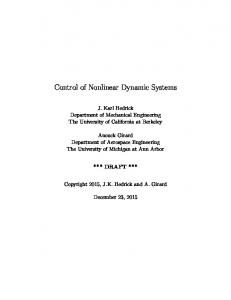
∥ˆ 𝑢 − 𝑢∗ ∥ ≤ 𝜀𝑢 , where 𝜀𝑢 = 12 ∥𝑅−1 ∥2𝐹 𝛽¯2 (𝑏2𝜃˜ + 𝜀2Δ𝑀 ). VI. S IMULATION AND C OMPARISON In this section, by an example, we illustrate the effectiveness of theorem 1 and design the optimal control for nonlinear systems (1). Now, we consider the following continuous-time nonlinear system 𝑥˙ = 𝐴 tanh(𝐾𝑥) + 𝑔(𝑥)𝑢, where [ ] [ ] 0.9373 −0.1135 −0.6636 0 𝐴= ,𝐾 = −5.3893 3.5724 0 −3.4946 ] [ and 𝑔(𝑥) = − sin(𝑥1 ) 0 . 𝑄 and 𝑅 in cost functional are identity matrices with appropriate dimensions. The objective is to find the control making 𝑥 converge to zero and minimize the (2). A. Simulation Now, by the theorem 1, we design the optimal control ] [ ] sech2 (𝑥1 ) 1[ 0 ˆ − sin(𝑥1 ) 0 𝜃. 𝑢∗ = − 0 sech2 (𝑥2 ) 2 We can see the evolution of 𝜃ˆ from Fig.1. After 110s, 𝜃ˆ converges to the ideal values, i.e. 𝜃ˆ = [−0.5073 0.3033]. The adjustable weights are reduced to two, (i.e. 𝜃ˆ1 and 𝜃ˆ2 ), for 2-order systems compared with the method of [10], [11]. The Fig.2 depicts the evolution of the system state under the control 𝑢∗ . Obviously, the state of the system is stable under the control 𝑢∗ .
0
50
100
Fig. 1.
150 Time (s)
200
250
300
Critic Parameters theta The states of the system
2 x1 x
1.5
2
1
x(t)
0.5 0 −0.5 −1 −1.5 −2
0
50
Fig. 2.
100
150 Time (s)
200
250
300
The states of the system
B. Comparison In this subsection, we simulate the results using the dualneural-network model method in [10]. Fig.3 shows evolution of the system states. We can see that the adjustable weight, (i.e. 𝑊𝑐 and 𝑊𝑎 ), converge to the ideal value (i.e. 𝑊𝑐 = [1.2278 0.1129 − 0.0253] and 𝑊𝑎 = [−0.6576 0.1100 0.7621], after 1500s, from Fig.4 and Fig.5. By the simulation, we can obtain the following results by comparing our method with dual-neural-network model method. ∙ Obviously, the convergence speed of the state and adjustable weights are slower than that of our method. ∙ For the 2-order system, only two adjustable weights are needed, while the dual-neural-network model needs six adjustable weights. When designing the control of high dimensional system, our method can reduce lots of the memory cells. VII. C ONCLUSION In this paper, we present a simple and effective scheme to design the optimal control for nonlinear systems. The FCE was
firstly employed to approximate the value function (i.e., the solution of the HJB equation). The advantages are to improve the previous approach, such as, reducing the storage space of updating weights, only using single model as approximator and enhancing the convergence speed. An example is used to prove the effectiveness and advantages of our approach.
The states of the system 2.5 x1 2
x
2
1.5 1 0.5 x(t)
VIII. ACKNOWLEDGEMENTS
0 −0.5 −1 −1.5 −2
0
500
Fig. 3.
1000 Time (s)
1500
2000
The states of the system
The authors would like to acknowledge the help from Zhiliang Wang and Xinrui Liu, currently an associate professor and lectorate at School of Information Science and Engineering, Northeastern University. This work was supported by the National Natural Science Foundation of China (50977008, 61034005, 61104010), the National High Technology Research and Development Program of China (2009AA04Z127), National Basic Research Program of China(2009CB320601), the Fundamental Research Funds for the Central Universities(N100404024). R EFERENCES
Parameters of the critic NN 3 Wc1 Wc2
2.5
Wc3 2
W1(t)
1.5 1 0.5 0 −0.5 −1
0
500
Fig. 4.
1000 Time (s)
1500
2000
Parameters of the critic NN
Parameters of the action NN 1 Wa1 W
a2
Wa3
0.5
W2(t)
0
−0.5
−1
−1.5
0
500
Fig. 5.
1000 Time (s)
1500
Parameters of the action NN
2000
[1] R. Beard, Improving the closed-loop performance of nonlinear systems, Ph.D. thesis, Rensselaer Polytechnic Institute, Troy, 1995. [2] R. Beard, G.N. Saridis and J.T. Wen, Galerkin approximations of the generalized Hamilton-Jacobi-Bellman equation, Automatica, vol.33, no.12, pp.2159–2177, 1997. [3] R. Beard, G.N. Saridis and J.T. Wen, Approximate solutions to the timeinvariant Hamilton-Jacobi-Bellman equation, Journal of Optimization Theory and Application, vol.96, no.3, pp.589–626, 1998. [4] G.N. Saridis and Chun-Sing G. Lee, An approximation theory of optimal control for trainable manipulators, IEEE Transactions on Systems, Man, Cybernetics, vol.9, no.3, pp.152–159, 1979. [5] D. Vrabie, O. Pastravanu and F.L. Lewis. Policy Iteration for ContinuousTime Systems with Unknown Internal Dynamics, Mediterranean Conference on Control and Automation, pp.1–6, June, Athens-Greece, 2007. [6] D. Vrabie and F.L. Lewis. Adaptive optimal control algorithm for continuous-time nonlinear systems based on policy iteration, Proceedings of the 47th IEEE Conference on Decision and Control Cancun, pp.73–79, Mexico, Dec, 2008. [7] D. Vrabie, O. Pastravanu, M. Abu-khalaf and F.L. Lewis. Adaptive optimal control for continuous-time linear systems based on policy iteration, Automatica, vol.45, no.2, pp.477–484, 2009. [8] D. Vrabie and F.L. Lewis. Neural network approach to continuous-time direct adaptive optimal control for partially unknown nonlinear systems, Neural Networks vol.22, no.3, pp.237–246, 2009. [9] M. Abu-Khalaf and F.L. Lewis, Nearly optimal control laws for nonlinear systems withsaturating actuators using a neural network HJB approach, Automatica, vol.41, no.5, pp.779–791, 2005. [10] K.G. Vamvoudakis and F.L. Lewis, Online actor-critic algorithm to solve the continuous-time infinite horizon optimal control problem, Automatica, vol.46, no.5, pp.878–888, 2010. [11] H. Zhang, L. Cui, X. Zhang and Y. Luo, Data-driven robust approximate optimal tracking control for unknown general nonlinear systems using adaptive dynamic programming method, IEEE Transactions on Neural Networks, vol.22, no.12, pp.2226–2236, 2011. [12] H. K. Khalil, Nonlinear Systems, Third Eidtion, Prentice Hall, December, 2001. [13] F.C. Chen and C.C. Liu, Adaptively controlling nonlinear continuoustime systems using multilayer neural networks, IEEE Transactions on Automatic Control, vol.39, no.6, pp.1306–1310, 1994. [14] T. Parisini and R. Zoppoli, Neural approximations for infinitehorizon optimal control of nonlinear stochastic systems, IEEE Transactions on Neural Network, vol.9, no.6, pp.1388–1408, 1998. [15] R.S. Sutton and A. G. Barto, Reinforcement learning:an introduction, Cambridge, MA: MIT Press, 1998. [16] B.A. Finlayson, The method of weighted residuals and variational principles, New York: Academic Press, 1990.
[17] M.T. Hagan, H.B. Demuth and M.H. Beale, Neural network design, PWS Pub, 1996. [18] W. M. Haddad and V. Chellaboina, Nonlinear dynamical systems and control: A Lyapunov-Based Approach Princeton, NJ: Princeton University Press, January, 2008. [19] D. V. Prokhorov and D. C. Wunsch, adaptive critic designs, IEEE Transactions on Neural Networks, vol.8, no.5, pp.997–1007, 1997. [20] D.E. Kirk, Optimal control theory-An introduction, New York: Dover Pub. Inc., Mineola, 2004. [21] K. Hornik, M. Stinchcombe and M. White, Universal approximation of an unknown mapping and its derivatives using multilayer feedforward networks, Neural Networks, vol.3, no.5, pp.551–560, 1990. [22] F.L. Lewis and V. Syrmos, Optimal Control, New York: Wiley, 1995. [23] J.J. Murray, C.J. Cox, G.G. Lendaris, and R. Saeks, Adaptive dynamic programming, IEEE Transactions on Systems., Man, Cybern., Part C: Appl. Rev., vol.32, no.2, pp. 140–153, 2002. [24] F.Y. Wang, N. Jin, D. Liu, and Q.Wei, Adaptive dynamic programming for finite-horizon optimal control of discrete-time nonlinear systems with -error bound, IEEE Transactions on Neural Network., vol.22, no.1, pp. 24–36, 2011. [25] H. Zhang, Q. Wei, and D. Liu, An iterative adaptive dynamic programming method for solving a class of nonlinear zero-sum differential games, Automatica, vol.47, no.1, pp. 207–214, 2011. [26] T. Dierks, B.T. Thumati, and S. Jagannathan, Optimal control of unknown affine nonlinear discrete-time systems using offline-trained neural networks with proof of convergence, Neural Network, vol.22, no.5-6, pp. 851–860, 2009. [27] H. Zhang, Y. Luo, and D. Liu, Neural-network-based near-optimal control for a class of discrete-time affine nonlinear systems with control constraints, IEEE Trans. Neural Netw., vol.20, no.9, pp.1490–1503, Sep. 2009 [28] J. Si, A.G. Barto, W.B. Powell, and D. Wunsch, Handbook of Learning and Approximate Dynamic Programming. New York: Wiley, 2004. [29] F.Y. Wang, H. Zhang, and D. Liu, Adaptive dynamic programming: An introduction, IEEE Comput. Intell. Mag., vol.4, no.2, pp.39–47, May 2009. [30] F.L. Lewis and D. Vrabie, Reinforcement learning and adaptive dynamic programming for feedback control, IEEE Circuits Syst. Mag., vol.9, no.3, pp.32–50, 2009. [31] A. Al-Tamimi, F.L. Lewis, and M. Abu-Khalaf, Model-free Q-learning designs for linear discrete-time zero-sum games with application to 𝐻∞ control, Automatica, vol.43, no.3, pp.473–481, 2007. [32] Y.H. Kim, F.L. Lewis and D.M. Dawson, Hamilton-Jacpbi-Bellman optimal design of functional lingk neural network controller for robot manipulators, Proceeding of the 36th Conference on Decision and Control, San Diego, California USA, 1997