Optimal Control of a Moving Boundary by Laser Heating in a 2-Phase Stefan Problem David Banks a,∗ , Xu Xu b , Rob Eason a , and Stephen Banks b a Optoelectronics b Department
Research Centre, University of Southampton, Southampton, SO17 1BJ, UK of Automatic Control and Systems Engineering, University of Sheffield, Mappin Street, Sheffield, S1 3JD, UK
Abstract The 2-phase heat control problem by a single laser point input is studied and a method of overcoming the moving boundary problem is introduced. This is achieved by applying a sequence of linear time varying control problems which converge to the single nonlinear problem which can be obtained from the joint moving boundary problems. Key words: Moving boundary problems, Linear time varying systems, Optimal control
Laser interactions with materials play a pivotal role in very many applications ranging from industrial scale cutting and welding, through to delicate surgery and machining of nanoscale features for microstructure manufacture. These applications have highly varied goals; for example, certain processes may require large amounts of material to be ablated per pulse, whilst others necessitate that laser-induced modification of the target is restricted to regions that may be sub-micron in size. The timescale on which the target reacts to the laser, for example phase front propagation velocities, can also be very important in determining the quality of the final result. For all of these processes, the common factor is that knowledge of how the target material reacts after irradiation with the laser is vital for accurate control of the result. Since the invention of the laser, such interactions have been studied extensively. These studies have been almost exclusively based around the resultant thermal processes in the target material given specified laser parameters. However, as most of the applications involving laser processing have relatively well-defined goals, it is apparent that a method ∗ Corresponding author Email addresses:
[email protected] (David Banks),
[email protected] (Xu Xu),
[email protected] (Rob Eason),
[email protected] (Stephen Banks). Preprint submitted to Elsevier
26 March 2008
where the desired modifications to the target are specified initially, and then a suitable laser input is calculated, would be a highly desirable tool. Recently we demonstrated a technique for determining an optimum control by classical methods for 2-phase heat diffusion (Stefan) problems (Banks, 2007). In this work we apply our technique to the situation of laser heating. A desired temperature profile within the target is specified and then the corresponding time-varying laser input required to obtain such a profile is calculated.
1. Background 1.1. Laser Temporal Control Temporal control of a processing laser beam is well-known to have significant effects on the subsequent thermal processes in the target. With the correct selection of the temporal profile, significant benefits can be achieved in many applications including micromachining (Dachraoui, 2006; Stoian, 2002), and cutting and welding (Simon, 1993). However, the determination of the optimal temporal form of the laser is a major challenge both experimentally and theoretically. The most common form of temporal control is to simply pulse the incident laser at a constant frequency, either by direct modulation of the laser source into a train of identical pulses (Simon, 1993) or by splitting a single incident pulse into multiple pulses, very closely spaced in time (Stoian, 2002). However, many techniques have been successfully demonstrated for modifying the temporal intensity distributions of lasers. Such techniques are readily available and are versatile enough to allow essentially arbitrary temporal waveforms to be generated. The effects of temporal pulse shaping of single pulses (Dachraoui, 2006) and pulse trains (Low, 2000) on the target material have received significant study. It is apparent from many of these studies that control of the temporal profile of the laser beyond simple pulsing is necessary to optimise the interaction with the target material. The difficulty with optimising a laser-matter interaction through temporal pulse shaping is that typically no prior knowledge of a suitable profile is available. To get around this difficulty, evolutionary algorithms are commonly employed to optimise the pulse shaping (Dachraoui, 2006). However this method can be relatively time-consuming, especially when no good “first guess” of the optimal profile is available. A further problem that can arise is that a quantifiable measure of the success of a particular pulse form may be hard to obtain in situ experimentally.
1.2. The Stefan Problem In this paper we consider the general 2-phase Stefan problem in a region Ω ⊆ 0, assuming constant thermal conductivity in each phase. The problem consists of two linear equations in unknown regions. In order to solve the problem, we show how to convert it into a single nonlinear diffusion equation with a temperature-dependant heat coefficient α(T ). To do this note that the classical Stefan boundary condition is given by h ∂T i+ ρLVn = − κ on ∂Γ1 , ∂n − where Vn is the velocity of the moving boundary, ρ is the density, L is the latent heat, κ is the thermal conductivity, and n is the normal to the phase boundary. The energy content in the liquid region is given by Z T L e (T ) = L + CL (T )dT , T > Tm Tm
and by
Z S
Tm
e (T ) =
CS (T )dT ,
T < Tm
T
where CL and CS are the respective specific heats. The corresponding conductivity coefficients (assuming the densities of each phase are equal and constant) are given by κS κL , αS (T ) = , αL (T ) = ρCL (T ) ρCS (T ) and the energy expressions can be unified by defining the specific heat Lδ(T − T ) + C (T ), T ≥ T m L m C(T ) = C (T ), T 0, and some finite t¯. Let y(t) = x(t) − xd (t) Then y(t) ˙ = x(t) ˙ − x˙ d (t) ¡ ¢ ¡ ¢ = f x(t), u(t) − f xd (t), ud (t) ¡ ¢ = g y(t), v(t), t where v(t) = u(t) − ud (t), and g(0, 0, t) = 0, by Taylor’s theorem. We can write this equation in the form ¡ ¢ ¡ ¢ y(t) ˙ = A y(t), v(t), t y(t) + B y(t), v(t), t v(t) for some matrix-valued functions A and B. Hence, we can always rewrite a tracking problem as a regular problem provided the system can track the desired function xd (t), i.e. there is an (open-loop) control ud (t) such that (12) holds. If xd is constant then (12) becomes f (xd , ud ) = 0
(11)
and so for trackability, there must exist a (constant) control ud such that (11) holds. Specialising to the heat control problem, if we want to track a given temperature profile T d , then we must have 7
d T1 α(T d ) −2α(T d ) α(T d ) 0 · · · · · · T2d 0 2 2 2 . .. .. .. .. .. .. .. .. . . . . . . . . 1 .. .................................................. (∆x)2 .. .................................................. . . .. .. .. .. .. .. .. . . . . . . . . . 0 ··· · · · · · · 0 α(TNd ) −2α(TNd ) TNd
−2α(T1d )
α(T1d )
0
··· ···
···
0
0 .. . 0 = − ... ud 0 .. . 0
Hence, if the input is in the mth place, we require α(T1d ) (−2T1d + T2d ) = 0 (∆x)2 α(T2d ) d (T − 2T2d + T3d ) = 0 (∆x)2 1 .. . d α(Tm−1 ) d d d (Tm−2 − 2Tm−1 + Tm )=0 2 (∆x) d ) d α(Tm d d (Tm−1 − 2Tm + Tm+1 ) = −ud 2 (∆x) .. .
α(TNd −1 ) (TN −2 − 2TN −1 + TN ) = 0 (∆x)2 α(TNd ) (TN −1 − 2TN ) = 0 (∆x)2 An elementary computation shows that Ti = iT1 , TN
Ti = (N − i + 1)TN , iT1 = N −i+1
and that ud =
α(Ti ) N + 1 T1 (∆x)2 N − i + 1
Hence, the only constant temperature profiles which are trackable are piecewise linear about the control point. In the case where we allow time-varying desired temperature profiles, Tid (t), we must satisfy the following equations: 8
T˙1d (t) + 2T1d (t) βT1d (t) T˙ d (t) T3d (t) = 2 d + 2T2d (t) − T1d (t) βT2 (t) ······ T˙ d (t) d d Tid (t) = i−1 + 2Ti−1 (t) − Ti−2 (t) d (t) βTi−1 T2d (t) =
(12)
and T˙Nd (t) + 2TNd (t) βTNd (t) T˙ d (t) TNd −2 (t) = Nd−1 + 2TNd −1 (t) − TNd (t) βTN −1 (t)
TNd −1 (t) =
······ d T˙i+1 (t) d d + 2Ti+1 (t) − Ti+2 (t) d (t) βTi+1
Tid (t) = ¢ ¡ ± where β = 1 (∆x)2 α(T ). To solve (12) we write
d Tk−1
Γk = Then the equations become
d Tk−1
Tkd
=
Tkd
0 1
d Tk−2 d Tk−1
−1 N
where N is the operator defined by N (T ) = Hence
d Tk−1
Tkd
=K
where
d Tk−2
0 1
Tkd
−1 N
d Tk−1
d Tk−1
K=
and so
1 dT β(T ) dt
= K k−2
Hence, 9
T1d T2d
(13)
T1d
Tid = K i−2 T˙ d (t) 1 d + 2T1 (t) d βT1 (t) 2 where (.)2 means the second component. Similarly, starting with (13) we have TNd Tid = K N −i−1 T˙ d (t) d N + 2T (t) N d βTN (t) 1 and so we have proved Theorem 3 A necessary and sufficient condition for the system (8) to be able to track a desired temperature profile is that (12) and (13) are satisfied and that T1 , and TN are related by TNd T1d N −i−1 d i−2 d T˙N (t) = K K T˙1 (t) d d + 2TN (t) + 2T1 (t) d (t) βT βT1d (t) N 2 1 moreover, the (open loop) control is given by d d ud = T˙id − β(Tid )(Ti−1 − 2Tid + Ti+1 ).
¤
Of course, for the case of laser heating we also have the condition that ud (t) ≥ 0
for all t ≥ 0
These conditions are highly nonlinear and can be used as a test for any given desired tracking. In general we will expect perfect tracking only for a very restricted class of functions. 4. Controlled Results Finally, we apply the model to a real problem. As an example, we consider the case of holding a 1D bar like that in fig. 2 at the melt temperature, i.e. Td (x, t) = Tm for all x and t. The parameters used were N = 30, l = 2, αL = 0.8, αS = 0.02, Tm = 0.25, and R = 0.5. The heating point was taken to be in the middle of the bar, i.e. m = 15, and the time step was δ = 0.001s. The initial condition was T [ i](x, 0) = 0. Figure 3 shows results obtained with 5 (fig. 3(a)) and 7 (fig. 3(b)) iterations. As can be seen the model again converged quickly, after around 5 iterations. Initially the control input was on, injecting heat into the bar and raising the temperature. It took just over 2.2 seconds for the heated region of the bar to reach the melting temperature (i.e. the desired condition), at which point the heat input was switched off and heat was allowed to diffuse in the bar. Due to the large difference in αL and αS heat diffused quickly out of the liquid regions, resulting in rapid solidification and an approximately flat-top temperature profile at around the melting temperature. However, limited diffusion in solid regions resulted in only minimal thermal diffusion following complete solidification and a temperature profile that only matched the desired profile close to the heating point. Continuing to run the simulation for longer time periods resulted in a oscillating solution where the heat input was turned on until the temperature was raised above the melt 10
7 iterations b)
5 iterations a) 0.5
0.5
0.25
T0.25
T 0 0.1
0 0.1
2
t
0 0
x
2
t
0.5
0 0
x
0.5
T
T
0.25
0.25
0 0.2
0 0.2
2
t
0.1 0
x
2
t
0.5
0.1 0
x
0.5
T
T
0.25
0.25
0 0.7
0 0.7
2
t
0.6 0
x
2
t
0.5
0.6 0
x
0.5
T
T
0.25
0.25
0 2.3
2
t
2.2 0
x
11
0 2.3
2
t
2.2 0
x
Fig. 3. Plots of the solution of the controlled system using 5 (a) and 7 (b) iterations.
temperature, and then off until sufficient diffusion occurred that the bar cooled below Tm . Heat diffusion in the lateral direction was limited by the small αS so the temperature profile closely matched the desired condition only close to the heating point. Better tracking of the desired condition was achievable by reducing αL /αS . 5. Conclusions We have shown how to approximate a nonlinear controlled Stefan problem using a linearisation technique. The method allows for the tracking of desired temperature profiles within targets heated by an external heat source, e.g. a laser. References D.P. Banks, R.W. Eason, and S.P. Banks, “Control of Phase Boundary in a 2-Phase Stefan Problem by Laser Heating,” 8th International Carpathian Control Conference ˇ (ICCC), Strbsk´ e Pleso, Slovakia (2007). H. Dachraoui and W. Husinsky, “Thresholds of plasma formation in silicon identified by optimizing the ablation laser pulse form,” Phys. Rev. Lett. 97, 107601-1 – 4 (2006). R. Stoian, M. Boyle, A. Thoss, A. Rosenfeld, G. Korn, I.V. Hertel, and E.E.B. Campbell, “Laser ablation of dielectrics with temporally shaped femtosecond pulses,” Appl. Phys. Lett. 80(3), 353-355 (2002). G. Simon, U. Gratzke, and J. Kroos, “Analysis of heat conduction in deep penetration welding with a time-modulated laser beam,” J. Phys. D: Appl. Phys. 26, 862-869 (1993). M. Tomas-Rodriguez, and S.P. Banks, “Linear Approximations to Nonlinear Dynamical Systems with Applications to Stability and Spectral Theory,” IMA J. Math. Cont Inf., 20, 89-104 (2003). D.K.Y. Low, L. Li, and P.J. Byrd, “Combined Spatter and Hole Taper Control in Nd:YAG Laser Percussion Drilling,” 19th International Congress on Applications of Lasers and Electro-Optics (ICALEO) 2000, Section B, 11 – 20.
12