Optimal Design of the Double Sampling X Chart ... - Semantic Scholar

International Journal of Chemical Engineering and Applications, Vol. 3, No. 5, October 2012

Optimal Design of the Double Sampling X Chart Based on Median Run Length Wei Lin Teoh and Michael B. C. Khoo

sample sizes, ASS0 ∈ {3, 5, 7, 9}. These optimal parameters

concluded that the DS X chart has a better performance in certain cases. In light of this advantage, recently, Torng et al. [4], Irianto and Juliani [5], Costa and Machado [6], Khoo et al. [7], and Lee et al. [8], to name a few, contributed to the area of DS control charts. The sole dependence on the average run length (ARL) as a measure of a chart’s performance has been subjected to criticism in recent years (see [9]-[11]). Since the skewness of the run length distribution changes from highly skewed when the process is in-control to approximately symmetric when the process mean shift is large, interpretation based on ARL alone could be misleading. For instance, the DS X chart with ( n1 = 1, n2 = 5, L1 = 0.253, L = 5.046, L2 = 3.067) has

facilitate the implementation of the DS X chart in practice.

an in-control ARL ( ARL0 ) of 500, where the notations ( n1 ,

Abstract—The double sampling (DS) X chart is effective in detecting small to moderate process mean shifts and reducing the sample size. The average run length (ARL) is an intuitively appealing and widely used optimization criterion in the design of a control chart. Nevertheless, the skewness of the run length distribution changes with the size of the process mean shift; thus, ARL is not necessarily a good representative of the run length distribution. In such a case, the median run length (MRL) provides a more reliable interpretation, for the in-control and out-of-control performances of a control chart. In this paper, an optimal design of the DS X chart based on MRL is proposed. New optimal parameters are provided for selected in-control median run lengths, MRL0 ∈ {250, 500} and in-control average

n2 , L1 , L , L2 ) of the DS X chart are defined in Section II.

Index Terms—Average sample size, double sampling X chart, median run length, optimization.

However, it is found that 50% of all the run lengths are less than 347 (i.e. the in-control median run length, MRL0 = 347) and about 63% of all the run lengths are less than 500. In view of this disadvantage, Chakraborti [10] pointed out that the median run length (MRL) provides a more accurate measure of a chart’s performance. For example, the DS X chart with the parameters stated above has an out-of-control MRL ( MRL1 ) of 23 at shift δ = 0.5. This indicates that in 50% of the time, the out-of-control run length is less than or equal to 23 samples. Note that all the MRLs and the percentage point of the run length distribution are calculated by using the formulae shown in Section II. In short, interpretation based on MRL is more readily comprehended. Therefore, MRL is suggested as an alternative performance criterion to design control charts. For related literatures, see Gan [12]-[13], Maravelakis et al. [14], Golosnoy and Schmid [15], Low et al. [16], and Khoo et al. [17].

I. INTRODUCTION Contemporarily, the quality of the final products and customers’ satisfaction are vitally viewed in the manufacturing and service processes, such as in the chemical industries, food industries and health care services. Statistical Process Control (SPC) is a collection of statistical tools that provide improvement in yield and reduction in production costs. A control chart is one of the most valuable tools in SPC to reduce variability in key parameters and produce conforming products. Because of the operational simplicity, the Shewhart X chart is extensively used to detect large process mean shifts in industries. However, it is relatively insensitive in detecting small and moderate process mean shifts. To overcome this problem, Daudin [1] applied the concept of double sampling plans to propose the DS X chart, which is viewed as a two-stage Shewhart X chart. The optimization model to minimize the in-control average sample size ( ASS0 ) is presented in Daudin’s [1] paper. From the statistical viewpoint, Irianto and Shinozaki [2] constructed an optimization model to minimize the out-of-control average run length ( ARL1 ). Daudin [1] and Costa [3] compared the performances of the DS X chart with the Shewhart, EWMA, CUSUM, variable sampling interval (VSI) and variable sample size (VSS) charts. They

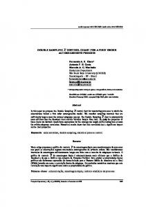
Fig. 1. Graphical view of the DS X control chart’s operation.

This paper is structured as follows: First, Section II briefly introduces the DS X chart and its run length properties. Since MRL can increase the quality control engineers’ confidence in understanding a control chart, the main contributions of this paper are to propose an optimization

Manuscript received August 12, 2012; revised September 23, 2012. This research is supported by the Universiti Sains Malaysia, Incentive-Postgraduate Grant, no, 1001/PMATHS/822080. The authors are with the School of Mathematical Sciences, Universiti Sains Malaysia, and 11800 Penang, Malaysia (e-mail: [email protected], [email protected]).

DOI: 10.7763/IJCEA.2012.V3.205

303


500} and ASS0 ∈ {3, 5, 7, 9}, which are presented in Section III. Conclusions are drawn in Section IV.

model for the DS X chart by minimizing MRL1 and provide specific optimal combinations for MRL0 ∈ {250,

TABLE I: OPTIMAL ( n1 , n2 , L1 , L , L2 ) COMBINATION (FIRST ROW OF EACH CELL) AND ( MRL1 , ASS1 ) VALUES (SECOND ROW OF EACH CELL) OF THE DS X CHART WHEN MRL0 ∈ {250, 500}, ASS0 ∈ {3, 5, 7, 9} AND δ opt ∈ {0.2, 0.4, 0.6, 0.8, 1.0, 1.2, 1.4, 1.6, 1.8, 2.0}

MRL0 = 250

δ opt

ASS0 = 3

ASS0 = 5

ASS0 = 7

ASS0 = 9

0.2

(1, 14, 1.465, 4.093, 2.527) (70, 3.111) (1, 14, 1.464, 3.608, 2.565) (17, 3.437) (1, 13, 1.426, 3.875, 2.567) (6, 3.930) (1, 11, 1.335, 3.894, 2.635) (3, 4.429) (1, 7, 1.066, 3.481, 2.853) (2, 4.404) (2, 6, 1.382, 3.748, 2.842) (1, 5.626) (1, 4, 0.674, 3.999, 2.934) (1, 4.121) (1, 3, 0.430, 3.400, 3.046) (1, 3.593) (1, 3, 0.430, 3.400, 3.046) (1, 3.618) (1, 3, 0.430, 3.400, 3.046) (1, 3.606)

(3, 12, 1.383, 4.186, 2.775) (59, 5.302) (2, 13, 1.198, 4.063, 2.761) (12, 5.928) (2, 12, 1.150, 3.756, 2.803) (4, 6.831) (1, 13, 1.020, 3.692, 2.763) (2, 6.793) (3, 7, 1.066, 3.481, 2.976) (1, 7.967) (1, 6, 0.430, 3.600, 2.975) (1, 5.936) (3, 3, 0.430, 3.400, 3.051) (1, 5.443) (3, 3, 0.430, 3.400, 3.051) (1, 5.179) (3, 3, 0.430, 3.400, 3.051) (1, 4.824) (3, 3, 0.430, 3.400, 3.051) (1, 4.420)

(5, 10, 1.282, 4.513, 2.904) (54, 7.440) (6, 9, 1.593, 4.025, 2.885) (10, 8.464) (3, 12, 0.967, 3.537, 2.928) (3, 9.542) (1, 10, 0.524, 4.217, 2.900) (2, 8.010) (1, 10, 0.524, 4.217, 2.900) (1, 8.459) (5, 3, 0.430, 3.400, 3.039) (1, 7.256) (5, 3, 0.430, 3.400, 3.039) (1, 6.809) (5, 3, 0.430, 3.400, 3.039) (1, 6.286) (4, 4, 0.318, 3.413, 3.048) (1, 5.701) (4, 4, 0.318, 3.413, 3.048) (1, 5.114)

(4, 11, 0.748, 4.268, 2.947) (53, 9.384) (2, 13, 0.615, 4.373, 2.905) (10, 9.788) (2, 13, 0.615, 3.908, 2.914) (3, 10.617) (4, 11, 0.748, 3.714, 2.966) (1, 12.747) (6, 4, 0.318, 3.413, 3.039) (1, 9.274) (6, 4, 0.318, 3.413, 3.039) (1, 8.713) (6, 4, 0.318, 3.413, 3.039) (1, 7.970) (5, 5, 0.253, 3.419, 3.047) (1, 7.182) (5, 5, 0.253, 3.419, 3.047) (1, 6.361) (4, 6, 0.210, 3.422, 3.052) (1, 5.689)

0.4 0.6 0.8 1.0 1.2 1.4 1.6 1.8 2.0

MRL0 = 500

δ opt

ASS0 = 3

ASS0 = 5

ASS0 = 7

ASS0 = 9

0.2

(2, 13, 1.769, 4.329, 2.771) (117, 3.154) (2, 13, 1.769, 4.136, 2.776) (23, 3.613) (2, 13, 1.769, 4.136, 2.776) (7, 4.375) (2, 13, 1.769, 4.136, 2.776) (3, 5.413) (1, 10, 1.282, 4.558, 2.908) (2, 5.002) (2, 9, 1.593, 4.158, 2.934) (1, 6.815) (1, 5, 0.842, 4.459, 3.107) (1, 4.615) (1, 4, 0.674, 3.972, 3.160) (1, 4.301) (1, 3, 0.430, 3.585, 3.255) (1, 3.671) (1, 3, 0.430, 3.585, 3.255) (1, 3.678)

(3, 12, 1.383, 4.307, 3.020) (100, 5.302) (3, 12, 1.383, 4.307, 3.020) (17, 6.166) (2, 13, 1.198, 3.844, 3.024) (5, 6.970) (2, 12, 1.150, 3.921, 3.039) (2, 8.014) (3, 9, 1.220, 3.598, 3.171) (1, 8.997) (1, 7, 0.566, 4.188, 3.131) (1, 6.420) (1, 5, 0.253, 3.603, 3.249) (1, 5.548) (3, 3, 0.430, 3.585, 3.257) (1, 5.349) (3, 3, 0.430, 3.585, 3.257) (1, 5.029) (3, 3, 0.430, 3.585, 3.257) (1, 4.641)

(5, 10, 1.282, 4.558, 3.132) (93, 7.440) (6, 9, 1.593, 4.158, 3.121) (15, 8.467) (3, 12, 0.967, 3.715, 3.152) (4, 9.570) (1, 13, 0.736, 3.896, 3.074) (2, 8.627) (2, 9, 0.589, 4.125, 3.155) (1, 9.330) (5, 3, 0.430, 3.585, 3.246) (1, 7.416) (5, 3, 0.430, 3.585, 3.246) (1, 7.016) (5, 3, 0.430, 3.585, 3.246) (1, 6.506) (5, 3, 0.430, 3.585, 3.246) (1, 5.989) (4, 4, 0.318, 3.597, 3.254) (1, 5.373)

(8, 7, 1.465, 4.224, 3.180) (91, 9.436) (8, 7, 1.465, 4.224, 3.180) (14, 10.611) (2, 13, 0.615, 4.069, 3.132) (4, 10.623) (1, 12, 0.430, 3.585, 3.207) (2, 10.010) (1, 11, 0.348, 3.594, 3.221) (1, 10.094) (6, 4, 0.318, 3.597, 3.245) (1, 8.963) (6, 4, 0.318, 3.597, 3.245) (1, 8.263) (6, 4, 0.318, 3.597, 3.245) (1, 7.494) (5, 5, 0.253, 3.603, 3.252) (1, 6.682) (5, 5, 0.253, 3.603, 3.252) (1, 5.961)

1) Take a first sample of size

n1 and compute the sample

0.4 0.6 0.8 1.0 1.2 1.4 1.6 1.8 2.0

II. THE DS X CHART

X 1i = ∑ j1=1 X 1i , j n1 n

It is assumed that the observations of the quality characteristic X are independently and identically distributed (iid) normal random variables, with an in-control mean μ0

mean

, where

X 1i , j

with

j = 1, 2, ...,

n1 is the jth observation in the ith sampling time of the first sample.

and an in-control variance σ 0 2 . Let L1 and L be the warning and control limits of the first sample, respectively; whereas L2 be the control limit of the combined samples. The regions

Z = ⎡( X − μ

)

n ⎤ σ 0 ∈ I1

1i 0 1⎦ ⎣ 1i 2) If considered as in-control.

in Fig. 1 are represented as I1 = [ − L1 , L1 ] , I 2 = [ − L, − L1 )

, the process is

∪ ( L1 , L ] , I 3 = ( −∞, − L ) ∪ ( L, + ∞ ) , and I 4 = [ − L2 , L2 ] .

3) If

Z1i ∈ I 3 , the process is concluded as out-of-control.

By referring to Fig. 1, the design procedure of the DS X chart demonstrated by Daudin [1] is as follows:

4) If

Z1i ∈ I 2 , take a second sample of size n2 and calculate X 2i = ∑ j2=1 X 2i , j n2 n

the sample mean 304

, where

X 2i , j


j=

where

n

with 1, 2, ..., 2 is the jth observation in the ith sampling time of the second sample.

(

mean

X i = ( n1 X 1i + n2 X 2i )

)

(

)

P ( Z1i ∈ I 2 ) = Φ L + δ n1 − Φ L1 + δ n1 +

5) At the ith sampling time, calculate the combined-sample

(

( n1 + n2 ) .

)

(

)

Φ − L1 + δ n1 − Φ − L + δ n1 .

(6)

Z i = ⎡( X i − μ0 ) n1 + n2 ⎤ σ 0 ∈ I 4

⎣ ⎦ 6) If , the process is declared as in-control; otherwise, it is deemed as out-of-control.

III. OPTIMAL DESIGN OF THE DS X CHART BASED ON MRL In this paper, the performance of the DS X chart is evaluated, in terms of the MRL and ASS. When the process is in-control, the MRL is denoted as MRL0 ; while the

Note that the ith sampling time refers to the ith time when either the first sample of size n1 only or the combined samples of size n1 + n2 , respectively are collected.

out-of-control MRL is denoted as MRL1 . Similarly, two ASSs are usually of interest, namely the in-control ASS, ASS0 and the out-of control ASS, ASS1 . In this section, an

It is further assumed that μ0 and σ 0 2 is known. Let Pak be the probability that the process is regarded as in-control at stage k with k ∈ {1, 2}. Then Pa = Pa1 + Pa 2 is the probability of the in-control process, with (see [1]) Pa1 = P ( Z1i ∈ I1 )

(

)

(

)

= Φ L1 + δ n1 − Φ − L1 + δ n1 ,

and

optimal design of the DS X chart for minimizing MRL1 (δ opt ) is developed. Here, δ opt represents the size of a process mean shift, for which a quick detection is required. It is noted that when MRL0 , ASS0 and δ are fixed, a control chart is considered superior to its competitors if it has the smallest MRL1 value. Similarly, a DS X chart, for optimally detecting a desired shift is obtained when the optimal parameters giving the lowest MRL1 , are identified

(1)

Pa 2 = P ( Z i ∈ I 4 and Z1i ∈ I 2 ) =∫

z∈I 2*

⎡ ⎛ n ⎞ ⎢Φ ⎜⎜ cL2 + rcδ − 1 z ⎟⎟ − n2 ⎠ ⎣⎢ ⎝

from all the possible ( n1 , n2 , L1 , L , L2 ) combinations. The proposed optimization model is illustrated as follows:

⎛ n ⎞⎤ Φ ⎜⎜ −cL2 + rcδ − 1 z ⎟⎟ ⎥ φ ( z ) dz , n2 ⎠ ⎦⎥ ⎝

(2)

Min

n1 , n2 , L1 , L , L2

where Φ (. ) and φ (. ) are the cumulative distribution

MRL0 = τ ,

(L +δ

and

ASS0 = n,

)

I 2* = ⎡⎣ − L + δ n1 , − L1 + δ n1 ∪

(9)

where n is the expected in-control average sample size;

n1 , L + δ n1 ⎤⎦ . Note that a run length (RL) is the number of samples taken before the chart signals the first out-of-control condition. Montgomery [18] pointed out that the run length distribution of a Shewhart chart is the geometric distribution. It is known that the DS X chart is a Shewhart type chart; thus, all the run length properties of the DS X chart can be characterized by the geometric distribution. Hence, the cdf of RL, i.e. FRL ( A )

1 ≤ n1 < n < n1 + n2 ≤ nmax ,

1

(10)

where nmax is the upper bound of n1 + n2 . A nonlinear optimization algorithm is employed to determine the optimal ( n1 , n2 , L1 , L , L2 ) combination for each case considered in this paper. Practically, either a small or a moderate sample size is adopted in industry; thus, nmax = 15 is set in this paper. It must be emphasized that MRL is an integer due to the discrete property of RL; hence, there may exist several optimal ( n1 , n2 , L1 , L , L2 ) combinations

is obtained as FRL ( A ) = P ( RL ≤ A ) = 1 − Pa A ,

(8)

where τ is the expected in-control median run length;

shift with the out-of-control mean μ1 , r = n1 + n2 , n2

(7)

Subject to

function (cdf) and probability density function (pdf) of the standard normal random variable, respectively. Here, δ = μ0 − μ1 σ 0 is the magnitude of the standardized mean c=r

MRL1 (δ opt ) ,

(3)

for which the MRL1 value is minimum at a specific δ opt ≠ 0.

where A ∈ {1, 2, 3, ...}. Then the MRL of the DS X chart is equal to (see [12] and [13])

In such a case, the DS X chart with the optimal ( n1 , n2 , L1 ,

P ( RL ≤ MRL − 1) ≤ 0.5 and P ( RL ≤ MRL ) > 0.5.

Daudin [1] also showed that the average sample size (ASS) at each sampling time is equal to

The optimal ( n1 , n2 , L1 , L , L2 ) combinations and their corresponding ( MRL1 , ASS1 ) values for different combinations of MRL0 , ASS0 and δ opt , are presented in the

ASS = n1 + n2 P ( Z1i ∈ I 2 ) ,

first and second rows of each cell in Table I, respectively. The above proposed optimization model (7)-(10) is applied

L , L2 ) combination having the smallest ASS1 is preferred.

(4)

(5)

305


here to obtain the optimal ( n1 , n2 , L1 , L , L2 ) combinations. It must be accentuated that MRL0 = τ ∈ {250, 500} (constraint (8)) and ASS0 = n ∈ {3, 5, 7, 9} (constraint (9)) are attained for each case shown in Table I. The results in Table I have been verified with simulation. These new optimal ( n1 , n2 , L1 , L , L2 ) combinations facilitate the implementation of the DS X chart in practice. For example, consider a continuous chemical process in which a quick detection is desired at a shift with magnitude δ opt = 1.0. If

proposed the DS X chart, optimized based on the ARL. Furthermore, specific optimal charting parameters, based on MRL are provided to aid practitioners in implementing the DS X chart instantaneously. REFERENCES [1] [2]

MRL0 = 250 and ASS0 = 5 are selected, Table I suggests using ( n1 = 3, n2 = 7, L1 = 1.066, L = 3.481, L2 = 2.976) as the optimal parameters to detect such a shift. Additionally, Table I tells us that 50% of the time, a shift with magnitude δ = 1.0 is detected by the first sample (i.e. MRL1 = 1). Also, the chart needs 7.967 observations on the average to detect such a shift. The choice of MRL0 primarily depends on the rate of production and the rate of sampling. Accordingly, two MRL0 s are considered in this paper, i.e. MRL0 ∈ {250, 500}. Examination of Table I reveals that a large MRL0 issues false alarms less frequently than a small MRL0 ; however, the latter responds quicker to an out-of-control condition, especially for a small δ opt . As expected, the

[3] [4]

[5]

[6]

[7]

[8]

[9]

sensitivity of the DS X chart in detecting a particular shift increases as ASS0 increases. This improvement is more pronounced for small δ opt . It is interesting to note that for

[10]

moderate and large shifts ( δ opt ≥ 1.2), the DS X chart has

[11]

the same minimum MRL1 value regardless of the ASS0 used. Daudin [1] stated that the DS chart is designed, where the sample size should be increased if there is a higher chance of inferior quality. Therefore, it is observed that for most of the cases in Table I, the ASS1 taken to detect an out-of-control situation is higher than the corresponding ASS0 . Apparently, some of the optimal ( n1 , n2 , L1 , L , L2 ) combinations are optimally detecting a range of shifts. For instance, when MRL0 = 500 and ASS0 = 7, the optimal ( n1 = 5, n2 = 3, L1 = 0.430, L = 3.585, L2 = 3.246) combination is optimally detecting the shifts in the range 1.2 ≤ δ opt ≤ 1.8. This is a favorable property of the DS X

[14]

chart, optimized based on MRL, as it is sometimes difficult to predict the actual process mean shift in practice.

[17]

[12]

[13]

[15]

[16]

[18]

IV. CONCLUSION A good understanding of the control charts used is crucial to engineers and shop floor personnel. Since the run length distribution changes in accordance to the magnitude of mean shifts, the MRL is more readily interpreted than the ARL. Moreover, the MRL provides more credible information for practitioners. This paper demonstrates the optimization design of the DS X chart, based on MRL and thus, complements the work of Irianto and Shinozaki [2], who

J. J. Daudin, “Double sampling X charts,” Journal of Quality Technology, vol. 24, pp. 78-87, 1992. D. Irianto and N. Shinozaki, “An optimal double sampling X control chart,” International Journal of Industrial Engineering – Theory, Applications and Practice, vol. 5, pp. 226-234, 1998. A. F. B. Costa, “ X charts with variable sample size,” Journal of Quality Technology, vol. 26, pp. 155-163, 1994. C. C. Torng, P. H. Lee, and N. Y. Liao, “An economic-statistical design of double sampling X control chart,” International Journal of Production Economics, vol. 120, pp. 495-500, 2009. D. Irianto and A. Juliani, “A two control limits double sampling control chart by optimizing producer and customer risks,” ITB Journal of Engineering Science, vol. 42, pp. 165-178, 2010. A. F. B. Costa and M. A. G. Machado, “Variable parameter and double sampling X charts in the presence of correlation: The Markov chain approach,” International Journal of Production Economics, vol. 130, pp. 224-229, 2011. M. B. C. Khoo, H. C. Lee, Z. Wu, C. H. Chen, and P. Castagliola, “A synthetic double sampling control chart for the process mean,” IIE Transactions, vol. 43, pp. 23-38, 2011. P. H. Lee, Y. C. Chang, and C. C. Torng, “A design of S control charts with a combined double sampling and variable sampling interval schem,” Communications in Statistics – Theory and Methods, vol. 41, pp. 153-165, 2012. F. F. Gan, “Exact run length distributions for one-sided exponential CUSUM schemes,” Statistical Sinica, vol. 2, pp. 297-312, 1992. S. Chakraborti, “Run length distribution and percentiles: The Shewhart X chart with unknown parameters,” Quality Engineering. vol. 19, pp. 119-127, 2007. M. B. C. Khoo, V. H. Wong, W. Zhang, and P. Castagliola, “Optimal designs of the multivariate synthetic chart for monitoring the process mean vector based on median run length,” Quality and Reliability Engineering International, vol. 27, pp. 981-997, 2011. F. F. Gan, “An optimal design of EWMA control charts based on median run length,” Journal of Statistical Computation and Simulation, vol. 45, pp. 169-184. 1993. F. F. Gan, “An optimal design of cumulative sum control chart based on median run length,” Communications in Statistics – Simulation and Computation, vol. 23, pp. 485-503, 1994. P. E. Maravelakis, J. Panaretos, and S. Psarakis, “An examination of the robustness to non normality of the EWMA control charts for the dispersion,” Communications in Statistics – Simulation and Computation, vol. 34, pp. 1069-1079, 2005. V. Golosnoy and W. Schmid, “EWMA control charts for monitoring optimal portfolio weights,” Sequential Analysis, vol. 26, pp. 195-224, 2007. C. K. Low, M. B. C. Khoo, W. L. Teoh, and Z. Wu, “The revised m-of-k runs rule based on median run length,” Communications in Statistics – Simulation and Computation, vol. 41, pp. 1463-1477, 2012. M. B. C. Khoo, V. H. Wong, Z. Wu, and P. Castagliola, “Optimal design of the synthetic chart for the process mean based on median run length,” IIE Transactions, In press. D. C. Montgomery, Statistical quality control: A modern introduction, 6th ed, New York: John Wiley and Sons, 2009.

Wei Lin Teoh is a Ph.D. student in the School of Mathematical Sciences, Universiti Sains Malaysia (USM). She received her Bachelor of Science with Education (Honours) in Mathematics from USM in 2010. Michael B.C. Khoo is a Professor in the School of Mathematical Sciences, Universiti Sains Malaysia (USM). He received his Ph.D. in Applied Statistics in 2001 from USM. He specializes in Statistical Process Control. He is a member of the American Society for Quality and serves as a member of the editorial boards of several international journals.

306