Optimal Load Shedding Using an Ensemble of Artificial Neural Networks

Optimal Load Shedding Using an Ensemble of Artificial Neural Networks Original Scientific Paper Muhammad FaizanTahir [email protected]

Hafiz Teheeb-Ul-Hassan [email protected]

Kashif Mehmood [email protected]

The University of Lahore, Faculty of Electrical Engineering, Department of Engineering 1 Km Defence Road, Lahore, Pakistan

Hafiz Ghulam Murtaza Qamar [email protected]

Umair Rashid [email protected] Abstract – Optimal load shedding is a very critical issue in power systems. It plays a vital role, especially in third world countries. A sudden increase in load can affect the important parameters of the power system like voltage, frequency and phase angle. This paper presents a case study of Pakistan’s power system, where the generated power, the load demand, frequency deviation and load shedding during a 24-hour period have been provided. An artificial neural network ensemble is aimed for optimal load shedding. The objective of this paper is to maintain power system frequency stability by shedding an accurate amount of load. Due to its fast convergence and improved generalization ability, the proposed algorithm helps to deal with load shedding in an efficient manner.

Keywords – ensemble of artificial neural network, load shedding, power system stability

1. INTRODUCTION In this modern era, power consumption is increasing extensively with each passing day. A growing population with the need of more new plazas and buildings is responsible for greater energy consumption. An increase in power demand requires construction of more and more grids, and third world countries do not have enough resources to cope with this problem. The method to deal with this problem in order to gain system stability is to shed some load. This process is known as load shedding. Optimal load shedding is defined as the curtailment of minimum load for each subsystem so that poise of demand and supply remain conserve [1]. When the load increases, generators connected to the power system slow down results in frequency decay. The threshold frequency value in Pakistan is 49.5 Hz. A decrease in frequency below the threshold value results in shutting down the generators. The shutting down of a generator in an interconnected system can trigger the failure of other parallel generators. This condition is known as a cascaded failure or blackout [2]. Volume 7, Number 2, 2016

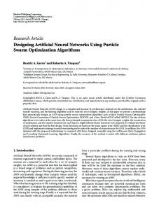
The case when system generation is greater than system demand causes the frequency to rise up [1]. An increase in frequency above the threshold value results in speeding up the generator until it burns out as shown in Figure 1.

Fig. 1. Relation of frequency with generation and demand When the load increases, the first action is performed by the governor that adjusts the speed by increasing the fuel quantity to recover the slow speed of the machine. In the case when the governor is not able to com-

39

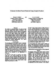
pensate for declining frequency, load shedding is the final and ultimate solution [3]. There are several ways to shed load, like the breaker interlock method, under the frequency relay and programmable logic controller [4]. The disadvantages of these methods are that they are too slow and not highly efficient when disturbances and losses in the system are included during real-time calculation of load [5]. Many algorithms have been applied for optimal load shedding for maintaining the steady state of the power system. Results obtained by traditional methods take more time as compared to artificial neural networks (ANN) [6]. This method can determine the amount of load shedding magnitude in each step simultaneously that leads to a higher speed than traditional methods [5]. The error in the learning of an artificial neural network can be reduced by ensembling neural networks which will increase the accuracy of the system [7]. Optimal load shedding using an artificial neural network ensemble is the outcome of this research. In this paper, the Bootstrap Aggregating (Bagging) algorithm with Disjoint Partition is used to ensemble an ANN because of its fast convergence and low variance [8]. 2. RELATED WORK The basic idea of an ANN comes from the biological nervous system. ANNs are considered to be a simplified model of a biological neural network. ANNs are trained so that a specific input leads to a specific output target. It has to be trained to find a nonlinear relation between an input and an output. The basic layout of an ANN consists of an input layer, a hidden layer and an output layer. The first step in designing the ANN is to find out the architecture that will yield best possible results. The size of the hidden layer is mostly 10% of the input layer [9]. Data transmission from the input layer to the output layer is shown in Figure 2.

value is determined by the type of the transfer function. The summation function is compared with the threshold value; if the sum is greater than this threshold value, the output signal will be activated and vice versa. The desired output is compared with the ANN output and the difference between these two outputs is called error. The error is propagated backward to adjust the input weights in order to match the neural output with the desired one. Nakawiro et al. [10] proposed the Ant Colony Optimization (ACO) technique for optimal load shedding. In this algorithm, the authors achieved load shedding by observing load variation at various buses by voltage stability margin; ACO will decide which load of which particular bus will be shed. A high speed makes this technique superior to other conventional methods. The shortcoming of this technique is its high complexity and convergence time is very high. Chawla et al. [11] proposed a genetic algorithm (GA) for optimal load shedding. In this algorithm, load shedding is used to prevent voltage stability. A power world simulator is used to analyze the continuation of the power flow that helps determine load shedding. The GA will decide how much load will be shed at each bus. This algorithm is very easy to understand and it does not require much knowledge of mathematics. The shortcoming of this algorithm is the occurrence of data overfitting and it is too slow for real-time cases where long training is required. 3. ENSEMBLE OF ARTIFICIAL NEURAL NETWORK An Ensemble of Artificial Neural Networks (EANN) consists of a number of ANN networks and an algorithm for combining their outputs [9]. Each individual network has a different input data set but the same target data set. After being combined and processed by the algorithm, the outputs of neural networks give the final EANN output.

Fig. 2. Activation and flow of information in an ANN Each of the ANN inputs has a specified weight which is indicated by w0, w1 and w2, respectively. These weights are the strength of inputs and they determine the intensity of the input signal. The summation function decides how inputs and their weights are combined. Sometimes an activation function or bias is added in order to get the threshold value. The threshold

40

Fig. 3. Artificial neural network ensemble

International Journal of Electrical and Computer Engineering Systems

There are many algorithms to ensemble ANNs [12]. In this research, Bootstrap Aggregating (Bagging) is used to ensemble ANNs. This algorithm depends on majority voting and different classifiers are combined by taking their means as shown in Figure 4:

between the actual and the target output is called error. The reason for this error lies in the learning process. Three main factors of errors in learning are bias, variance and noise [6].

Error=Noise+ Bias+ Variance

(1)

Large bias causes underfitting of data, while high variance causes overfitting of data [8]. Compared to a single classifier, grouping of classifiers may teach a more expressive concept class resulting in the reduction of bias [14], [15]. Results are relatively less dependent on a single training data set that results in variance reduction. Generalization of data to opt new data will increase when bias and variance are cut to a minimum and data will not suffer from over- and underfitting. 5. THE PROPOSED METHOD The procedure to be adopted in this scenario has the following three steps:

Fig. 4. General idea of bagging Bagging is classified in two ways, i.e.; i) small bags, and ii) disjoint partition [13]. The small bags algorithm works such that subsets of the original data set may not be equal to the original data set. A disadvantage of small bags is the probability of repeating the number more than once. Disjoint partition makes the subsets of original data sets such that the number of the subset shall be equal to the original data set. Disjoint partition is considered to be more effective and accurate compared to small bags [13], [14]. The original data set is shown in Figure 5:

Fig. 5. Original data set In a disjoint partition case, each particular number from the original data set is selected such that no repetition occurs, as shown in Figure 6:

Fig. 6. Disjoint partition 4. PROBLEM MOTIVATION It is well-known that prediction can be improved by combining results of several predictors. In comparison to ANNs, EANNs always improve the results. EANN prediction will only be incorrect when the majority of ANN prediction data sets proves to be wrong. If the majority of prediction of ANNs proves to be wrong, then there is a problem in the data set [7, 15]. The output of an ANN does not match with the target function even after several trainings. The difference Volume 7, Number 2, 2016

1. Real data set generation, 2. Design of an ANN, 3. Design of an EANN. Step 1: In this paper, a real-data set of one complete day of the Water and Power Development Authority (WAPDA), Pakistan, has been used. Data is provided by the National Power Control Centre (NPCC) Islamabad that monitors and controls each and every parameter of the power system. This data set includes power generation (PG), power demand (PL) and the rate of change of frequency (df/dt) shown in Table 1 and load management presented in Table 2. Table 1. PG, PL and df/dt Time 00:00:00 s 01:00:00 s 02:00:00 s 03:00:00 s 04:00:00 s 05:00:00 s 06:00:00 s 07:00:00 s 08:00:00 s 09:00:00 s 10:00:00 s 11:00:00 s 12:00:00 s 13:00:00 s 14:00:00 s 15:00:00 s 16:00:00 s 17:00:00 s 18:00:00 s 19:00:00 s 20:00:00 s 21:00:00 s 22:00:00 s 23:00:00 s

Total Generation 8151.2 7891.6 7725.8 7696.3 7713.12 8521.29 9524.38 9897.81 9536.1 9792.77 9800.39 9828.43 9826.83 9555.35 9796.15 9659.27 9510.74 9568.38 9886.25 9723.15 9726.16 9272.85 8809.23 8424.41

Total Demand 11651.22 11394.93 11225.8 11196.3 11213.12 11694.62 11524.39 11897.76 11746.1 12392.88 12400.39 12428.48 12426.85 12155.39 12396.14 12259.21 12110.77 12543.49 13386.21 13223.17 12801.17 12272.83 11809.23 11157.92

Frequency Decay -0.22 -0.20 -0.50 -0.28 -0.29 0.16 -0.30 -0.09 -0.07 -0.15 -0.16 -0.02 -0.01 0.00 -0.04 0.03 -0.15 -0.03 0.07 -0.03 -0.15 -0.08 0.17 0.14

41

Table 2. Load management

The rate of change of frequency can be calculated as [5]:

LOAD MANAGEMENT

Time (sec)

Short Generation (MW)

Transmission O/L (NTDC) (MW)

Industrial Cuts (MW)

DISCO’S Constraints (MW)

Emergency L/M (MW)

Total (MW)

(2)

,

0000 0100 0200 0300 0400 0500 0600 0700 0800 0900 1000 1100 1200 1300 1400 1500 1600 1700 1800 1900 2000 2100 2200 2300

1167 1095 1160 1068 1024 977 1091 1318 1468 1520 1685 1700 1709 1735 1629 1481 1605 1512 1711 1837 1739 1473 1394 1445

0 0 0 0 0 0 0 0 0 0 0 0 0 0 0 0 0 0 0 0 0 0 0 0

24 14 14 17 18 17 141 93 182 80 43 182 188 100 50 90 102 237 101 260 214 19 25 26

1272 1266 1240 1262 1271 1261 1255 1230 1201 1172 1086 1168 1166 1209 1191 1231 1282 1182 1207 1097 1093 1105 1139 1231

0 0 0 0 0 0 0 0 0 0 0 0 0 0 0 0 0 0 0 0 0 0 0 0

2463 2375 2414 2347 2313 2255 2487 2641 2851 2772 2814 3050 3063 3044 2870 2802 2989 2931 3019 3194 3046 2597 2558 2702

where f0 = permissible frequency, ΔP = change in power ΔP=

,

(3)

PD= power demand, PG= power generation, H = inertial constant. H is the machine inertia constant that varies from machine to machine [5]. Larger inertia causes less frequency to decay. It can be calculated from the equation (4): (4) The main reason for load shedding is not only short generation but distribution constraints and transmission constraints are also responsible. Transmission constraints are zero as NTDC transmits the entire load it receives; DISCO’s constraints are not zero because of grid bottlenecks. Every power system has some spinning reserve, i.e., generators are not running at full speed. The WAPDA has no spinning reserve (Emergency L/M), as shown in Table (2). In case of underfrequency load shedding, the total amount of load shed can be calculated from the equation (5): (5) where f = standard frequency in Pakistan, f0= permissible frequency, L = rate of overload per unit. L can be calculated as: (6) d = load reduction factor. Load shed against each hour by the NPCC is shown in the table below and can also be calculated from the above equations. This load shed is taken as the output for ANN training. Step 2: Before creating a neural network, selection of inputs and the target function is required. In this paper, PG, PL and df/dt are selected as inputs, while load shed during each hour is selected as the target. Specification of the ANN structure is presented in Table 3.

42

Table 3. ANN Specification Number of input neurons

3 (PG, PL, df/dt)

Number of output neurons

1(Pshed)

Number of hidden layer neurons

10

Neural network model

Feed forward back propagation

Training function

Levenberg-Marquardt back propagation (LMBP)

Adaptation learning function

Gradient descent with momentum weight and bias

Number of layers

2

Activation function for Layer 1

Trans-sigmoid

Activation function for Layer 2

Pure linear

Performance function

Mean square error (MSE)

Percentage of using information

Train (70%), test (15%), cross validation (15%)

Maximum of epoch

1000

Learning rate

0.01

Maximum validation failures

6

Error threshold

0.001

Weight update method

Batch

The LMBP training function is used in this research for training the ANN because it is considered as the fastest back propagation algorithm [16]. Gradient descent is used for adaptation learning that updates the mean weight and bias according to the batch method. Gradient descent is used to minimize the mean square error.


(7) where n = the number of examples, ti = the desired target value, yi = target output. Gradient: (8) The training rule: (9) (10)

The training data set is used to adjust ANN weights, 75% of data is used for training purposes, while 15% is used for validation to avoid overfitting of data. The testing set is used for testing the final solution in order to predict the actual output of the neural network. Step 3: MATLAB is used to create bootstraps from the original data set to ensemble the ANN. In this paper, ten bootstraps are created by disjoint partition. Ten different bootstraps are trained that, having ten different neural network outputs, are then combined by taking their means. The final predicted EANN output gives the value of load shed. When this final predicted value is compared with the previously trained neural network values, the percentage error is reduced to a minimum. 6. RESULT SIMULATION This section includes plots of the first neural network, the first bootstrap. The first bootstrap that simply resamples the original data set is shown in Table 4.

Update:

Table 4. The first bootstrap

(11) where

First Bootstrap Power Generation (MW)

Power Demand (MW)

w is the weight of input vectors, and

8809.23

12534.49

-0.2

η is a learning rate.

9828.43

12426.85

-0.15

9510.74

11694.62

-0.28

8521.29

12400.39

0.14

E is an error,

Fig. 7. Flowchart of optimal load shedding using the EANN Volume 7, Number 2, 2016

Frequency Decay (seconds)

9536.10

11809.23

-0.15

8151.20

12259.21

-0.16

7696.30

11746.10

-0.22

9568.38

13223.17

-0.50

7713.12

13386.21

0.00

9792.77

11651.22

-0.03

9800.39

12396.14

-0.09

7891.60

11157.92

-0.02

9659.27

11897.76

-0.08

9555.35

12392.88

0.07

9272.85

11213.12

-0.29

9723.15

11225.80

-0.30

9897.81

12801.17

-0.01

9886.25

12272.83

-0.03

9796.15

11196.30

0.16

9826.83

11394.93

-0.07

8424.41

12110.77

-0.15

7725.80

12428.39

0.03

9524.38

11524.39

-0.04

9726.16

12155.39

0.17

The divider and the function used for dividing data are shown in Figure 8. The LMBP training method is used with the mean square error (MSE) performance function.

43

Table 5. ANN output and % error

Fig. 8. ANN training window The regression plot presents the relation between the desired output (Target) and the actual output (ANN output). For an ideal case, the data should be within the 45 degree line, where ANN outputs are equal to targets.

NN1 Output

% Errors

2588.146349

0.0484

2711.167012

0.1240

2313.741919

0.0433

2497.484983

0.0603

2463.103022

0.0609

2905.432884

0.2239

3662.615851

0.3210

3108.166746

0.1503

2762.270979

0.0321

2800.228241

0.0101

2838.334945

0.0086

2555.398179

0.1936

2560.946318

0.1960

2660.746810

0.1440

2561.016882

0.1206

2647.375219

0.0584

2746.761337

0.0882

2643.432732

0.1088

2756.426501

0.0953

2502.151551

0.2765

2450.702934

0.2429

2654.883259

0.0218

2879.407539

0.1116

2838.853948

0.0482

After creating ten different neural networks and by creating their bootstraps, all neural networks are combined by the bagging algorithm. The predicted EANN output is closer to the target value when compared to the predicted ANN value. This comparison implies that the percentage error of an ensemble output is smaller. Table 6. EANN output and % error Ensemble Output (EO)

Ensemble % Error

2491.504434

0.007458354

2646.946619

0.002739744

2523.905181

0.043545685

2403.053650

0.098366643

2394.548802

0.010851551

2425.999743

0.022932324

2694.164820

0.076893892

2715.635443

0.027483602

2754.423904

0.035062176

2788.343257

0.005861279

2786.175262

0.009986715

2786.346057

0.004623545

2784.539434

0.000102378

2800.665490

0.086884532

2791.466720

0.028133339

2784.988816

0.006108170

2889.617498

0.071473061

2852.844219

0.027395741

2880.139671

0.085916665

2859.472524

0.011989226

Fig. 9. ANN regression plot

2832.979901

0.075192944

2622.204930

0.020131302

The first neural network output and the percentage errors are shown in Table 5:

2604.972773

0.019440973

2790.174601

0.077870650

44


The EANN results are more accurate not only for the first neural network but also for all remaining seven neural networks. The second and the third ANN output are compared with the EANN output in Table 7: Table 7. Comparison of the 2nd and the 3rd ANN output with the EANN output % Errors

NN3 Output

2492.122209

0.0117

2918.041571

0.1559

2661.50

0.0074

2370.790193

0.0180

2585.629010

0.0815

2646.94

0.0027

NN2 Output

% Errors

EO

% Error

1760.727638

0.3710

2422.175714

0.0340

2523.90

0.0435

2102.709566

0.1162

2407.539358

0.2510

2603.05

0.0983

2070.927034

0.1169

2419.376117

0.0440

2594.54

0.0108

3151.053893

0.2844

3166.272959

0.2878

2925.99

0.0229

3157.66764

0.2124

2294.824446

0.0837

2694.16

0.0768

2868.252121

0.0792

2406.313788

0.0975

2715.63

0.0274

3187.317963

0.1055

2499.540409

0.1406

2754.42

0.0350

3060.356414

0.0942

2616.476639

0.0594

2788.34

0.0058

3050.397740

0.0775

2612.738227

0.0770

2786.17

0.0099

3042.827062

0.0024

2639.117652

0.1557

2786.34

0.0046

3038.898886

0.0079

2638.082587

0.1611

2784.53

0.0001

3144.737487

0.0320

2606.716779

0.1678

2800.66

0.0868

3066.224015

0.0640

2635.924572

0.0888

2791.46

0.0281

3090.515658

0.0934

2612.841860

0.0724

2784.98

0.0061

3202.412036

0.0666

2530.012925

0.1814

2789.61

0.0714

3100.376931

0.0546

2686.600772

0.0910

2852.84

0.0273

2949.389031

0.0236

2663.787944

0.1333

2780.13

0.0859

3015.461480

0.0592

2680.396677

0.1916

2859.47

0.0119

3074.356027

0.0920

2682.307639

0.1356

2832.97

0.0751

3187.364507

0.1852

2695.658172

0.0366

2873.20

0.0201

3014.81893

0.1515

2863.563957

0.1067

2904.97

0.0194

3545.632153

0.2379

3097.950495

0.1278

2930.17

0.077

Figure 10 shows a comparison of the percentage error of the NN2 output and the EANN output. It is very much clear from Figure 10 that the ensemble output is closer to the target value.

Fig. 11. Regression plot of the EANN 7. CONCLUSION In this paper, optimal load shedding has been proposed based on the EANN algorithm. The occurrence of fault and an increase in demand are two prominent cases of load shedding in the power system. Extensive literature referring to ANN based load shedding has shown that the techniques presented so far do not deal with optimal load shedding so efficiently. In the proposed technique, an effort has been made to fill this technological gap. It is shown that when the EANN is used to deal with load shedding, a great deal of improvement is witnessed compared with the ANN. The EANN shows an increase in the performance gain in terms of convergence. By looking at the results, it has been found out that the bagging algorithm for the EANN reduces variance to a minimum. ANNs perform accurately for the given training data but, when the training data set changes for the next hour, the ANN faces some problems like over-or underfitting. These issues may disturb system accuracy during load shedding or may disrupt power system stability. To overcome these problems, to increase system accuracy and generalization ability of the ANN, the EANN technique has been used. 8. REFERENCES [1] J. Kaewmanee, S. Sirisumrannukul, T. Menaneanatra, “Optimal Load Shedding in Power System using Fuzzy Decision Algorithm”, AORC-CIGRE Technical Meeting, Vol. AORC-A-5-0005 September 3-5, 2013 Guangzhou China. [2] G. Shahgholian, M. E. Salary, “Effect of Load Shed-

Fig.10. % Errors of NN2 and the EANN Figure 11 shows the regression plot of the EANN in which the value of R represents the relation between the output and the target. R=1 suggests the exact relation between the output and the target, while R=0 implies that there is no relation at all between the two. Volume 7, Number 2, 2016

ding Strategy on Interconnected Power Systems Stability When a Blackout Occurs”, International Journal of Computer and Electrical Engineering, Vol. 4, No. 2, 2012, pp. 212-217. [3] M.A. Mitchell, J. A. P. Lopes, J. N. Fidalgo, J. D. McCalley, “Using a Neural Network to Predict the

45

Dynamic Frequency Response of a Power System to an Under-Frequency Load Shedding Scenario”, Proceedings of the 2000 IEEE Power Engineering Society Summer Meeting, Seattle, WA, USA, 16-20 July 2000, Vol. 1, pp. 346-351. [4] M. Kumar, M.S. Sujath, T. Devaraj, N.M.G. Kumar, “Artificial Neural Network Approach for Under Frequency Load Shedding”, International Journal of Scientific & Engineering Research, Vol. 3, No. 7, 2012, pp. 1-7. [5] M. Moazzami, A. Khodabakhshian, “A New Optimal Adaptive Under Frequency Load Shedding Using Artificial Neural Networks”, Proceedings

of Maryland, Maryland, USA, Technical Report CSTR-3617, 1996. [10] W. Nakawiro, I. Erlich, “Optimal Load Shedding for Voltage Stability Enhancement by Ant Colony Optimization”, Proceedings of the 15th International Conference on Intelligent System Applications to Power Systems, Curitiba, Paraná, 8-12 November 2009, pp. 1-6. [11] P. Chawla, V. Kumar, “Optimal Load Shedding for Voltage Stability Enhancement by Genetic Algorithm”, International Journal of Applied Engineering Research, Vol. 7, No.11, 2012 .

[6] D. Kottick, “Neural Network for Predicting the Op-

[12] T.G. Dietterich, “Ensemble Methods in Machine Learning”, Proceedings of the 1st International Workshop on Multiple Classifier Systems, Cagliari, Italy, 21-23 June, pp. 1-15.

eration of an Under Frequency Load Shedding

[13] D. Pardoe, M. Ryoo, R. Miikkulainen “Evolving Neu-

System”, IEEE Transactions on Power Systems,

ral Network Ensembles for Control Problems”, Proceedings of the 7thAnnual Genetic and Evolutionary Computation Conference, Washington, DC, USA 25-29 June 2005, pp. 1379-1384.

18th Iranian Conference on Electrical Engineering, Isfahan, Iran, 11-13 May 2010, pp. 824-829.

Vol.11, No. 3, 1996, pp. 1350-1358. [7] C. Shu, D. H. Burn, “Artificial neural network ensembles and their application in pooled flood frequency analysis”, Water Resources Research, Vol. 40, No. 9, 2004 . [8] E. Briscoe, J. Feldman, “Conceptual complexity and the bias/variance tradeoff”, Cognition, Vol. 118, No. 1, 2011, pp. 2-16. [9] S. Lawrence, C. L. Giles, A.C. Tsoi, “What Size Neural Network Gives Optimal Generalization? Convergence Properties of Backpropagation”, University

46

[14] L. Breiman, “Bagging predictors”, Machine Learning, Vol.24, No. 2, 1996, pp.123-140. [15] J. Fürnkranz, More efficient windowing, In Proceeding of the 14th National Conference on Artificial Intelligence (AAAI-97), pp. 509-514, Providence, RI. AAAI Press 1997. [16] M.T. Hagan, H.B. Demuth, M.H. Beale, Neural Network Design, Boston, MA: PWS Publishing, 1996.
