Optimal Resilient Dynamic Dictionaries⋆ Gerth Stølting Brodal1,⋆⋆ , Rolf Fagerberg2,⋆ ⋆ ⋆ , Allan Grønlund Jørgensen1,† , Gabriel Moruz1 , and Thomas Mølhave1,‡ BRICS§ , MADALGO¶ , Department of Computer Science, University of Aarhus, IT-Parken, Aabogade 34, DK-8200 Aarhus N, Denmark. E-mail: {gerth,jallan,gabi,thomasm}@daimi.au.dk 2 Department of Mathematics and Computer Science, University of Southern Denmark, Campusvej 55, DK-5230 Odense M, Denmark. E-mail:
[email protected] 1
Abstract. In the resilient memory model any memory cell can get corrupted at any time, and corrupted cells cannot be distinguished from uncorrupted cells. An upper bound, δ, on the number of corruptions and O(1) reliable memory cells are provided. In this model, a data structure is denoted resilient if it gives the correct output on the set of uncorrupted elements. We propose two optimal resilient static dictionaries, a randomized one and a deterministic one. The randomized dictionary supports searches in O(log n + δ) expected time using O(log δ) random bits in the worst case, under the assumption that corruptions are not performed by an adaptive adversary. The deterministic static dictionary supports searches in O(log n + δ) time in the worst case. We also introduce a deterministic dynamic resilient dictionary supporting searches in O(log n + δ) time in the worst case, which is optimal, and updates in O(log n + δ) amortized time. Our dynamic dictionary supports range queries in O(log n + δ + k) worst case time, where k is the size of the output.
1
Introduction
A wide palette of factors, such as power failures, manufacturing defects, radiation, and cosmic rays, have a harmful effect on the reliability of contemporary memory devices, causing soft memory errors [25, 26]. In a soft memory error, a bit flips and consequently the content of the corresponding memory cell gets corrupted. Furthermore, latest trends in storage development point out that ⋆ ⋆⋆ ⋆⋆⋆ †
‡
§ ¶
Part of the work presented in this paper appears in revised form in [7]. Supported by the Danish Natural Science Foundation (SNF). Partially supported by the Danish Natural Science Foundation (SNF). Supported in part by an Ole Roemer Scholarship from the Danish National Science Research Council. Supported in part by an Ole Roemer Scholarship from the Danish National Science Research Council and by a Scholarship from the Oticon Foundation. Basic Research in Computer Science, research school. Center for Massive Data Algorithmics, a Center of the Danish National Research Foundation.
memory devices are getting smaller and more complex. Additionally, they work at lower voltages and higher frequencies [10], and all these improvements increase the likelihood of soft memory errors. Therefore, the rate of soft memory errors is expected to increase for both SRAM and DRAM memories [25]. Memory corruptions are of particular concern for applications dealing with massive amounts of data, e.g. search engines, since the large number of individual memory devices used to manipulate the data triggers a significant increase in the frequency of memory corruptions. Taking into account that the amount of cosmic rays increases with altitude, soft memory errors are of special interest in fields like avionics and space research. Since most software assume a reliable memory, soft memory errors can be employed to produce severe malfunctions, such as breaking cryptographic protocols [4, 27], taking control of a Java Virtual Machine [14], or breaking smart-cards and other security processors [1, 2, 24]. In particular, corrupted memory cells can have serious consequences for the output of algorithms. For instance, in a typical binary search in a sorted array, a single corruption occurring in the early stages of the algorithm can determine the search path to end as far as Ω(n) locations from its correct position. Memory corruptions have been addressed in various ways, both at the hardware and software level. At the hardware level, memory corruptions are tackled using error detection mechanisms, such as redundancy or error correcting codes. However, adopting such mechanisms involves non-negligible penalties with respect to performance, size, and cost, and therefore memories implementing them are rarely found in large scale clusters or ordinary workstations. At the software level, soft memory errors are dealt with using several different low-level techniques, such as algorithm based fault tolerance [15], assertions [23], control flow checking [28], or procedure duplication [21]. However, most of these handle instruction corruptions rather than data corruptions. Dealing with unreliable information has been addressed in the algorithmic community in a number of settings. The liar model focuses on algorithms in the comparison model where the outcome of a comparison is possibly a lie. Several fundamental algorithms in this model, such as sorting and searching, have been proposed [5, 18, 22]. In particular, searching in a sorting sequence takes O(log n) time, even when the number of lies is proportional to the number of comparisons [5]. A standard technique used in the design of algorithms in the liar model is query replication. Unfortunately, this technique is not of much help when memory cells, and not comparisons, are unreliable. Aumann and Bender [3] proposed fault-tolerant (pointer-based) data structures. To incur minimum overhead, their approach allows a certain amount of data, expressed as a function of the number of corruptions, to be lost upon pointer corruptions. In their framework memory faults are detectable upon access, i.e. trying to access a faulty pointer results in an error message. This model is not always appropriate, since in many practical applications the loss of valid data is not permitted. Furthermore, a pointer can get corrupted to a valid address and therefore an error message is not issued upon accessing it.
Finocchi and Italiano [13] introduced the faulty-memory RAM. In this model, memory corruptions occur at any time and at any place during the execution of an algorithm, and corrupted memory cells cannot be distinguished from uncorrupted cells. Motivated by the fact that registers in the processor are considered uncorruptible, O(1) safe memory locations are provided. The model is parametrized by an upper bound, δ, on the number of corruptions occurring during the lifetime of an algorithm. Finally, moving values is considered an atomic operation, i.e. elements do not get corrupted while being copied. An algorithm is resilient if it works correctly at least on the set of uncorrupted cells in the input. In particular, a resilient searching algorithm must return a positive answer if there exists an uncorrupted element in the input equal to the search key. If there is no element, corrupted or uncorrupted, matching the search key, the algorithm must return a negative answer. If there is a corrupted value equal to the search key, the answer can be both positive and negative. Several problems have been addressed in the faulty-memory RAM. In the original paper [13], lower bounds and (non-optimal) algorithms for sorting and searching were given. In particular, searching in a sorted array takes Ω(log n+ δ) time, i.e. it tolerates up to O(log n) corruptions while still preserving the classical O(log n) searching bound. Matching upper bounds for sorting and randomized searching, as well as a O(log n + δ 1+ε ) deterministic searching algorithm, were then given in [11], and in [19] it was empirically shown that resilient sorting algorithms are of practical interest. Concerning resilient dynamic data structures, resilient search trees that support searches, insertions, and deletions in O(log n + δ 2 ) amortized time were introduced in [12]. Recently, Jørgensen et al. [17] proposed priority queues supporting both insert and delete-min operations in O(log n + δ) amortized time. Our results. We propose two optimal resilient static dictionaries, a randomized one and a deterministic one, as well as a dynamic dictionary. Randomized static dictionary: We introduce a resilient randomized static dictionary that support searches in O(log n + δ) time, matching the bounds for randomized searching in [11]. We note however that our dictionary is somewhat simpler and uses only O(log δ) worst case random bits, whereas the algorithm in [11] uses expected O(log δ · log n) random bits. On the downside, our dictionary assumes that the corruptions are performed by a non-adaptive adversary, i.e. an adversary that does not perform corruptions based on the behavior of the algorithm. Given the motivation of the model, i.e. corruptions performed by cosmic rays or alpha particles, the assumption is reasonable. Deterministic static dictionary: We give the first optimal resilient static deterministic dictionary. It supports searches in a sorted array in O(log n + δ) time in the worst case, matching the lower bounds from [13]. Unlike its randomized counterpart, the deterministic dictionary does not make any assumptions regarding the way in which corruptions are performed. Dynamic dictionary: We introduce a deterministic dynamic dictionary that significantly improves over the resilient search trees by Finocchi et al. [12].
It supports searches in O(log n + δ) in the worst case, and insertions and deletions in O(log n + δ) time amortized. Also, it supports range queries in O(log n + δ + k) time, where k is the output size. Throughout the paper we use the notion of a reliable value, which is a value stored in unreliable memory that can be retrieved reliably in spite of possible corruptions. This is achieved by replicating the given value 2δ + 1 times. Retrieving a reliable value takes O(δ) time using the majority algorithm in [6], which scans the 2δ + 1 values keeping a single majority candidate and a counter in reliable memory.
2
Optimal randomized static dictionary
In this section we introduce a simple randomized resilient search algorithm. It searches for a given element in a sorted array using worst case O(log δ) random bits and expected time O(log n+ δ), assuming that corruptions are performed by a non-adaptive adversary. The running time matches the algorithm by Finocchi et al. [11], which, however, uses expected O(log n · log δ) random bits. The main idea of our algorithm is to implicitly divide the sorted input array in 2δ disjoint sorted sequences S0 , . . . , S2δ−1 , each of size at most ⌈n/2δ⌉. The j’th element of Si , Si [j], is the element at position posi (j) = 2δj+i in the input array. Intuitively, this divides the input array into ⌈n/2δ⌉ consecutive blocks of size 2δ, where Si [j] is the i’th element of the j’th block. Note that, since 2δ disjoint sequences are defined from the input array and at most δ corruptions are possible, at least half of the sorted sequences S0 , . . . , S2δ−1 do not contain any corrupted elements. The algorithm generates a random number k ∈ {0, . . . , 2δ − 1} and performs an iterative binary search on Sk . We store in safe memory k, the search key e, and the left and right indices, l and r, used by the binary search. The binary search terminates when l and r are adjacent in Sk , and therefore 2δ elements apart in the input array, since posk (r) − posk (l) = 2δ when r = l + 1. If the binary search was not mislead by corruptions, then the location of e is between posk (l) and posk (r) in the input array. To check whether the search was mislead, we perform the following verification procedure. Consider the neighborhoods Nl and Nr , containing the 2δ + 1 elements in the input array situated to the left of posk (l) and to the right of posk (r) respectively. We compute the number sl = |{z ∈ Nl | z ≤ e}| of elements in Nl that are smaller than e in O(δ) time by scanning Nl . Similarly, we compute the number sr of elements in Nr that are larger than e. If sl ≥ δ + 1 and sr ≥ δ + 1, and the search key is not encountered in Nl or Nr , we decide whether it lies in the array or not by scanning the 2δ − 1 elements between posk (l) and posk (r). If sl or sr is smaller than δ + 1, a corruption has misguided the search. In this case, a new k is randomly selected and the binary search is restarted. Theorem 1. The randomized dictionary supports searches in O(log n + δ) expected time and uses O(log δ) expected random bits.
Proof. We first prove the correctness of the algorithm. Assume that sl ≥ δ + 1 and e 6∈ Nl . Since only δ corruptions are possible, there exists an uncorrupted element in Nl strictly smaller than e. Because the input array is sorted, no uncorrupted elements to the left of posk (l) in the input array are equal to e. By a similar argument, if sr ≥ δ + 1 and e 6∈ Nr , then no uncorrupted elements to the right of posk (r) in the input array are equal to e. If no corrupted elements are encountered during the binary search, all the uncorrupted elements of Nl are smaller than e, and therefore sl ≥ δ + 1. Similarly, we have sr ≥ δ + 1, and the algorithm terminates after scanning the elements between l and r. We now analyze the running time. Each iteration generates a random number k ∈ {0, . . . , 2δ − 1}, using O(log δ) random bits. The sorted sequences induced by different k’s are disjoint, thus at most δ of them may contain corruptions. Since there are 2δ sorted sequences, the probability of selecting a value k that leads to a corruption-free sequence is at least 1/2, and therefore the expected number of iterations is at most two. Each iteration uses O(log n) time for the binary search and O(δ) time for the verification. We conclude that a search uses expected O(log δ) random bits and O(log n + δ) expected time. ⊓ ⊔ We note that for each iteration an adaptive adversary can learn about the subsequence Sk on which we perform the binary search by investigating the elements accessed. Subsequently a single corruption suffices to force the search path to end far enough from its correct position such that the verification fails. In this situation, the algorithm performs O(δ) iterations and therefore O(δ(log n + δ)) time regardless of the random choices of subsequences on which to perform the binary search. We obtain a worst case bound of O(log δ) random bits by using a standard derandomization technique. In the i’th iteration we perform the binary search on sequence Sh(i) , for h(i) = (r0 +ir1 +i2 r2 +i3 r3 ) mod k, where k is a prime number with 2δ ≤ k < 4δ, and ri are chosen uniformly at random in {0, . . . , k − 1}. By construction h(i) is a 4-wise independent hash function [16], which suffices to obtain an expected constant number of iterations for our algorithm [20].
3
Optimal static dictionary
In this section we close the gap between lower and upper bounds for deterministic resilient searching algorithms. We present a resilient algorithm that searches for an element in a sorted array in O(log n + δ) time in the worst case, which is optimal [13]. It is an improvement of the previously published best deterministic dictionary, which supports searches in O(log n + δ 1+ε ) time [11]. We reuse the idea presented in the design of the randomized algorithm and define disjoint sorted sequences to be used by a binary search algorithm. Similarly to the randomized algorithm, we design a verification procedure to check the result of the binary search. We design the adapted binary search and the verification procedure such that we are guaranteed to advance only one level in the binary search for each corrupted element misleading the search. We count the number
z
... |
2δ }|
δ+1 { z }| { z
2δ }|
LV
Q {z Block
RV
{
... }
Fig. 1. The structure of a block. The left and right verification segments, LV and RV , contain 2δ elements each, and the query segment Q contains δ + 1 elements.
of detected corruptions and adjust our algorithm accordingly to ensure that no element is used more than once, excepting a final scan performed only once on two adjacent blocks. The total time used for verification is O(δ). We divide the input array into implicit blocks. Each block consists of 5δ + 1 consecutive elements of the input and is structured in three segments: the left verification segment, LV , consists of the first 2δ elements, the next δ +1 elements form the query segment, Q, and the right verification segment, RV , consists of the last 2δ elements of the block, see Figure 1. The left and right verification segments, LV and RV , are used only by the verification procedure. The elements in the query segment are used to define the sorted sequences S0 , . . . , Sδ , similarly to the randomized dictionary previously introduced. The j’th element of sequence Si , Si [j], is the i’th element of the query segment of the j’th block, and is located at position posi (j) = (5δ + 1)j + 2δ + i in the input array. We store a value k ∈ {0, . . . , δ} in safe memory identifying the sequence Sk on which we currently perform the binary search. Also, k identifies the number of corruptions detected. Whenever we detect a corruption, we change the sequence on which we perform the search by incrementing k. Since there are δ + 1 disjoint sequences, there exists at least one sequence without any corruptions. Binary search. The binary search is performed on the elements of Sk . Similarly to the randomized algorithm, we store in safe memory the search key, e, and the left and right sequence indices, l and r, used by the binary search. Initially, l = −1 is the position of an implicit −∞ element. Similarly, r is the position of an implicit ∞ to the right of the last element. Since each element in Sk belongs to a distinct block, l and r also identify two blocks, Bl and Br . Each step in the binary search compares the search key e against the element at position i = ⌊(l + r)/2⌋ in Sk . Assume without loss of generality that this element is smaller than e. We set l to i and decrement r by one. We then compare e with Sk [r]. If this element is larger than e, the search continues. Otherwise, if no corruptions have occurred, the position of the search element is in block Br or Br+1 in the input array. When two adjacent elements are identified as in the case just described, or when l and r become adjacent, we invoke a verification procedure on the corresponding blocks. The pseudo-code description of the binary search is given in Algorithm 1, and a working example is shown in Figure 2. The verification procedure determines whether the two adjacent blocks, denoted Bi and Bi+1 , are correctly identified. If the verification succeeds, the bi-
Algorithm 1: Pseudo-code for the binary search procedure. l ← −1 r ←last-block+1 while r − l > 1 do i ← ⌈ l+r ⌉ 2 if repk (block(i)) < e then l←i r ←r−1 if repk (block(r)) < e then if verify(r,r+1) is successful then return success else Backtrack else if repk (block(i)) > e then Similar to previous case. else return success if verify(l,r) is successful then return success else Backtrack
−∞ 3
4
8 10 12 13 18 21 14 23 25 29 31 32 35 41 47 +∞
−1 0
1
2
3
4
5
6
7
8
9 10 11 12 13 14 15 16 17
Fig. 2. Example of binary search on a sequence Sk , for the search key 21. The arrows show the direction of the search. The emphasized element is corrupted.
nary search is completed, and all the elements in the two corresponding adjacent blocks, Bi and Bi+1 are scanned. The search returns true if e is found during the scan, and false otherwise. If the verification fails, the search may have been mislead by corruptions and we backtrack it two steps. To facilitate backtracking, we store two word-sized bit-vectors, d and f in safe memory. The i’th bit of d indicates the direction of the search and the i’th bit of f indicates whether there was a rounding in computing the middle element in the i’th step of the binary search respectively. We can easily compute the values of l and r in the previous step of the binary search by retrieving the relevant bits of d and f . If the verification fails, it detects at least one corruption and therefore k is incremented, thus the search continues on a different sequence Sk . Verification phase. Verification is performed on two adjacent blocks, Bi and Bi+1 . It either determines that e lies in Bi or Bi+1 or detects corruptions. The verification is an iterative algorithm maintaining a value which expresses the confidence that the search key resides in Bi or Bi+1 . We compute the left confidence, cl ,
which is a value that quantifies the confidence that e is in Bi or to the right of it. Intuitively, an element in LVi smaller than e is consistent with the thesis that e is in Bi or to the right of it. However an element in LVi larger than e is inconsistent. Similarly, we compute the right confidence, cr , to express the confidence that e is in Bi+1 or to the left of it. We compute cl by scanning a sub-interval of the left verification segment, LVi , of Bi . Similarly, the right confidence is computed by scanning the right verification segment, RVi+1 , of Bi+1 . Initially, we set cl = 1 and cr = 1. We scan LVi from right to left starting at the element at index vl = 2δ − 2k in LVi . Intuitively, by the choice of vl we ensure that no element in LVi is accessed more than once. Similarly, we scan RVi+1 from left to right beginning with the element at position vr = 2k. In an iteration we compare LVi [vl ] and RVi+1 [vr ] against e. If LVi [vl ] ≤ e, cl is increased by one, otherwise it is decreased by one and k is increased by one. Similarly, if RVi+1 [vr ] ≥ e, cr is increased; otherwise, we decrease cr and increase k. The verification procedure stops when min(cr , cl ) equals δ − k + 1 or 0. The verification succeeds in the former case, and fails in the latter. The pseudo-code for the verification procedure is introduced in Algorithm 2, and a working example is shown in Figure 3.
Algorithm 2: Pseudo-code for the verification procedure. input : k: Number of errors identified so far δ: maximum number of errors l:index of the left block r:index of the right block LV ← index of first element in LVl RV ← index of first element in RVr il ← LV + 2δ − 2k ir ← RV + 2k cr , cl ← 1 while 0 < min(cl , cr ) < δ − k + 1 do if A[il ] < e then cl ← cl + 1 else cl ← cl − 1 k ←k+1 if A[ir ] > e then cr ← cr + 1 else cr ← cr − 1 k ←k+1 il ← il − 1 ir ← ir + 1 if min(cl , cr ) = 0 then return failure else Scan left and right block and return result
LVi }|
z 2 cl
{ z
Qi }|
RVi LVi+1 { z }| { z }| { z
3 5 7 12 14 18 21 23 24 → → → → 4 3 2
...
...
Qi+1 }|
{z
RVi+1 }|
{
28 49 31 32 35 38 71 40 41 45 ← ← → → 2 1 0 cr
Fig. 3. A verification step for δ = 3, with k = 1 initially. The search key is 45. The verification algorithms stops with cr = 0, reporting failure. The emphasized elements are corrupted.
Theorem 2. The resilient algorithm searches for an element in a sorted array in O(log n + δ) time. Proof. We first prove that when cl or cr decrease during verification, a corruption has been detected. We increase cl when an element smaller than e is encountered in LVi , and decrease it otherwise. Intuitively, cl can been seen as the size of a stack S. When we encounter an element smaller than e, we treat it as if it was pushed, and as if a pop occurred otherwise. Initially, the element g from the query segment of Bi used by the binary search is pushed in S. Since g was used to define the left boundary in the binary search, g < e at that time. Each time an element LVi [v] < e is popped from the stack, it is matched with the current element LVi [vl ]. Since LVi [v] < e < LVi [vl ] and vl < v, at least one of LVi [vl ] and LVi [v] is corrupted, and therefore each match corresponds to detecting at least one corruption. It follows that if 2t − 1 elements are scanned on either side during a failed verification, then at least t corruptions are detected. We now argue that no single corrupted cell is counted twice. A corruption is detected if and only if two elements are matched during verification. Thus it suffices to argue that no element participates in more than one matching. We first analyze corruptions occurring in the left and right verification segments. Since the verification starts at index 2(δ − k) in the left verification segment and k is increased when a corruption is detected, no element is accessed twice, and therefore not matched twice either. A similar argument holds for the right verification segment. Each failed verification increments k, thus no element from a query segment is read more than once. In each step of the binary search both the left and the right indices are updated. Whenever we backtrack the binary search, the last two updates of l and r are reverted. Therefore, if the same block is used in a subsequent verification, a new element from the query segment is read, and this new element is the one initially on the stack. We conclude that elements in the query segments, which are initially placed on the stack, are never matched twice either. To argue correctness we prove that if a verification is successful, and e is not found in the scan of the two blocks, then no uncorrupted element equal to e exists in the input. If a verification succeeds and e is not found in either block, then cl ≥ δ − k + 1. Since only δ − k more corruptions are possible, there is at least one uncorrupted element in LVi smaller than e and thus there can be no
z
Θ(log n) }|
B0 B1 | {z } | {z }
O(1)
...
Θ(δ) Θ(δ)
Top tree
{
...
B
Bb−1 | {z } Θ(δ)
Leaf structure
Fig. 4. The structure of the dynamic dictionary.
uncorrupted elements equal to e to the left of Bi in the input array. By a similar argument, if cr ≥ δ − k + 1, then all uncorrupted elements to the right of Bi+1 in the input array are larger than e. We now analyze the running time. We charge each backtracking of the binary search to the verification procedure that triggered it. Therefore, the total time of the algorithm is O(log n) plus the time required by verifications. To bound the time used for all verification steps we use the fact that if O(f ) time is used for a verification step, then Ω(f ) corruptions are detected or the algorithm ends. At most O(δ) time is used in the last verification for scanning the two blocks. ⊓ ⊔
4
Dynamic dictionary
In this section we describe a linear space resilient deterministic dynamic dictionary supporting searches in optimal O(log n + δ) worst case time and range queries in optimal O(log n + δ + k) worst case time, where k is the size of the output. The amortized update cost is O(log n + δ). Structure. The sorted sequence of elements is partitioned into a sequence of leaf structures, each storing Θ(δ log n) elements. For each leaf structure we select a guiding element, and we place these O(n/(δ log n)) guiding elements in the leaves of a reliably stored binary search tree. Each guiding element is chosen such that it is larger than all uncorrupted elements in the corresponding leaf structure. For this reliable top tree T , we use the (non-resilient) binary search tree in [8], which consists of h = log |T | + O(1) levels when containing |T | elements. In the full version [9] it is shown that the tree can be maintained such that the first h − 2 levels are complete. We lay the tree in memory in left-to-right breadth first order, as specified in [8]. It uses linear space, and an update costs amortized O(log2 |T |) time. A global rebuilding is performed when |T | changes by a constant factor. All the elements and pointers in the top tree are stored reliably, using replication. Since a reliable value takes O(δ) space, O(δ|T |) space is used for the entire
structure. The time used for storing and retrieving a reliable value is O(δ), and therefore the additional work required to handle the reliably stored values increases the amortized update cost to O(δ log2 |T |) time. The leaf structure consists of a top bucket B and b buckets, B0 , . . . , Bb−1 , where log n ≤ b ≤ 4 log n. Each bucket Bi contains between δ and 6δ input elements, stored consecutively in an array of size 6δ, and uncorrupted elements in Bi are smaller than uncorrupted elements in Bi+1 . For each bucket Bi , the top bucket B associates a guiding element larger than all elements in Bi , a pointer to Bi , and the size of Bi , all stored reliably. Since storing a value reliably uses O(δ) space, the total space used by the top bucket is O(δ log n). The guiding elements of B are stored as a sorted array to enable fast searches using the deterministic resilient search algorithm from Section 3. Lemma 1. The dynamic dictionary uses O(n) space to store n elements. Proof. Since a leaf structure stores Θ(δ log n) input elements, the top tree contains O(n/(δ log n)) nodes, using O(δ|T |) = O(δn/(δ log n)) = o(n) space. Each of the O(n/(δ log n)) leaf structures uses O(δ log n) space and therefore the total space used for leaf structures is O(n). ⊓ ⊔ Searching. The search operation consists of two steps. It first locates a leaf in the top tree T , and then searches the corresponding leaf structure. Let h denote the height of T . If h ≤ 3, we perform a standard tree search from the root of T using the reliably stored guiding elements and pointers. Otherwise, we locate two internal nodes, v1 and v2 , with guiding elements g1 and g2 , such that g1 < e ≤ g2 , where e is the search key. Since h − 2 is the last complete level of T , level ℓ = h − 3 is complete and contains only internal nodes. The breadth first layout of T ensures that elements of level ℓ are stored consecutively in memory. The search operation locates v1 and v2 using the deterministic resilient search algorithm from Section 3 on the array defined by level ℓ. The search only considers the 2δ + 1 cells in each node containing guiding elements and ignores memory used for auxiliary information, e.g. sizes and pointers. Although they are stored using replication, the guiding elements are considered as 2δ + 1 regular elements in the search. Since the space used by the auxiliary information is the same for all nodes, these gaps in the memory layout of level ℓ are easily excluded from the search. We modify the resilient searching algorithm previously introduced such that it reports two consecutive blocks with the property that if the search key is in the structure, it is contained in one of them. The reported two blocks, each of size 5δ + 1, span O(1) nodes of level ℓ and the guiding elements of these are queried reliably to locate v1 and v2 . The appropriate leaf can be in either of the subtrees rooted at v1 and v2 , and we perform a standard tree search in both using the reliably stored guiding elements and pointers. Searching for an element in a leaf structure is performed by using the resilient search algorithm from Section 3 on the top bucket, B, similar to the way v1 and v2 were found in T . The corresponding reliably stored pointer is then followed to a bucket Bi , which is scanned.
Range queries can be performed by scanning the level ℓ, starting at v, and reporting relevant elements in the leaves below it. Lemma 2. The search operation of the dynamic dictionary uses O(log n + δ) worst case time. A range query reporting k elements is performed in worst case O(log n + δ + k) time. Proof. The initial search in the top tree takes O(log n + δ) worst case time by Theorem 2. Traversing the O(1) levels to a leaf takes time O(δ). Searching in the top bucket of the leaf structures uses O(log log n + δ) time, again using Theorem 2. The final scan of a bucket takes time O(δ). In a range query, the elements reported in any leaf completely contained in the query range pay for the O(δ log n) time used for going through the bottom part of the top tree and scanning the top bucket. The search pays for the rightmost traversed leaf. ⊓ ⊔ Updates. Efficiently updating the structure is performed using standard bucketing techniques. To insert an element into the dictionary, we first perform a search to locate the appropriate bucket Bi in a leaf structure, and then the element is appended to Bi and the size of Bi in the top bucket is updated. When the size of Bi increases to 6δ, we split it into two buckets, Bs and Bg , of almost equal sizes. We compute a guiding element that splits Bi in O(δ 2 ) time by repeatedly scanning Bi and extracting the minimum element. The element m returned by the last iteration is kept in safe memory. In each iteration, we select a new m which is the minimum element in Bi larger than the current m. Since at most δ corruptions can occur, Bi contains at least 2δ uncorrupted elements smaller than m and 2δ uncorrupted elements larger, after |Bi |/2 = 3δ iterations. The elements from Bi smaller than m are stored in Bs , and the remaining ones are stored in Bg . The guiding element for Bs is m, while Bg preserves the guiding element of Bi . The new split element is reliably inserted in the top bucket using an insertion sort step, by scanning and shifting the elements in B from right to left, and placing the new element at its appropriate position. Similarly, when the size of the top bucket becomes 4 log n, it is split in two new leaf structures. The first leaf structure consists of the first 2 log n bottom buckets, and the second leaf structure contains the rest. The second leaf structure is associated with the original guiding element, and the guiding element of the new leaf structure is the last guiding element in its top bucket. This new guiding element is inserted into the top tree. Deletions are handled similarly by first searching for the element and then removing it from the appropriate bucket. When an element is deleted from a bucket, we ensure that the elements in the affected bucket are stored consecutively by swapping the deleted element with the last element. If the affected bucket holds fewer than δ elements after the deletion, it is merged with a neighboring bucket. If the resulting bucket contains more than 6δ elements, it is split as described above. If the top bucket contains less than log n guiding elements, it is merged with a neighboring leaf structure which is found using a search. Following this, the original leaf is deleted from the top tree.
Lemma 3. The insert and delete operations of the dynamic dictionary take O(log n + δ) amortized time each. Proof. An update in the top tree takes O(δ log2 n) time and requires Ω(δ log n) updates in the leaf structures. Thus each update costs amortized O(log n) time for operations in the top tree. Splitting and merging a bucket of a leaf structure takes time O(δ log n) for updates to the top bucket and O(δ 2 ) time for computing a split element for a bucket. A bucket is split or merged every Ω(δ) operations resulting in an amortized update cost of O(log n + δ). Appending or removing a single element to a bucket takes worst case time O(δ) for updating the size. Adding the O(log n + δ) cost of the initial search concludes the proof. ⊓ ⊔ Theorem 3. The resilient dynamic dictionary structure uses O(n) space while supporting searches in O(log n+δ) time worst case with an amortized update cost of O(log n + δ). Range queries with an output size of k is performed in worst case O(log n + δ + k) time.
References 1. R. Anderson and M. Kuhn. Tamper resistance - a cautionary note. In Proc. 2nd Usenix Workshop on Electronic Commerce, pages 1–11, 1996. 2. R. Anderson and M. Kuhn. Low cost attacks on tamper resistant devices. In International Workshop on Security Protocols, pages 125–136, 1997. 3. Y. Aumann and M. A. Bender. Fault tolerant data structures. In Proc. 37th Annual Symposium on Foundations of Computer Science, pages 580–589, Washington, DC, USA, 1996. IEEE Computer Society. 4. D. Boneh, R. A. DeMillo, and R. J. Lipton. On the importance of checking cryptographic protocols for faults. In Eurocrypt, pages 37–51, 1997. 5. R. S. Borgstrom and S. R. Kosaraju. Comparison-based search in the presence of errors. In Proc.25th Annual ACM symposium on Theory of Computing, pages 130–136, 1993. 6. R. S. Boyer and J. S. Moore. MJRTY: A fast majority vote algorithm. In Automated Reasoning: Essays in Honor of Woody Bledsoe, pages 105–118, 1991. 7. G. S. Brodal, R. Fagerberg, I. Finocchi, F. Grandoni, G. Italiano, A. G. Jørgensen, G. Moruz, and T. Mølhave. Optimal resilient dynamic dictionaries. In Proc. 14th Annual European Symposium on Algorithms, 2007. To appear. 8. G. S. Brodal, R. Fagerberg, and R. Jacob. Cache-oblivious search trees via binary trees of small height. In Proc. 13th Annual ACM-SIAM Symposium on Discrete Algorithms, pages 39–48, 2002. 9. G. S. Brodal, R. Fagerberg, and R. Jacob. Cache-oblivious search trees via trees of small height. Technical Report ALCOMFT-TR-02-53, ALCOM-FT, May 2002. 10. C. Constantinescu. Trends and challenges in VLSI circuit reliability. IEEE micro, 23(4):14–19, 2003. 11. I. Finocchi, F. Grandoni, and G. F. Italiano. Optimal resilient sorting and searching in the presence of memory faults. In Proc. 33rd International Colloquium on Automata, Languages and Programming, volume 4051 of Lecture Notes in Computer Science, pages 286–298. Springer, 2006. 12. I. Finocchi, F. Grandoni, and G. F. Italiano. Resilient search trees. In Proc. 18th ACM-SIAM Symposium on Discrete Algorithms, pages 547–554, 2007.
13. I. Finocchi and G. F. Italiano. Sorting and searching in the presence of memory faults (without redundancy). In Proc. 36th Annual ACM Symposium on Theory of Computing, pages 101–110, New York, NY, USA, 2004. ACM Press. 14. S. Govindavajhala and A. W. Appel. Using memory errors to attack a virtual machine. In IEEE Symposium on Security and Privacy, pages 154–165, 2003. 15. K. H. Huang and J. A. Abraham. Algorithm-based fault tolerance for matrix operations. IEEE Transactions on Computers, 33:518–528, 1984. 16. A. Joffe. On a set of almost deterministic k-independent random variables. Annals of Probability, 2(1):161–162, 1974. 17. A. G. Jørgensen, G. Moruz, and T. Mølhave. Priority queues resilient to memory faults. In Proc. 10th International Workshop on Algorithms and Data Structures, 2007. To appear. 18. K. B. Lakshmanan, B. Ravikumar, and K. Ganesan. Coping with erroneous information while sorting. IEEE Transactions on Computers, 40(9):1081–1084, 1991. 19. U. F. Petrillo, I. Finocchi, and G. F. Italiano. The price of resiliency: a case study on sorting with memory faults. In Proc. 14th Annual European Symposium on Algorithms, pages 768–779, 2006. 20. S. Pettie and V. Ramachandran. Minimizing randomness in minimum spanning tree, parallel connectivity, and set maxima algorithms. In Proc. 13th Annual ACMSIAM Symposium on Discrete Algorithms, pages 713–722, Philadelphia, PA, USA, 2002. Society for Industrial and Applied Mathematics. 21. D. K. Pradhan. Fault-tolerant computer system design. Prentice-Hall, Inc., 1996. 22. B. Ravikumar. A fault-tolerant merge sorting algorithm. In Proc. 8th Annual International Conference on Computing and Combinatorics, pages 440–447, 2002. 23. M. Z. Rela, H. Madeira, and J. G. Silva. Experimental evaluation of the fail-silent behaviour in programs with consistency checks. In Proc. 26th Annual International Symposium on Fault-Tolerant Computing, pages 394–403, 1996. 24. S. P. Skorobogatov and R. J. Anderson. Optical fault induction attacks. In Proc. 4th International Workshop on Cryptographic Hardware and Embedded Systems, pages 2–12, 2002. 25. Tezzaron Semiconductor. Soft errors in electronic memory - a white paper. http://www.tezzaron.com/about/papers/papers.html, 2004. 26. A. J. van de Goor. Testing Semiconductor Memories: Theory and Practice. ComTex Publishing, Gouda, The Netherlands, 1998. ISBN 90-804276-1-6. 27. J. Xu, S. Chen, Z. Kalbarczyk, and R. K. Iyer. An experimental study of security vulnerabilities caused by errors. In Proc.International Conference on Dependable Systems and Networks, pages 421–430, 2001. 28. S. S. Yau and F.-C. Chen. An approach to concurrent control flow checking. IEEE Transactions on Software Engineering, SE-6(2):126–137, 1980.