Optimal Routing for Delay-Sensitive Traffic in Overlay Networks - arXiv

Optimal Routing for Delay-Sensitive Traffic in Overlay Networks Rahul Singh and Eytan Modiano A BSTRACT

Ingress links

arXiv:1703.07419v1 [cs.NI] 21 Mar 2017

Underlay Links

We design dynamic routing policies for an overlay network which meet delay requirements of real-time traffic being served on top of an underlying legacy network, where the overlay nodes do not know the underlay characteristics. We pose the problem as a constrained MDP, and show that when the underlay implements static policies such as FIFO with randomized routing, then a decentralized policy, that can be computed efficiently in a distributed fashion, is optimal. When the underlay implements a dynamic policy, we show that the same decentralized policy performs as well as any decentralized policy. Our algorithm utilizes multi-timescale stochastic approximation techniques, and its convergence relies on the fact that the recursions asymptotically track a nonlinear differential equation, namely the replicator equation.

Tunnels connecting Overlay nodes

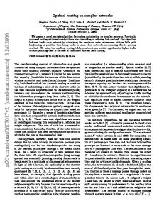
Fig. 1. The bottom plane shows the complete network in which the Overlay nodes are colored. The top plane visualizes the overlay network, in which a tunnel corresponds to an existing, possibly randomized underlay path. The ingress links 1, 2, 3, 4 inject traffic from overlay nodes into the underlay nodes.

I. I NTRODUCTION Overlay networks are a novel concept to bridge the gap between what modern Internet-based services need and what the existing networks actually provide, and hence overcome the shortcomings of the Internet architecture [1], [2]. The overlay creates a virtual network over the existing underlay, utilizes the functional primitives of the underlay, and supports the requirements of modern Internet-based services which the underlay is not able to do on its own (see Fig. 1). The overlay approach enables new services at incremental deployment cost. The focus of this paper is on developing efficient overlay routing algorithms for data which is generated in real-time, e.g., Internet-based applications such as banking, gaming, shopping, or live streaming. Such applications are sensitive to the end-to-end delays experienced by the data packets. Dynamic routing policies for multihop networks have been traditionally studied in the context where all nodes are controllable [3], [4]. Our setup, however, allows only a subset of the network nodes (overlay) to make dynamic routing decisions, while the nodes of the legacy network (underlay) implement simple policies such as FIFO combined with fixed path routing. This approach introduces new challenges because the overlay nodes do not have knowledge of the underlay’s topology, routing scheme or link capacities. Thus, the overlay nodes have to learn the optimal routing policy in an online fashion which involves an exploration-exploitation trade-off between finding low delay paths and utilizing them. Moreover, since the network conditions and traffic demands may be timevarying, this also involves consistently “tracking” the optimal policy.

A. Previous Works The use of overlay architecture was originally proposed in [5] to achieve network resilience by finding new paths in the event of outages in the underlay. In a related work [6] considered the problem of placing the underlay nodes in an optimal fashion in order to attain the maximum “path diversity”. In [7] the authors consider optimal overlay node placement to maximize throughput, while [8] develops throughput optimal overlay routing in a restricted setting. While many works [9], [10] use end-to-end feedbacks for delay optimal routing, these works ignore the queueing aspect, and hence the delay of a packet is assumed to be independent of the congestion in the underlay network. Early works on delay minimization [11], [12] concentrated on quasi-static routing, and do not take the network state into account while making routing decisions. The existing results on dynamic routing explicitly assume that all the network nodes are controllable, and typically analyze the performance of algorithms when the network is heavily loaded [4]. However, in the heavy traffic regime, the delays incurred under any policy are necessarily large, and thus not suitable for routing of realtime traffic. Finally, we note that the popular backpressure algorithm is known to perform poorly with respect to average delays [13]. B. Contributions In contrast to the approaches mentioned above, we consider a network where only a subset of nodes (overlay) are controllable, and propose algorithms that meet average end-to-end

Flow 𝟏 routing links

Link-Level Avg. Queue Bound 𝑩ℓ (𝒕) Tuner Evolutionary Algo.

Flow 𝟐 routing links

𝑺𝒐𝒖𝒓𝒄𝒆𝟏

Underlay Network

1

Replicator Dynamics 𝑩ℓ 𝒕

𝝀ℓ 𝒕

𝑼 𝒕

Packet Level Router 𝑼(𝒕) Q-learning

3

𝑫𝒆𝒔𝒕𝟏

7 8

𝑺𝒐𝒖𝒓𝒄𝒆𝟐 2

Link Price 𝝀ℓ (𝒕) controller Gradient Descent

𝝀ℓ 𝒕

6

5

Primal Dual Algorithm

Fig. 2. The proposed 3 layer Price-based Overlay Controller (POC) comprising of (from bottom to top) i) Overlay nodes making packet-level routing decisions U (t), ii) link-level price controller which manipulates the prices λ` (t), iii) Link-level average queue threshold manipulator which tunes the B` (t). The interactions between the top 2 layers are described by a nonlinear ode called replicator dynamics, while the bottom 2 layers constitute a primaldual algorithm.

delay requirements imposed by applications. Our algorithms are decentralized and perform optimally irrespective of the network load. It follows from Little’s law [14] that for a stable network, the objective of meeting an average end-to-end delay requirement can be replaced by keeping the average queue lengths below some value B. In this work, the problem of maintaining the average queue lengths below B is divided into two subproblems: i) distributing the bound B into link-level average queue thresholds B` such that these link-level bounds can be satisfied under some policy, ii) designing an overlay routing policy that meets the link-level queue bounds imposed by i). We obtain an efficient decentralized solution to ii) by introducing the notion of “link prices” that are charged by links. The link prices induce cooperation amongst the overlay nodes, thereby producing decentralized optimal routing policy, and are in spirit with the Kelly decomposition method for network utility maximization [15]. The average queue lengths are adaptively controlled [16], [17] by manipulating the link prices, but unlike previous works which utilize Kelly decomposition in a static deterministic setting [18], we perform a stochastic dynamic optimization with respect to the routing decisions. In order to solve i) we provide an adaptive scheme which follows the replicator dynamics [19]. Finally, the solutions to i) and ii) are combined to yield a 3 layered queue control overlay routing scheme, see Fig. 2. Our problem also has close connections to the restless Multi Armed Bandit problem (MABP) [20], [21]. Our scheme takes an “explore-exploit strategy” in absence of knowledge regarding the underlay network’s characteristics, and learns the optimal routing policy in an online fashion using the data obtained from network operation. The routing decisions on

9 4

𝑫𝒆𝒔𝒕𝟐

Fig. 3. An overlay network comprising of 2 source destination pairs (1, 3) and (2, 4). Since the routes taken by packets sent at ingress links (1, 5) and (2, 8) share common underlay links (7, 9) and (7, 6), an increase in traffic intensity sent on either of the ingress links may also increase the delay suffered by packets sent on the other ingress link.

the various ingress links (see Fig 3) correspond to the bandit “arms”, while the average end-to-end network delays are the unknown rewards. Since the packets injected by different ingress links share common underlay links on their path, routing decisions at an ingress link ` affect the delays incurred by packets sent on different ingress link `ˆ (see Fig. 3). This introduces dependencies amongst the Bandit arms, and hence the decision space grows exponentially with the number of ingress overlay links. Consequently we cannot apply existing MABP algorithms, and must develop simpler algorithms that suit our needs. Our goal is to develop decentralized policies to control the end-to-end delays, which can be computed efficiently in a parallel and distributed fashion [22]. We show that if the underlay implements a simple static policy, then there exists a decentralized policy that is optimal. When the underlay is allowed to use dynamic policies, we provide theoretical guarantees for our decentralized policies. We begin in Section II by describing the set-up, and pose the problem of designing an overlay policy to keep the average end-to-end delays within a pre-specified bound, as a constrained Markov Decision Process (CMDP) [23]. Section III-A1 solves the problem of meeting link-level average queue bounds. It is shown that the routing decisions across the flows can be decoupled if the links are allowed to charge prices for their usage. This flow-level decomposition technique significantly simplifies the policy design procedure, and also ensures that the resulting scheme is decentralized. Section IV employs an evolutionary algorithm to tune the link-level average queue bounds, and proves the convergence properties. Section VI discusses several useful extensions. Section ?? compares the performance of our proposed algorithms with the existing algorithms. II. P ROBLEM F ORMULATION We will first describe the system model, and then proceed to pose the problem of bounding the average end-to-end delays. A. System Model The network is represented as a graph G = (V, E), where V is the set of nodes, and E is the set of links. The network evolves over discrete time-slots. A link ` = (i, j) ∈ E with

capacity Cl (t), t = 1, 2, . . . implies that node i can transmit Cl packets to node j at time t. We allow for the link capacities C` (t) to be stochastic, i.e., C` (t) depends on the state of link ` at time t. We will assume that the link states are i.i.d. across time 1 . Multiple flows f = 1, 2, . . . , F share the network. Each flow f will be associated with a source node sf and destination node df . We will assume that the packet arrivals at each source node sf are i.i.d. across time and flows2 . Mean arrival rate at source node sf will be denoted by Af . The number of arrivals at any source node are uniformly bounded across time and flows. There are two types of nodes in G: i) overlay: Those that can make dynamic routing and scheduling decisions based on the network state, ii) underlay: Those that implement FIFO scheduling combined with randomized routing, on a per flow basis. The subgraph induced by the underlay nodes will be called the underlay network or just underlay. In order to make the exposition simpler and avoid cumbersome notation, we will make some simplifying assumptions3 . Firstly, the overlay will be assumed to be composed entirely of source and destination nodes. Thus the set of overlay nodes is given by, {i ∈ V : i = sf or i = df for some flow f = 1, 2, . . . , F }. Throughout the paper we will only consider the case where the underlay is weakly connected, i.e., there are no multiple alternating segments of overlay-underlay connecting the source-destination pairs. We will assume that there are no links connecting two overlay nodes directly, i.e., the overlay nodes are connected in the overlay network only through underlay tunnels (see Fig. 1). Also, the flows do not share source nodes. Ingress Links : The network links {` = (i, j) : i ∈ Overlay, j ∈ Underlay} will be referred to as the ingress links. These are the outgoing links from overlay nodes that connect with the underlay, and hence these are precisely the links where the overlay routing decision take place (see Fig. 1). Tunnel: For each outgoing ingress link ` from sf , and a destination node i belonging to overlay, we say that the tunnel τ`,i connects the node sf to i in the overlay network, see Fig. 1. We note that the actual path taken by a packet sent on an ingress link, which is a sequence of underlay links, depends on the randomized routing decision taken by the underlay, and is not known at the overlay. Underlay Operation : The network evolves over discrete time slots indexed t = 0, 1, . . .. Each underlay link ` maintains a separate queueing buffer for each flow in which it stores packets belonging to that flow (see Fig. 4). An underlay link ` is shared by queues belonging to flows whose routes utilize link `. In order to simplify the exposition of ideas, we begin 1 Our analysis extends in a straightforward manner for the case when the states evolve as a finite state Markov process. 2 Our analysis can easily be extended for the case when arrivals are governed by a finite state Markov process. 3 Our algorithms, and their analysis can be easily extended to the case where these assumptions are not satisfied. We choose to present the simple case in order to simplify the exposition of ideas, and avoid unnecessary notation.

Q'(',#)

𝑺𝒐𝒖𝒓𝒄𝒆𝟏

Q'(#,%)

Q)(#,%)

1 𝑫𝒆𝒔𝒕𝟏 Q)(),#)

𝑺𝒐𝒖𝒓𝒄𝒆𝟐

3

𝐐(𝟑,𝟒) = (Q'#,% , Q)(#,%) )

4 𝑫𝒆𝒔𝒕𝟐

2

Fig. 4. An overlay network comprising of 2 flows that share the same destination node 4. Each link ` maintains separate queues for the flows f that are routed on it. Queues on link (3, 4) are given by the vector  Q(3,4) = Q1(3,4) , Q2(3,4) .

by assuming that each underlay link ` implements a static scheduling policy by sharing the available capacity at any time t amongst the flows in some pre-decided ratio. Thus, there arePconstants µ`,f , f = 1, 2, . . . , F ` ∈ E satisfying µ`,f ≥ 0, f µ`,f = 1. At each time t, flow f receives a proportion µ`,f of the available link capacity at link `. Note that in case a flow f does not use the link ` for routing, then µ`,f = 0. The links can use randomization in order to allocate the capacity in the ratio µ`,f . The underlay employs a randomized routing discipline. Thus, once a flow f packet is successfully transmitted on ˆ an underlay link `, P it is routed with a probability P f (`, `) f ˆ Note that ˆ P (`, `) ˆ = 1 ∀f, `, and the routing to link `. ` probabilities are allowed to be flow-dependent. We denote by Rf , the set of links ` which are used for routing flow f packets. Note that this includes static routing such as shortest path. Our analysis extends easily to include the case where the underlay can utilize dynamic routing-scheduling disciplines such as longest queue first, priority based scheduling, or even the Backpressure policy [3]. We discuss the extension in Section VI. Information available to the Overlay: Overlay nodes do not know the underlay’s topology, probability laws governing the random link capacities, nor the policy implemented by it. In Sections III-A1, and IV we will assume that each source node sf knows the underlay queue lengths corresponding to its flow. Later, we will relax this assumption and assume that source nodes know only the end-to-end delays corresponding to its flows. Actions available to the Overlay: Let Q(t) := (Q1 (t), Q2 (t), . . . , QL (t)), where each Q` (t) is a vector containing queue lengths Qf` (t) of all the flows f that are routed through link ` (see Fig. 4). At each time t ≥ 0, each overlay source node sf decides its action U f (t) := {U`f (t)}`=(sf ,i) ,where U`f (t) is the number of flow f packets sent to the queueing buffer of the ingress link ` at time t. This decision is made based on the information available to it until time t which includes f {U f (s), Qf (s), λ(s)}t−1 s=0 , where Q (t) is the vector of queue lengths corresponding to the flow f , and λ(s) = {λ` (s)}`∈E is the vector comprising of link prices at time s.

Scheduling Policy: We will denote vectors in boldface. A routing policy π is a map from Q(t), the vector of queue lengths at time t, to a scheduling action U (t) = {U f (t)}f =1,2,...,F at time t. The action U f (t) determines the number of packets to be routed at time t on each of the ingress links belonging to flow f . Policy at Underlay Throughout, we will assume that the underlay links implement a simple static policy in which each link ` shares the link capacity C` amongst the flows in some constant ratio, even if some of the queues Qf` (t) are empty. In Section VI we will provide guidelines to consider the case when such an assumption is not true, i.e., the underlay network implements a more complex policy. B. Objective: Keep Average Delays Bounded by B We now pose the problem of designing an overlay routing policy that meets a specified requirement on the average endto-end delays incurred by packets as a constrained MDP [23]. For a stable network, it follows from the Little’s law [14], that for a fixed value of the mean arrival rate, the mean delay is proportional to the average queue lengths. Thus, we will focus on controlling the average queue lengths instead of bounding the end-to-end delays. A bound on the average queue lengths will imply a bound on the average end-to-end delays. Since now our objective is to control the average queue lengths, the state ( [24]) of the network at P time t is specified by the vector Q(t). Also, we let kQ(t)k := `,f Qf` (t) denote the total queue length, i.e. the 1 norm of the vector Q(t). We also let Qf (t) := {Qf` (t)}`∈Rf denote the vector containing queue lengths belonging to flow f . The queue dynamics are given by,  + Qf` (t + 1) = Qf` (t) − D`f (t) + Af` (t), ∀f, `, where D`f (t), Af` (t) are the number of flow f departures and arrivals respectively at link ` at time t. The arrivals could be external, or due to routing after service completions at other links. If the overlay knew the underlay topology, link capacities and routing policy, the overlay could solve the following constrained MDP [23] in order to keep the average queue lengths less than the threshold B,

{U f (t)}f =1,2,...,F , the overlay routing decision at time t is solely determined by the network state, i.e., U (t) = h(Q(t)). The assumption of bounded queues is not overly restrictive since the links can simply drop a packet if their buffer overflows4 . We note that we can also consider the set-up in which each flow f has an average end-to-end delay requirement, and the objective is to design an overlay routing policy that meets the requirements imposed by each flow f . We exclude this set-up to make the presentation easier, and instead focus only on the case where the delays summed up over flows is to be kept below a certain threshold. Details regarding this extension can be found in Section VI. ¯ Henceforth we will write kQk π to denote the total steady state average queue lengths under the application of policy π. ¯ instead We will suppress the dependency on π and use kQk ¯ . Similarly for kQ¯` k, Q ¯ f etc. of kQk π ` III. O PTIMAL P OLICY D ESIGN We now begin our analysis when the underlay implements a static policy. We will show that it is possible to construct an optimal decentralized overlay routing policy using a 3 layered controller as shown in Figure 2. The topmost layer will manipulate “link-level average queue thresholds” B` (t) based on the link prices λ` (t). The link prices λ` (t) are representative of the instantaneous congestion at link `. The next two layers, link-price controller, and packet-level decision maker will collectively try to meet the bounds B` (t) by using a primal dual algorithm described below. The packet-level decision maker will utilize the link prices λ` (t) in order to make routing decisions U (t). It will transmit packets on routes which utilize links with lower prices. The link-price controller will then observe the congestion that results from the routing decisions U (t), and manipulate the prices accordingly in order to direct more traffic towards links on which the average queues are less than the threshold B` (t). The interaction between the top two layers is described by a nonlinear ordinary differential equation (ode) called the replicator equation [19]. Fig. 2 depicts the interactions between these layers. We call our 3 layered adaptive routing policy Price-based Overlay Controller (POC). We now develop these algorithms in a bottom to top fashion. A. Link-level Design

min 0

(1)

π

1 Eπ T →∞ T lim

(

T X

) kQ(t)k

≤ B,

(2)

t=1

where expectation is taking with respect to the (possibly random) routing policies at the overlay and underlay, and the randomness of arrivals and link capacities. If we assume that the network queue lengths are uniformly bounded, i.e., Qf` (t) ≤ C, ∀` ∈ E, f = 1, 2, . . . , F , then standard theory from constrained MDP [23] tells us that the above is solved by a stationary randomized policy. Thus U (t) =

P ¯ We notice that in order to satisfy the constraint ` kQ `k ≤ B imposed in the CMDP (1), a policy π needs to appropriately coordinate the individual link-level average queue lengths ¯ ` k in order that their combined value is less than B. kQ Such a task is difficult because the link-level average queues ¯ ` k have complex interdependencies between them that are kQ described by the unknown underlay network structure. 4 The steady state packet loss probabilities can be made arbitrarily small by choosing the bound C to be sufficiently large. Moreover, such an assumption automatically guarantees stability of queues, and lets us focus on our key objective of controlling network delays.

Tunes Link Level Avg. Queue Bounds 𝐁(𝒕) 𝝀𝟏 (𝒕) 𝝀𝟒 (𝒕)

𝝀𝟏 (𝒕)

𝑨𝒓𝒓𝟏

1

𝝀𝟏 (𝒕)

5

𝝀𝟑 (𝒕)

𝝀𝟐 (𝒕) 𝝀𝟒 (𝒕)

𝝀𝟐 (𝒕)

𝑨𝒓𝒓𝟐

𝝀𝟑 (𝒕)

𝝀𝟐 (𝒕)

8

2

𝝀𝟑 (𝒕)

𝟏

3

𝑫𝒆𝒔𝒕𝟏

4

𝑫𝒆𝒔𝒕𝟐

𝟒 𝟐 𝟑

𝝀𝟒 (𝒕)

Fig. 5. An overlay network comprising of 2 source destination pairs (1, 3) and (2, 4). The introduction of link prices λ` (t) decouples the routing decisions at the overlay and results in a decentralized scheme. It also serves as a mediator between the overlay nodes making routing decisions, and the tuner which sets the queue thresholds B` .

thresholds B` neatly decomposes into F sub-problems, one for each flow. The sub-problem for flow f is to route Pits packets ¯f . in order to minimize its individual holding cost ` λ` Q ` We now proceed to solve the CMDP (3). Throughout this section we will assume that (3) is feasible, i.e., there exists a routing policy π under which the average queue lengths are less than or equal to the thresholds B` . Let λ` ≥ 0 denote the Lagrange multiplier associated with the constraint kQ¯` k ≤ B` , and let λ = (λ1 , λ2 , . . . , λL ). If π is a stationary randomized policy ( [23], [25]), then the Lagrangian for the problem (3) is given by [23], X
L(π, λ) = λ` kQ¯` k − B` `

=

X

  X f X ¯ − λ`  Q λ` B` `

`

f

`

 In view of the above discussion, we begin by considering a simpler problem, one in which the tolerable cumulative average queue bound B has already beenPdivided into linklevel “components” {B` }`∈E that satisfy `∈E B` = B, and the task of overlay is to keep the average queues on each link ` bounded by the quantity B` . An efficient scheme should be able to meet the link-level bounds B` in case they are achievable under some routing scheme. Thus, we consider the following Constrained MDP [23], min π

0

s.t. kQ¯` k ≤ B` ,

(3) ∀` ∈ E,

(4)

where in the above, expectation is taken with respect to the overlay policy π, randomness of packet arrivals, network link capacities and the underlay policy. Next, we derive an iterative scheme that yields a decentralized policy which solves the above CMDP, i.e., satisfies the link-level average queue length bounds in case they are achievable under some policy. The task of choosing the bounds B` will be deferred until Section IV. 1) Flow Level Policy Decomposition: We now show that the problem (3) of routing packets under average delay constraints at each link ` ∈ E admits a decentralized solution of the following form. Each underlay network link ` charges a “holding cost” at the rate of λ` units per unit queue length Qf` from each flow f that utilizes link `. The holding charge collected by link ` from flow f at time t is thus λ` (t)Qf` (t). The flows are provided with the link prices {λ` }`∈E , and they schedule their packet transmissions in order to minimize their P ¯f average holding costs ` λ` Q` . Under such a scheme, the prices λ` intend to keep the network traffic from “flooding” the links, thus enabling them to meet the average queue threshold of B` units. The routing scheme described above is decentralized, meaning that each flow f makes the routing decisions solely based on its individual queue lengths Qf (t), and the link prices λ, and not on the basis of global state vector Q(t). Thus, the problem of routing packets in order to meet the average queue

=

 X

X 

¯f  − λ` Q `

X

`∈Rf

f

λ` B` ,

(5)

`

where the second equality follows from the relation kQ` (t)k = P f f Q` (t). The Lagrangian thus decomposes into the sum of P ¯ f , where Rf is the set of flow f “holding costs” `∈Rf λ` Q ` links utilized for routing packets of flow f . We now make the following important observation. Since the links share the service amongst its queues in a manner irrespective of the queue length Q` (t), the service received by flow f on link ` at any time t, is determined only by the capacity of link ` at time t, and queue length Qf` (t). Thus, the evolution of queue length process Qf (t), t ≥ 0 is completely described by U f (t), t ≥ 0, i.e., the routing actions chosen for flow f at source node sf , and the probability laws governing capacities of links ` that are used to route flow f packets. Let us denote by πf a policy for flow f that maps Qf (t) to U f (t). P ¯ f incurred Since for a fixed value of λ, the cost `∈Rf λ` Q ` by each flow f can be optimized independently of the policies chosen for other flows, it then follows from (5) that, Lemma 1: The dual function corresponding to the CMDP (3) is given by, D(λ) = min L(π, λ) π X X X ¯f − = min λ` Q λ` B` ., ` f

πf

`∈Rf

(6)

`

and hence the policy π which minimizes the Lagrangian for a fixed value of λ is decentralized. We now provide a precise definition of a decentralized policy. Decentralized Policy: A policy π is said to be decentralized if U f (t), i.e., the overlay decisions regarding packets of flow f , are made based solely on the knowledge of flow f queues Qf (t), i.e., U f (t) = hf (Qf (t)). If π is decentralized, we let π = ⊗f πf , i.e., π is uniquely identified by describing the policies πf for each individual flow f . Upon associating a policy with the steady state measure that it induces on the joint state-action pairs, we see that the decentralized policy corresponds to the product measure ⊗f πf on the space

⊗f (Qf , Uf ), where Qf is the space on which Qf (t) resides, and Uf is the action space corresponding to the routing decisions for flow f . Let λ? be the value of the Lagrange multiplier that solves the dual problem, i.e., λ? ∈ arg max D(λ), λ≥0

(7)

where 0 is the |E| dimensional vector all of whose entries are 0. The average costs incurred under a policy π can be considered as a dot product between the steady state probabilities induced over the joint state-action pair under π, and the one-step cost under state-action pairs. Hence, a CMDP can equivalently be posed as a linear program [26], and is convex. Thus, the duality gap corresponding to the problem (3), and its dual (7) is zero [27]. Let us denote by πf? (λ) the policy for P ¯f . flow f which minimizes the holding cost `∈Rf λ` Q ` It then follows from the above discussion that, Theorem 1: There exists λ? = {λ?` } ≥ 0 such that the CMDP (3) is solved by the policy π ? which implements for each flow f the corresponding policy πf? (λ? ). Thus, π ? = ⊗f πf? (λ? ), i.e., the optimal policy for the CMDP (3) is decentralized. The consideration of the dual problem corresponding to CMDP (3) greatly reduces the problem complexity. We were able to show that the optimal policy is decentralized. As will be discussed in Section VIII-B, this has several advantages. However, the following two issues need to be addressed in order to compute the optimal policy π ? . 1) Computation of the policies πf? (λ) requires the knowledge of underlay topology, distribution of underlay links’ capacities and statistics of packet arrival processes. These are, however, not known at overlay. Moreover, in case the parameters are time-varying, the policy πf? (λ) necessarily needs to adapt to the changes. 2) Optimal policy π ? in Theorem 1 needs to know the vector of optimal “link prices” λ? that solve the dual problem (7). Next, we resolve these issues. IV. A DAPTIVELY T UNING AVERAGE Q UEUE BOUNDS B` The scheme (23)-(24) developed in Section III-A1 keeps the average delays bounded by thresholds {B` }`∈E that have been provided by the network operator. However, it works only if the thresholds {B` }`∈E are achievable. Thus, while developing the scheme we had implicitly assumed that the overlay knew that the link-level average queue threshold profile {B` }`∈E could be met, and thereafter it could utilize the Algorithm of Theorem 4 in order to meet the delay requirements. But, the assumption that the overlay is able to characterize the set of achievable thresholds {B` }`∈E is hard to justify in practice. Characterization of the set of achievable {B` }`∈E is difficult because of the complex dependencies between various link-level delays. Furthermore, in order to calculate

the average delay performance for any fixed policy π, the overlay needs to know the underlay characteristics, which we assume are unknown to the overlay. Thus, in this section, we devise an adaptive scheme that measures the link prices λ` that result when the scheme (23)-(24) is applied to the network, and utilizes them to iteratively tune the P delay thresholds B` until an achievable vector B satisfying ` B` = B is obtained. The key feature of the resulting scheme is that it does not require the knowledge of the underlay network characteristics. It increases the bounds B` for links with “higher prices”, and decreases B` for links with “lower prices”, while simultaneously ensuring that the new bounds sum up to B. It is shown in Lemma 9 that the price iterations in (23) ¯ converge for each fixed B. Let us denote by λ(B) := ¯ ` (B)}`∈E the vector comprising of link prices that result {λ when the average queue thresholds are set at B, and the iterations (23)-(24) are performed untill convergence. Thus, ¯ λ(B) denotes the steady-state link prices when the scheme of Theorem 4 is utilized with thresholds set to B. We propose the following iterative scheme to tune the delay budget vector B(t), B` (k + 1) ( = Γ B` (k) + γk

¯ B` (k) λ(B(k)) −

X

!)! ¯ λ` (B(k))B` (k) ,

`

(8) ∀` ∈ E, where k is the iteration index, and Γ (·) is the projection operator that maps the vector B(k) ∈ RL onto the L dimensional simplex ( ) L X S= x: xi = B, xi ≥ 0 ∀i = 1, 2, . . . , L . i=1

Projection P operator Γ (·) is required in order that the iterates satisfy ` B` = B. We will show that the iterations (8) converge to anPachievable vector B under which the total delay threshold ` B` is less than B. We will utilize the ODE method ( [28]–[30]) in order to analyze the discrete recursions (8). We will build some machinery in order to be able to utilize the ODE method. In a nutshell, the ODE method says that the discrete recursions (8) asymptotically track the ode, ! X ¯ ` (B(t)) − ¯ ` (B(t))B` (t) , ∀` ∈ E. B˙ ` = B` (t) λ λ `

(9) A more precise statement is as follows. ˜ Lemma 2: Define a continuous time process B(t), t ≥ 0, t ∈ R in the following manner. Define time instants s(n), n = Pn−1 0, 1, . . . by setting s(n) = m=0 γm . Now let ˜ B(s(n)) = B(n), n = 0, 1, 2, . . . .

Then use linear interpolation on each interval [s(n), s(n + 1)] ˜ to obtain values of B(t) for the time interval [s(n), s(n + 1)]. Then for any T > 0, lim

sup

s→∞ t∈[s,s+T ]

˜ − B s (t)k2 = 0, kB(t)

(10)

where B s (t), t ≥ s is a solution of (9) on [s, ∞) with B s (t) = ˜ B(s). Thus, the recursions can be viewed as discrete analogue of the corresponding deterministic ode. Proof: A detailed proof of (10) can be found in [28] Ch:5 Theorem 2.1. We note that the discrete-time process B(k), k = 0, 1, . . . of (8) is deterministic. However, the recursions (8) do assume ¯ that the price vector λ(B(k)) is available in order to carry out the update. It now follows from Lemma 2 that in order to study the convergence properties of the recursions (8), it suffices to analyze the detrministic ode (9). We identify the above ode as the replicator equation [19], which has been utilized in evolutionary game theory. Next, we will make some assumptions regarding the replicator ode (9), and show that the trajectory of the ode has the desired properties under these assumptions. Let h·, ·i denote the dot product of two vectors. Definition 1: The ode (9) satisfies the monotonicity condition [31] if D E ¯ ¯ B) ˆ λ(B) ˆ < 0, ∀B 6= B ˆ ∈ S. B − B, − λ( (11) We have, Lemma 3: If the ode (9) satisfies the monotonicity condition, then for B(0) in the interior of S, B(t), the solution of the ode (9) satisfies B(t) → B ? , which is the unique equilibrium point of (9). Lemmas 2 and 3 guarantee that the algorithm that starts with a suitable value of the delay budget vector B(0), and then tunes it according to the rule (8) converges to a feasible value of the delay budget vector B ? . Once the feasible B ? has been obtained, the scheme (23) can be used in order to route packets. In summary, Theorem 2: [Replicator Dynamics based B tuner] For the iterations (8), we have that B(k) → B ? , and hence the average queue lengths under the scheme described above are bounded by B. Proof: It follows from Lemma 2 that the recusions (8) asymptotically track the ode (9) in the “γ → 0, k → ∞” limit (see Ch: 5 of [28], or Ch: 2 of [30]). Since the trajectory B(t) of the corresponding ode (9) satisfies B(t) → B ? , the proof follows. Remark 1: It must be noted that whether or not the delay bound B is achievable depends upon the network characteristics and traffic arrivals. Hence, if the bound B is too ambitious, it may not be achievable. In this case, the condition (11) will clearly not hold true, and the evolutionary algorithm will not be able to allocate the delay budgets appropriately. Thus, it is required that the network operator calculate an estimate of the value of the bound B that can be achieved, using knowledge

of the arrival processes, underlay link capacities etc. Another way to choose an appropriate value of B can be to simulate the system performance under a “reasonably good policy”, and set B equal to the average delays incurred under this policy. Remark 2: We note the important role that the link-prices λ` play in order to “signal” to the tuner about the underlay network’s characteristics. Thus, for example, a link ` might be strategically located, so that a large chunk of the network traffic necessarily needs to be routed through it, thus leading to a large value of average queue lengths under any routing policy π. Alternatively, its reliability might be low, which again leads to large value of queue lengths Q` (t). In either case, the quantity B`? would converge to a “reasonably large value”, which in turn is enabled by high values of prices λ` during the course of iterations (8). A. Tuning B using online learning The scheme proposed in Theorem 2 needs to compute the ¯ prices λ(B(k)) in order to carry out the k-th update. One ¯ way to compute the λ(B(k)) is to apply Algorithm (23) with thresholds set to B(k), and wait for the link prices to ¯ converge to λ(B(k)). In order to speed up this naive scheme, we would like to carry out the B` updates in parallel with the iterations (23)-(24), an idea that is similar to the two timescale stochastic approximation scheme of Section VIII-A3. Thus, we propose the following scheme that comprises of three iterative update processes evolving simultaneously,  V (Qf (t), U f (t)) ← V (Qf (t), U f (t)) (1 − αt )   X  + αt λ` Qf` (t) + min V (Qf (t + 1), uf ) − V (q0 , u0 ) ,   uf `∈Rf

(12) λ` (t + 1) = M {λ` (t) + βt (kQ` (t)k − B` )} , ∀` ∈ E, (13) B` (t + 1) ( = Γ B` (t) + γt

!)! B` (t) λ` (t) −

X

λ` (t)B` (t)

,

`

(14) ∀` ∈ E, where the step sizes satisfy βt = o(αt ), γt = o(βt ). The condition γt = o(βt ) will ensure that the B recursions view the network-wide link prices as having equilibriated for a fixed value of B. Next, we show that such a scheme, depicted in Algorithm 1, in which the B updates occur in parallel with the price cum Q-learning iterations, does indeed converge. The analysis is similar to the two time-scale stochastic approximation scheme discussed in the previous section. Its proof is provided in Appendix. Theorem 3: [Three Time-scale POC Algorithm] For the iterations (8), almost surely, B(t) → B ? . Hence, the average

Algorithm 1 Price-based Overlay Controller (POC) centralized optimal controller that has been obtained by P 2 P solving the constrained MDP (1) using Linear Prgoramming Fix P sequences αP , β , γ satisfying α < ∞, α = t t t t t P P ∞, βt2 < ∞, βt = ∞, γt2 < ∞, γt = ∞, and approach. Firstly, the link prices λ` play the role of coordinating the actions of different flows. This allows us to βt = o(αt ), γt = o(βt ). P reduce the problem of jointly scheduling F flows (1), to much Initialize λ(0) > 0, B(0) such that ` B` (0) = B. simpler sub-problems that involve designing policy for only a Perform the following iterations. single flow. As discussed earlier, the computational complexity 1) Each source node sf updates its Q-values using, scaled linearly with the number of flows, as compared with  V (Qf (t), U f (t)) ← V (Qf (t), U f (t)) (1 − αt ) exponential in F . ( ) X The algorithms proposed until now assume that the overlay + αt λ` Qf` (t) + min V (Qf (t + 1), uf ) − V (q0 , u0 ) source , nodes sf know which underlay links route its packets. `

uf

If these are unknown, then we can utilize Algorithm 1 on the overlay network comprising of tunnels. Thus, each overlay ˆ fτ (t) for each and the routing action implemented for flow f at time t source node sf maintains “virtual queues” Q f is arg maxuf ∈Uf V (Q (t), uf ). of its outgoing tunnel τ . Since link-level queue lengths are ˆ fτ (t) are set to be equal to the “number of packets 2) Overlay updates the link prices according to, unknown, Q in flight” on tunnel τ , i.e., the number of packets that have λ` (t + 1) = M {λ` (t) + βt (kQ` (t)k − B` )} , ∀` ∈ E. been sent on tunnel τ , but have not reached their destination (16) node by time t. The link prices and link-level average queue 3) Overlay adapts the link-level delay requirements accord- threshold requirements are now replaced by their tunnel couning to, terparts λτ (t), Bτ (t). Their iterations proceed in exactly the same manner as in Algorithm 1. The routing algorithm is much B` (t + 1) ( !)! simpler, so that each source routes packets on its tunnel with X the least price λτ (t). This yields the tunnel level POC, which is = Γ B` (t) + γt B` (t) λ` (t) − λ` (t)B` (t) , denoted POC-T (tunnel level POC) described in Algorithm 2. (15)

`

(17) ∀` ∈ E.

queue lengths suffered under the Price-based Overlay Controller (POC) described in Algorithm 1 are bounded by B. V. P UTTING IT ALL TOGETHER : T HREE L AYER POC Algorithm 1 is composed of the following three layers from top to bottom: 1) Replicator Dynamics based B` tuner that observes the link prices λ` , and increases/decreases B` appropriately while keeping their sum equal to B. 2) Sub-gradient descent based λ` tuner that is provided the delay budget B` by the layer 1 described above, observes the queue lengths Q` and updates the prices based on the ¯`. mismatch between B` and Q 3) Q-learning based routing policy learner which is provided the link prices λ` , and learns to minimize the holding cost ¯ f . Its actions reflect the congestions on various links λ` Q ` ¯ f , which in turn are used by layer through the outcomes Q ` 2 above. The above three layers are thus intimately connected and coordinate amongst themselves in order to attain the goal of keeping the average queue lengths bounded by B. This is shown in Figure 2. VI. C OMPLEXITY OF POC AND POSSIBLE E XTENSIONS We discuss about the enormous simplification and reduced computational complexity of the POC as compared to the

Algorithm 2 Tunnel Level POC (POC-T) Fix sequences αt , βt , γt satisfying conditions of Algorithm 1. P Initialize λ(0) > 0, B(0) such that τ Bτ (0) = B. Perform the following operations. 1) Each source node sf updates the tunnel queues, ˆ fτ (t) = Q ˆ fτ (t − 1) + Afτ (t) − Dτf (t), Q where Afτ (t) are the number of flow f packets that are routed to tunnel τ at time t, and Dτf (t) are the number of flow f packets that had been routed through tunnel τ , and reach their destination node at time t. The node sf routes packets to the tunnel τ with the least holding cost ˆ f (t). λτ (t)Q τ 2) Tunnel prices are updated as, n  o ˆ τ (t) − Bτ λτ (t + 1) = M λτ (t) + βt Q . 3) The tunnel-level average queue thresholds Bτ are updated according to, Bτ (t + 1) ( = Γ Bτ (t) + γt

Bτ (t) λτ (t) −

!)! X

λτ (t)Bτ (t)

τ

Another important generalization is to consider the case ¯f k where each flow f requires its average queue lengths kQ to be bounded by a threshold. The POC Algorithm can bemodified so that it now maintains B`f , i.e., link-level queue

.

bounds for each flow f . Similarly, links maintain λf` , i.e., separate prices for each flow f and the routing for P algorithm ¯f . flow f seeks to minimize the holding cost `∈Rf λf` Q ` We can also consider the case where underlay implements a dynamic policy such as largest queue first, or backpressure policy [32]. The convergence of our proposed algorithms to the optimal policy, i.e., Theorems 4, 3 will continue to hold true in this set-up. Denote by πul the policy being implemented at the underlay. The proof of Theorem 4 will then be modified by using the fact that for a fixed value of price vector λ, the steady-state control policy applied to the network is given by (π ? (λ), πul ). Since the resulting controlled network still evolves on a finite state-space, and the policy (π ? (λ), πul ) is stationary, it is easily verified that the conclusions of Lemmas 6-8, Theorem 4, and the results of Section IV-A hold true. Yet another possibility is to consider the case where the data packets have hard deadline constraints, i.e., they should reach their destination within a prespecified deadline in order for them to be counted towards “timely-throughput”. Real-time traffic usually makes such stringent requirements on meeting end-to-end deadlines. A metric to judge the performance of scheduling policies for such traffic is the timely-throughput metric [33]. Timely throughput of a flow is the average number of packets per unit time-slot that reach their destination node within their deadline. The POC algorithm can be modified in order to maximize the cumulative timely-throughput of all the flows in the network. The packet-level router would then maximize the timely throughput minus the cost associated with using link bandwidth, which is priced at λ` units. Moreover, the topmost Replicator Dynamics based layer will not be required, and will be removed. The pricing updates will now be modified, so that they will try to meet the link capacities C` , and not the average queue delays at link `. A detailed treatment for the case when the network is controllable can be found in [34]. In this paper we have allowed for control at only the source nodes. In practice, it may be desirable to control some intermediate nodes, since that would enable us to attain a lower value of average queue lengths. A modification to the bottommost layer will enable POC to handle such situations. Thus, each controllable node i will have to perform Q-learning updates (12) in order to “learn” its optimal routing policy. Thereafter, at each time t, it will make routing choices based on the instantaneous queue lengths Qf (t), and the link prices λ by utilizing the optimal routing policy generated via Qlearning. VII. C ONCLUSIONS We have analyzed optimal overlay routing problem in the system where the network operator has to satisfy a performance bound of average end-to-end delays less than D units. The problem is challenging because the overlay does not know the underlay characteristics. We proposed a simple decentralized algorithm based on a 3 layered adaptive control design. The algorithms could easily be tuned to operate under

a vast multitude of information available about the underlay congestion. We also propose a heuristic scheme in case the flows do not know the links that are used to route their traffic. Simulations results show that the proposed schemes significantly outperform the existing policies. R EFERENCES [1] R. K. Sitaraman, M. Kasbekar, W. Lichtenstein, and M. Jain, “Overlay networks: An akamai perspective,” Advanced Content Delivery, Streaming, and Cloud Services, pp. 305–328, 2014. [2] L. L. Peterson and B. S. Davie, Computer networks: a systems approach. Elsevier, 2007. [3] L. Tassiulas and A. Ephremides, “Stability properties of constrained queueing systems and scheduling policies for maximum throughput in multihop radio networks,” IEEE Transactions on Automatic Control, vol. 37, no. 12, pp. 1936–1948, Dec 1992. [4] A. L. Stolyar, “Maxweight scheduling in a generalized switch: State space collapse and workload minimization in heavy traffic,” The Annals of Applied Probability, vol. 14, no. 1, pp. 1–53, 02 2004. [5] D. Andersen, H. Balakrishnan, F. Kaashoek, and R. Morris, Resilient overlay networks. ACM, 2001, vol. 35, no. 5. [6] J. Han, D. Watson, and F. Jahanian, “Topology aware overlay networks,” in Proceedings IEEE 24th Annual Joint Conference of the IEEE Computer and Communications Societies., vol. 4. IEEE, 2005, pp. 2554– 2565. [7] N. M. Jones, G. S. Paschos, B. Shrader, and E. Modiano, “An overlay architecture for throughput optimal multipath routing,” in Proceedings of the 15th ACM international symposium on Mobile ad hoc networking and computing. ACM, 2014, pp. 73–82. [8] G. S. Paschos and E. Modiano, “Throughput optimal routing in overlay networks,” in Communication, Control, and Computing (Allerton), 2014 52nd Annual Allerton Conference on. IEEE, 2014, pp. 401–408. [9] J. A. Boyan and M. L. Littman, “Packet routing in dynamically changing networks: A reinforcement learning approach,” Advances in neural information processing systems, pp. 671–671, 1994. [10] B. Awerbuch and R. D. Kleinberg, “Adaptive routing with end-to-end feedback: Distributed learning and geometric approaches,” in Proceedings of the thirty-sixth annual ACM symposium on Theory of computing. ACM, 2004, pp. 45–53. [11] R. Gallager, “A minimum delay routing algorithm using distributed computation,” IEEE transactions on communications, vol. 25, no. 1, pp. 73–85, 1977. [12] J. Tsitsiklis and D. Bertsekas, “Distributed asynchronous optimal routing in data networks,” IEEE Transactions on Automatic Control, vol. 31, no. 4, pp. 325–332, 1986. [13] L. Bui, R. Srikant, and A. Stolyar, “Novel architectures and algorithms for delay reduction in back-pressure scheduling and routing,” in INFOCOM 2009, IEEE. IEEE, 2009, pp. 2936–2940. [14] S. Asmussen, Applied Probability and Queues. Wiley, 1987. [15] F. P. Kelly, A. K. Maulloo, and D. K. H. Tan, “Rate control for communication networks: Shadow prices, proportional fairness and stability,” The Journal of the Operational Research Society, vol. 49, no. 3, pp. pp. 237–252, 1998. [16] K. J. Astrom and B. Wittenmark, Adaptive Control, ser. Dover Books on Electrical Engineering. Dover Publications, 2008. [17] V. Borkar and P. Varaiya, “Adaptive control of Markov chains, I: Finite parameter set,” IEEE Transactions on Automatic Control, vol. 24, no. 6, pp. 953–957, Dec 1979. [18] D. P. Palomar and M. Chiang, “A tutorial on decomposition methods for network utility maximization,” IEEE Journal on Selected Areas in Communications, vol. 24, no. 8, pp. 1439–1451, 2006. [19] J. Weibull, “Evolutionary game theorymit press,” Cambridge, MA, 1995. [20] J.C. Gittins, K. Glazebrook and R. Weber, Multi-armed Bandit Allocation Indices. John Wiley & Sons, 2011. [21] T. L. Lai and H. Robbins, “Asymptotically efficient adaptive allocation rules,” Advances in applied mathematics, vol. 6, no. 1, pp. 4–22, 1985. [22] D. P. Bertsekas and J. N. Tsitsiklis, Parallel and distributed computation: numerical methods. Prentice hall Englewood Cliffs, NJ, 1989, vol. 23. [23] E. Altman, Constrained Markov Decision Processes. Chapman and Hall/CRC, March 1999. [24] D. Bertsekas, Dynamic Programming and Optimal Control, 2nd ed. Athena Scientific, 2001, vol. 1 and 2.

[25] M. L. Puterman, Markov Decision Processes: Discrete Stochastic Dynamic Programming, 1st ed. New York, NY, USA: John Wiley & Sons, Inc., 1994. [26] V. S.Borkar, “A convex analytic approach to Markov decision processes,” Probability Theory and Related Fields, vol. 78, no. 4, pp. 583– 602, 1988. [27] D. P. Bertsekas, A. E. Ozdaglar, and A. Nedic, Convex analysis and optimization, ser. Athena scientific optimization and computation series. Belmont (Mass.): Athena Scientific, 2003. [28] H. J. Kushner and G. Yin, Stochastic Approximation Algorithms and Applications. New York: Springer Verlag, 1997. [29] V. S. Borkar and S. P. Meyn, “The o.d.e. method for convergence of stochastic approximation and reinforcement learning,” SIAM Journal on Control and Optimization, vol. 38, no. 2, pp. 447–469, 2000. [30] V. S. Borkar, Stochastic Approximation : A Dynamical Systems Viewpoint. Cambridge: Cambridge University Press New Delhi, 2008. [31] H. Smith, Monotone dynamical systems. Providence, RI: American Mathematical Society, 1995. [32] “Technical report,” https://www.dropbox.com/s/v5d5svfpypfdieq/ technical%20report.pdf?dl=0. [33] I-Hong Hou and V.S. Borkar and P.R. Kumar, “A Theory of QoS for Wireless,” in IEEE INFOCOM 2009, April 2009, pp. 486–494. [34] R. Singh and P. Kumar, “Throughput optimal decentralized scheduling of multi-hop networks with end-to-end deadline constraints: Unreliable links,” arXiv preprint arXiv:1606.01608, 2016. [35] J. Abounadi, D. Bertsekas, and V. S. Borkar, “Learning algorithms for markov decision processes with average cost,” SIAM Journal on Control and Optimization, vol. 40, no. 3, pp. 681–698, 2001. [36] R. S. Sutton and A. G. Barto, Reinforcement Learning: An Introduction. MIT Press, 1998. [Online]. Available: http://www.cs.ualberta.ca/\% 7Esutton/book/ebook/the-book.html [37] J. N. Tsitsiklis, “Asynchronous stochastic approximation and qlearning,” Machine Learning, vol. 16, no. 3, pp. 185–202, 1994. [38] T. Jaakkola, M. I. Jordan, and S. P. Singh, “On the convergence of stochastic iterative dynamic programming algorithms,” Neural computation, vol. 6, no. 6, pp. 1185–1201, 1994. [39] H. J. Kushner and D. S. Clark, Stochastic approximation methods for constrained and unconstrained systems. Springer Science & Business Media, 2012, vol. 26. [40] V. R. Konda and J. N. Tsitsiklis, “Actor-critic algorithms.” in NIPS, vol. 13, 1999, pp. 1008–1014. [41] V. S. Borkar, “An actor-critic algorithm for constrained markov decision processes,” Systems & control letters, vol. 54, no. 3, pp. 207–213, 2005. [42] W. F. Ames and B. Pachpatte, Inequalities for differential and integral equations. Academic press, 1997, vol. 197. [43] K. C. Border, Fixed point theorems with applications to economics and game theory. Cambridge university press, 1989.

VIII. A PPENDIX A. Using Multiple Time-scale based Online Learning methods 1) Employing Online Learning to Obtain πf? (λ): We can utilize online learning methods such as Relative Value Iteration (RVI) Q-learning [35] in order to obtain πf? (λ), i.e., the P ¯ f for flow f . policy that minimizes the holding cost ` λ` Q ` Each overlay source node sf maintains the Q-values [35], [36] V (q f , uf ) which corresponds to the “long-term” utility obtained by taking the routing action uf when the flow f queue vector is q f . These Q-values are updated using online data as follows,  V (Qf (t), U f (t)) ← V (Qf (t), U f (t)) (1 − αt )   X  + αt λ` Qf` (t) + min V (Qf (t + 1), uf ) − V (q0 , u0 ) ,   uf `∈Rf

(18) where αt = 1t , and (q0 , u0 ) is a fixed state-action pair. The routing action implemented at time t corresponds to the

action uf that minimizes the quantity V (Qf (t + 1), uf ). Convergence of the Q-learning scheme to the optimal policy is well-understood, and detailed convergence proofs can be found in [28], [30], [37], [38]. We however state this as a lemma since it will be required in convergence analysis of later sections, when we will combine the Q-learning iterations with other iterative algorithms. Lemma 4: The asymptotic properties of the stochastic iterations (18) can be derived by studying the following ordinary differential equation (ode), V˙ = T V − eV (q0 , u0 ),

(19)

where T is the Bellman operator, i.e., T V (q, u) = kqk + ˜ u)}, and e is vector comprising of all ones. E {minu V (q, Since the mapping V 7→ T V − V is contractive, the ode (19), and hence the Q-learning iterations (18) converge, thus yielding the optimal routing policy. Proof: See [35]. We note that the Q-learning algorithm as discussed above learns the optimal policy, i.e., a mapping from the instantaneous queue lengths Qf (t) to a routing action U f (t). It does not require the knowledge of the dynamics of queue lengths evolution in the network, and this is precisely the reason why we employ Q-learning, because the queue dynamics are unknown to the policy at the overlay. 2) Obtaining λ? using Subgradient Descent Method: Next, we address the issue of obtaining the optimal value of vector of link prices λ? . Let us, for the time being, assume that for a given value of link prices λ, the policy π ? (λ) has been obtained. This could be achieved, for example, by performing the Q-learning iterations until convergence. Since, D(λ) = L(π ? (λ), λ),

(20)

and from (5), ∂L = kQ¯` k − B` , ∀` ∈ E, ∂λ` we can use the gradient descent method [27] to compute λ? via the following iterations,
λ` (k + 1) = λ` (k) + βk kQ¯` k − B` , ∀` ∈ E, (21) where kQ¯` k is the steady state average queue lengths at link ` under the application of π ? (λ(k)), while βk can be taken to be k1 . We state the convergence result since it will be utilized later. Lemma 5: The following ode λ˙ = ∇λ D(λ)

(22)

converges to λ? the solution of the dual problem (20), and hence the iterations (21) converge to λ? . Since the price iterations (21) track the ode (22) in the βk → 0, k → ∞, they too converge to optimal price λ? . Proof: In order to analyze the properties of the ode (22), let us take the value of the dual function D. We then have, d D(λ(t)) = −k∇λ D(λ(t))k2 ≤ 0. dt

Since D is bounded from below, this proves the claim made The stochastic recursions (23) for prices can be re-written as above. follows, so that they are performed on the same time-scale αt ,  The connection between the ode and its discrete counterpart V (Qf (t), U f (t)) ← V (Qf (t), U f (t)) (1 − αt ) is made using Kushner-Clarke theorem, see [30] Ch: 2 or [39]    X Ch:2, or [28] Ch:5. + αt λ` Qf` (t) + min V (Qf (t + 1), uf ) − V (q0 , u0 ) , We note that here the variable k is used to index the price   uf `∈Rf iterations, and must not be confused with the time index t. (27) The price update λ(k) → λ(k + 1) occurs only when the Q  
βt learning iterations (18) with prices set to λ(k) have converged. ¯ ` (t)k − B` λ` (t + 1) = M λ` (t) + αt kQ . (28) 3) Two Time Scale Stochastic Approximation: As discussed αt above, successive price updates under the scheme (21) need βt to wait for the Q-learning iterations to converge to the policy Since αt → 0, it then follows that the following system of πf? (λ(k)). Thus, a learning scheme that combines the iterations odes can be analyzed in order to infer asymptotic properties of Sections VIII-A1 and VIII-A2 would suffer from slow of (27), convergence. An alternative would be to perform both the V˙ = T V − eV, iterations simultaneously, though the price updates be carried ˙λ` = 0, ∀` ∈ E. out on a slower time-scale than that of Q-learning. This would enable the price iterations to view the Q-learning iterations as The result thus follows. having converged, and hence the time-averaged queue lengths Let us now analyze the price iterations on the slower timeequilibriated to their steady-state values. Similarly, the Q- scale βt . Letting learning iterations (18) view the link prices λ as static. Thus, g (Q(t − 1), U (t − 1)) = E {kQ (t)k − B |Q(t − 1), U (t − 1)} , ` ` ` we propose the following scheme which combines both these be the “mean drift” of the system at time t under the action iterations,  U (t), we have V (Qf (t), U f (t)) ← V (Qf (t), U f (t)) (1 − αt )   λ (t + 1) = λ (t) + β (g(Q(t), U (t)) + ψ (t)) , ∀` ∈ E ` ` t ` X  f f f + αt λ` Q` (t) + min V (Q (t + 1), u ) − V (q0 , u0 ) ,where ψ` (t) := (kQ` (t)k − B` ) − g` (Q(t − 1), U (t − 1))   uf `∈Rf is the martingale difference “noise”. Lemma 27 suggests that (23) the behaviour of price iterations should not change much if the ? λ` (t + 1) = M {λ` (t) + βt (kQ` (t)k − B` )} , ∀` ∈ E, (24) routing policy π (λ(t)) was utilized, rather than the control action U (t) chosen according to the RVI Q-learning that is where M(·) is the operator that projects the price onto the being applied under our scheme. Thus, the price iterations can compact set [0, K] for some sufficiently large K > 05 , and be re-written as the sequence βt satisfies βt = o(αt ), i.e., limt→∞ αβtt = 0. 1 λ` (t + 1) = λ` (t) + βt g` (Q(t), π ? (λ(t))) For example, one could let αt = 1t , βt = t log t. The above two-time scale stochastic approximation algo+ βt (g` (Q(t − 1), U (t − 1)) − g` (Q(t), π ? (λ(t)))) rithm can be shown to converge, thereby yielding optimal + βt ψ` (t), ∀` ∈ E. (29) prices λ? , and also the optimal policy π ? (λ? ). We will perform an analysis of algorithm (23) using the two time-scale ODE The recursions method [28], [30]. λ` (t + 1) = λ` (t) + βt g(Q(t), π ? (λ(t))), ∀` ∈ E (30) Let us denote by Vλ the vector comprising of the converged values of “cost-to-go” function V (·) when the RVI Q-learning fall into the category of “stochastic approximation with iterations (18) are performed with prices set to λ. Since the Markov noise” that is typically considered in adaptive control. price iterations are performed on a slower time-scale than This set-up consists of a system whose dynamics are unknown, Q-learning, we would expect that asymptotically the routing and at each time t, the control action is chosen according policy being implemented under the Q-learning scheme is to a control law that is parametrized by a parameter λ(t). Moreover, the parameter λ(t) is also tuned based on the cost given by π ? (λ(t)). The following result formalizes this. Lemma 6: For the scheme (23)-(24) that adjusts the Q-values incurred by the system. Recursions (30) correspond to the set-up in which the unknown underlay network is controlled and link prices simultaneously, we have, using the control law π ? (λ(t)), which is parametrized by the (V (t), λ(t)) → {(Vλ , λ)} almost surely (a.s.), and , (25) parameter λ(t). Such kind of stochastic recursive algorithms π(t) → π(Vλ ) a.s. . (26) have been analyzed in detail in literature, and a detailed discussion can be found in [28], [30]. We state the convergence Proof: We will provide a proof sketch. A detailed proof result. is along the lines of Section 6 of [40], or Lemma 4.1 of [41]. Lemma 7: For the recursions (30), we have that 5 Such a projection is required in order to show that the “noisy”/stochastic iterations converge.

λ(t) → λ? ,

where λ? is the solution to the dual problem (7). Proof: See Theorem 7 in Ch: 6 of [30]. Let us now get back to analyzing the original price recursions (29). Using (29), the price evolution over multiple timesteps can be written as, λ(m + n) = λ(m) +

m+n X

From the alternative formulation (29) of the price iterations, we have that, Z s(n+m) ˜ ˜ ˜ λ(s(n + m)) = λ(s(n)) + ∇λ D(λ(t))dt s(n)

Z βk g` (Q(k), π ? (λ(k))),

+ +

k=m m+n X

βk [g` (Q(k), U (k)) − g` (Q(k), π ? (λ(k)))] βk ψ` (k).

˜ 0 )) − ∇λ D(λ(t))dt ˜ ∇λ D(λ([t]

+

k=m m+n X

s(n+m)

+ +

s(n) m−1 X

  ? βn+k kQ` (n + k)k − kQ` (n + k)kπ (λ(n+k))

k=1 m+n X

β k ψk .

k=m

k=m

We will be interested in showing that the contribution of the second and third termPin the r.h.s. is asymptotically m+n neglegible. Now, the term k=m βk ψ(k) is the summation of martingale noise that “drives” the system, and is bounded P 1 ). It folby supi>m k βk ψ(k), a quantity which is O( m lows from the second assertion in Lemma 6, that the term Pm+n ? β [g(Q(k), U (k)) − g(Q(k), π (λ(k)))] vanishes as k=m k m → ∞. In summary, Lemma 8: For the price iterations (29), we have that, m+n X

Denote “error terms” in the above by Rthe s(n+m) 0 ˜ ˜ ∆1 := ∇λ D(λ([t] )) − ∇λ D(λ(t))dt, ∆2 = s(n)
Pm−1 ? β kQ (n + k)k − kQ` (n + k)kπ (λ(n+k)) , and ` k=1 Pn+k m+n ∆3 = k=m βk ψk . Now the term ∆1 vanishes because the function ∇λ D(λ) (6) is continuous, while it follows from Lemma 8, that the terms ∆2 , ∆3 vanish as m → ∞. Using Gronwall’s inequality [42], we have that sup

˜ − λs (t)k ≤ KT (∆1 + ∆2 + ∆3 ) , kλ(t)

t∈[s,s+T ]

βk [g(Q(k), U (k)) − g(Q(k), π ? (λ(k)))] = 0, a.s. and hence the relation (33) holds true. Now using Theorem 2 in Chapter 2 of [30], it follows that λ(t) → λ? almost surely. k=m (31) The covergence of the policy, i.e., U (t) → π ? (λ? ) follows m+n from Lemma 6. X and lim βk ψ(k) = 0 a.s.. (32) Remark 3: Since the underlay links are uncontrollable, the m→∞ k=m link price iterations can be implemented at the overlay. The Having built the machinery to analyze the two time-scale overlay however still needs to know the queue lengths Q(t) scheme (23)-(24), we now show its the converegence. in order to implement the scheme (23). Theorem 4: [Link-Level Queue Control] Consider the iteraRemark 4: Throughout this section, it was assumed that the tive scheme (23)-(24) that performs the Q-learning (18) and the link-level threshold B can be attained under some policy π. price iterations (21) simultaneously, though on different time- Section VIII-C discusses the case of infeasible B. scales. The scheme converges, yields the optimal link prices λ? , and the optimal routing policy π ? (λ? ). Thus, it solves the B. Advantages of Flow-Level Decomposition CMDP (3), i.e., it keeps the average queue lengths on each i) Computational Advantages: Let us denote the action space link ` bounded by the threshold B` . corresponding to the routing decisions for flow f by Uf , Proof: We would like to show that the price iterations and by Nf the number of links which route flow f ’s in (23)-(24) can be well approximated by the convergent packets. Then, since an overlay routing specifies an action ode (22). Thus, we begin by embedding the (V , λ) refor each possible value of network state, the number of QF Nf cursions P into a continuous trajectory. Let s(0) = 0 and centralized routing policies is given by f =1 |Uf |B . k−1 ˜ s(k) = i=0 βk . Now consider the function λ defined as On the other hand, the number of decentralized policies PF Nf ˜ follows: set λ(s(k)) = λ(k), and on each interval of the is f =1 |Uf |B . Thus, the search for an optimal policy ˜ type [s(k), s(k + 1)] obtain the value of λ(t) by using linear in the class of decentralized policies is computationally ˜ ˜ interpolation on the values λ(s(k − 1)), λ(s(k)). The function less expensive as compared to centralized policies. ˜ λ(t) thus obtained is continuous and piece-wise linear. Also ii) Reduced Communication Overheads: In order to impledefine [t]0 := max{s(n) : s(n) ≤ t}. For s > 0, define ment a decentralized policy, each source node sf needs to by λs (t), t ≥ s, a trajectory of the ode (22) which satisfies know only its own queue lengths Qf (t). This eliminates ˜ λs (s) = λ(s). the need to share the network queue lengths Q(t) globally In order to be able to that the ode (22) does indeed amongst all the overlay nodes, thus saving significant approximate the price recursions in (23), it suffices to show communication overheads. that the following is true, iii) Parallel Distributed Computation As we will show now, ˜ − λs (t)k = 0 almost surely. the optimal policy can be solved in a parallel and dislim sup kλ(t) (33) s→∞ t∈[s,s+T ] tributed fashion [22], in which each source node sf lim

m→∞

performs a search for flow f ’s optimal policy using online learning techniques. C. Analysis of scheme (23)-(24) for the case of infeasible B If the delay budget B is achievable, then it follows from Theorem 4 that the algorithm converges to the optimal policy π ? . This section will derive the asymptotic properties of price iteration when B is infeasible. Recall that the price iterations were carried out in order to solve the following dual problem max D(λ). λ

Since the dual function D(λ) is concave, and the iterations were basically gradient ascent steps, they converged to the optimal price vector λ? . However, when the primal problem (3) is infeasible, the dual function D(λ), though still concave, is unbounded. An application of the gradient descent method would make the prices λ(t) unbounded. However since at each time t we project the prices onto a compact set, the price iterations solve the following constrained optimization problem, max

λ:0≤λ` ≤K

ˆ 6= B ? belonging to S, such that that there exists another B ¯ B). ˆ maximizes the function x → x| λ( ˆ This gives us, B D E ¯ ? ) − λ( ¯ B) ¯ ?) ˆ λ(B ˆ = (B ? )| λ(B B ? − B, |¯ ˆ ¯ ? ) + (B) ¯ B) ˆ | λ(B ˆ | λ( ˆ − (B ? ) λ( B) − (B)

≥ 0, which contradicts our monotonicity assumption (11), and ˆ = B?. hence B Now we show that for B(0) in the interior of the set S, B(t) → B ? . Consider the Lyapunov function,  ? X B` , B ∈ S. V (B) := B`? ln B` `

It follows from Jensen’s inequality, that V (B) ≥ 0, and is 0 if and only if B = B ? . Now consider, ! X B˙ ` (t) dV (B(t)) ? =− B` dt B` (t) ` ? |¯ = (B(t) − B ) λ(B(t)) ¯ ¯ ?) ≤ (B(t) − B ? )| λ(B(t)) − (B(t) − B ? )| λ(B
¯ ¯ ?) = (B(t) − B ? )| λ(B(t)) − λ(B

D(λ),

where we note that the quantity K corresponds to the bound on prices λ` that is chosen by the scheme (23)-(24). The convergence properties of the algorithm for infeasible B then follows by combining [28] Ch: 5, with an analysis similar to that performed in Theorem 4. The key difference now will be an additional “forcing term” that appears when the iterates hit the “upper threshold” value of K. This additional forcing term keeps the iterates bounded. Lemma 9: Consider the underlay network operating under the scheme (23), or equivalently the algorithm 1 implemented under a fixed value of B under which the problem (3) is infeasible. The iterates λ(t) converge to a fixed point of the following ode, λ˙ = ∇λ D(λ) + z(λ), where z(λ) is a “reflection term” that keeps the prices λ(t) iterates bounded. Corollary 1: Combining Theorem 4 and 9, we have that when algorithm 1 is utilized with the delay budget allocation ¯ kept fixed at B, then the prices λ(t) → λ(B).

< 0, for B(t) 6= B ? . The first equality follows from (9), and first ¯ ? ). The inequality is true because B ? maximizes (B ? )| λ(B last inequality follows from the monotonicity assumption (11). The claim B(t) → B ? follows. E. Proof of Theorem 3 As the first step in our analysis of Algorithm 1, we would like to show that since the price iterations are performed on a faster time-scale, the B tuner views them as averaged out, and hence the λ(t) in the equation for B update can be ¯ approximated by λ(B(t)). Lemma 10: For the iterates λ(t), B(t) in Algorithm 1 we ¯ have that (λ(t), B(t)) → {(λ(B), B : B ∈ S)}. Proof: Since γt = o(βt ), the analysis of the price and Q-learning iterations in Algorithm 1 can be carried out while keeping B as a constant. The result then follows from Corollary 1. We re-write the B iterations as follows, ( !) X B` (t + 1) − B` (t) = γt B` (t) λ` (t) − λ` (t)B` (t) , `

(34) D. Proof of Lemma 8 Proof: Let us show that there exists a unique B ? ∈ S ¯ ? ). It is easily verified such that B ? maximizes B → (B)| λ(B that the set-valued map which maps B ∈ S to the set {x ∈ ¯ S : x ∈ arg max x| λ(B)} is nonempty compact convex and uppersemicontinuous. It then follows from the Kakutani fixed point theorem [43] that there exists a B ? which maximizes ¯ ? ) over the simplex S. Now assume the function x → x| λ(B

( = γt

!) ¯ ` (B(t)) − B` (t) λ

X

¯ ` (B)B` (t) λ

+ γt ∆(t),

`

(35) where, ! X ¯ ` (B(t)) − ¯ ` (B))B` (t) ∆(t) = B` (t) λ` (t) − λ (λ` (t) − λ `

is the error term due to approximating the “true” price λ(t) ¯ by its stationary value λ(B(t)). Define the piecewise-linear, ˜ continuous process B(t). We are interested in showing that asymptically the solutions of the ode (9) approximate well the values B(t) of the recursions in Algorithm 1. Thus, Lemma 11: For a fixed T > 0 we have that lim

sup

s→∞ t∈[s,s+T ]

˜ − B s (t)k = 0 almost surely. kB(t)

(36)

Proof: P In the below, we let f (B, λ) = B` (λ` (B) − ` λ` (B)B` ). Consider the following, Z s(n+m) ¯ ˜ ˜ B` (s(n + m)) = B` (s(n)) + f (B(t), λ(B(t)))dt s(n) ! Z s(n+m) 0 ¯ ¯ f (B([t]0 ), λ(B[t] + )) − f (B(t), λ(B(t)))dt s(n)

+

m+n X

¯ γk f (B(k), λ(k)) − f (B(k), λ(B(k)))

k=m

Denote the “discretization error” by ∆4  :=  R s(n+m) 0 ¯ 0 ¯ f (B([t] ), λ(B[t] )) − f (B(t), λ(B(t)))dt . And s(n) Pm+n ¯ let ∆5 := k=m γk f (B(k), λ(k)) − f (B(k), λ(B(k))). We have ∆4 → 0 as s → ∞ since the function f is continuous. ¯ Since from Lemma 10 we have λ(k) → λ(B(k)), and the function f is continuous, we deduce that ∆5 → 0 as s → ∞. Proof of Theorem 3: The claim follows by combining Lemma 11 and the fact that the iterates B(t) are bounded, with Theorem 2 in Ch:2 of [30].