AIAA JOURNAL Vol. 41, No. 7, July 2003
Optimal Transpiration Boundary Control for Aeroacoustics S. Scott Collis,¤ Kaveh Ghayour,† and Matthias Heinkenschloss‡ Rice University, Houston, Texas 77005-1892 We consider the optimal boundary control of aeroacoustic noise, governed by the two-dimensional unsteady compressible Euler equations. The control is the time- and space-varying wall normal velocity on a subset of an otherwise solid wall. The objective functional to be minimized is a measure of acoustic amplitude. Optimal transpiration boundary control of aeroacoustic noise introduces challenges beyond those encountered in direct aeroacoustic simulations or in many other optimization problems governed by compressible Euler equations. One nontrivial issue that arises in the optimal control problem is the formulation and implementation of transpiration boundary conditions. Because suction and blowing on the boundary are allowed, portions of the boundary may change from in ow to out ow, or vice versa, and different numbers of boundary conditions must be imposed at in ow vs out ow boundaries. Another important issue is the derivation of adjoint equations, which are required to compute the gradient of the objective function with respect to the control. Among other things, this is in uenced by the choice of boundary conditionsfor the compressible Euler equations.The approachesto meet these challenges are described and results presented for three model problems. These problems are designed to validatethe transpiration boundary conditions and their implementation, study the accuracy of gradient computations, and assess the performance of the computed controls.
Nomenclature Ai B c E Fi
= = = = = G ad = g = H = h = J = Jobs = Jreg = M = n = p = pa = q = R = S = s = T = .t0 ; t f / = u = u0 = v = x = ®i = 0 =
0c ° ±i j ¸ ¸b ¸0 ¹ ½ ÂÄ obs ª Ä Äobs !
Jacobian of F with respect to u vector of boundary conditions speed of sound total energy per unit mass convective ux in xi direction set of admissible controls transpiration control on 0c stagnation enthalpy enthalpy objective function observation term regularization term Mach number unit outward normal pressure steady mean ow pressure conserved variables [½, ½v1 , ½v2 , ½ E]T radius of curvature entropy unit tangential vector temperature time period of interest primitive variables [½, v1 , v2 , T ]T initial condition at t0 velocity vector, [v1 , v2 ]T position vector, [x 1 , x 2 ]T positive weighting parameters boundary of Ä i
T
= = = = = = = = = = = = =
subset of 0 with control actuation ratio of speci c heats Kronecker delta adjoint variables adjoint variables associated with boundary conditions adjoint variables associated with initial conditions adjoint momentum [¸2 ; ¸3 ]T density indicator function adjoint characteristic variables spatial domain observation region vorticity
Introduction
HE goals of this paper are the description of issues arising in the computation of optimal transpirationboundarycontrols for the minimization of aeroacoustic noise, the introduction of our approaches to deal with these issues, and the presentationof numerical results that support the effectiveness of our approach. The controlobjectivefor aeroacousticapplicationsusually targets acoustic waves that are typicallyseveralorders of magnitudesmaller than ow quantities associated with the energetically dominant dynamics. Like the direct simulation of aeroacoustic phenomena, optimal control of aeroacoustics requires proper resolution of smallamplitude acoustic uctuations. However, optimal control imposes additional demands. First, optimal control of aeroacoustic noise requires that dynamic control actuations are properly translated into small-amplitudeacoustic uctuations.This can add signi cant challenges to the simulation. Second, to apply gradient based optimization algorithms for the computation of an optimal control, one needs to compute sensitivity information. In our case, where controls are temporally and spatially distributed, this is accomplished with the adjoint equation approach. The implementation of the adjoint equation needs to relate undesired small-amplitude acoustic uctuations accurately to modi cations of the control that can reduce them. Acoustic waves are nondissipative and nondispersive; their resolution requires high-order accurate numerical schemes with minimal dissipation and dispersion error. In our state computations, spatial derivative operators are discretized with sixth-order central nite differences, and a fourth-orderaccurate explicit Runge–Kutta scheme is used to advance the solution in time. We use sponge regions near the far- eld boundaries to allow acoustic waves and spurious numerical waves to leave the domain without signi cant
Presented as Paper 2002-2757at the AIAA 3rd Theoretical Fluid Mechanics Meeting, St Louis, MO, 24 June 2002; received 8 July 2002; revision received 28 January 2003; accepted for publication 19 February 2003. Copyc 2003 by the American Institute of Aeronautics and Astronautics, right ° Inc. All rights reserved. Copies of this paper may be made for personal or internal use, on condition that the copier pay the $10.00 per-copy fee to the Copyright Clearance Center, Inc., 222 Rosewood Drive, Danvers, MA 01923; include the code 0001-1452/03 $10.00 in correspondence with the CCC. ¤ Assistant Professor, Department of Mechanical Engineering and Materials Science;
[email protected]. Member AIAA. † Postdoctoral Associate, Department of Computational and Applied Mathematics and Department of Mechanical Engineering and Materials Science;
[email protected]. ‡ Associate Professor, Department of Computational and Applied Mathematics;
[email protected]. 1257
1258
COLLIS, GHAYOUR, AND HEINKENSCHLOSS
re ections. A nonstandard and nontrivial task that arises in our optimal control problem is the formulation and implementation of transpiration boundary conditions. Because we allow suction and blowing on the boundary, portions of the boundary are allowed to change dynamically from in ow to out ow, or vice versa. Different numbers of boundary conditions have to be imposed depending on whether a boundary portion is an in ow or an out ow boundary. Speci cally, for subsonic suction only one physical boundary condition is required, whereas three physical boundary conditions are needed for subsonic blowing. Our choice of boundary conditions, as well as their implementation in the context of our high-order nite difference based code, is discussed hereafter. Our implementation of the boundary conditions borrows heavily from Sesterhenn.1 Because the number of control variables in our problem is large, we apply a gradient-basedalgorithm for the computation of an optimal control.The gradientof the objectivefunctionwith respectto the control is computed by the adjoint equation approach. The general framework underlyingour approach in this paper is the same as that used in previous work,2;3 and it is similar to many adjoint equationbased optimization procedures used for optimization of unsteady problems. It carefully addresses some subtle but important issues that are sometimes overlooked in other works. In previous work2 on the optimal boundary control of unsteady, two-dimensional viscous compressible ows, the discretize-then-optimize approach for gradient computation was used. In this approach, the state equation and objective function are rst discretized, and the adjoint calculus is applied to the discrete problem, possibly aided by automatic differentiation. Although this method generates exact gradient information for the discretized problem, it does so without providing direct physical and mathematical insight into the adjoint partial differential equations (PDEs), especially their boundary conditions, associated with the continuous problem. The latter are important to assess the well-posed nature of the optimal control problem and the quality of the computed discretized control as an approximation to the true optimal control. Accurate state discretizations are not suf cient to ensure an accurate discretization of the optimal control problem. For the latter, it is also necessary to resolve the adjoint PDEs adequately. Gradient computations using the optimizethen-discretize approach, in which one rst determines the adjoint PDEs and their boundary conditions, and then discretizes these, in combination with the aforementioned discretize-then-optimize approach,can providesome insightinto the issues of well-posednature and approximation quality. We present comparisons of gradient information computed using our optimize-then-discretize approach with nite difference gradient information, which corresponds to the discretize-then-optimize approach. To test our approach, three optimal control problems are solved and discussed in this paper. The rst test problem shows that the computed optimal controls can produce well-resolvedplanar acoustic waves of very small amplitude to minimize the observed sound amplitudes by means of wave cancellation. In the second test problem, the optimal control targets the no-penetrationsolid wall boundary condition, which ampli es the noise amplitude by re ecting the incident waves back into the observation region. The computed optimal control lets the incident acoustic waves pass through the wall, mimicking a nonre ecting boundary condition. The third and last test problem compares the nonre ecting behavior of the optimal transpiration control against two widely used nonre ecting far- eld boundaryconditions.The success of this approachhas enabled us to investigate the feasibility of optimal transpirationcontrol for reducing the impulsive noise associated with the blade vortex interaction phenomenon in Ref. 4.
Problem Formulation State Equations
The vector u D .½; v1 ; v2 ; T /T denotes the primitive variables, and q.u/ D .½ ; ½v1 ; ½v2 ; ½ E/ T denotes the conserved variables. Here ½, vi , and T are the density, the velocity component in the x i direction, and the temperature, respectively. The pressure p and
total energy per unit mass E are given by p D ½ T =° M 2 ;
E D [T =° .° ¡ 1/M 2 ] C 12 vT v
(1)
where M is the reference Mach number. The convective ux in the x i direction is
2
3
½vi 6 p±i 1 C ½v1 vi 7 7 Fi .u/ D 6 4 p±i 2 C ½v2 vi 5 . p C ½ E /v i
(2)
where ±i j is the Kronecker symbol. The spatial domain occupied by the uid is Ä ½ R2 , the portion of the solid boundary on which control is exercised is 0c , and .t0 ; t f / is the time period of interest. By n D .n 1 ; n 2 / T , we denote the unit outward normal to the boundary 0 of Ä. In our model problems, Ä D fx 2 R2 :x 2 > 0g, 0c D fx 2 R2 :x2 D 0, a · x 1 · bg, and n D .0; ¡1/T . The Euler equations can be written in conservative form as q.u/t C
2 X iD1
Fi .u/ x i D 0;
in
.t0 ; t f / £ Ä
(3a)
with boundary conditions B.u; ru; g/ D 0;
on
.t0 ; t f / £ 0
(3b)
Ä
(3c)
and initial conditions u.t0 ; x/ D u0 .x/;
in
The function g in the boundary conditions (3b) is the transpiration boundary control g D vT n, which is to be determined on the controlled boundary 0c . Positive g denotes suction, whereas negative g corresponds to injecting uid into the domain Ä. The precise form of the boundary conditions (3b) will be speci ed in the following section. Wall Boundary Conditions
Transpiration boundary control g takes place in the near- eld region where nonlinearities, unsteadiness, and spatial gradients are often signi cant. Not surprisingly, implementation of a boundary treatment that can accommodate this control mechanism is not an easy task. Moreover, the hyperbolic nature of the Euler equations (and its discretization) often leads to the propagationof nonphysical error waves associated with inappropriatelyimposed and/or implemented boundary conditions. This can ultimately contaminate the solution everywhere in the domain. This dif culty is particularly acute for high-order central difference discretizations when mated with explicit time-advancement schemes. The discrete dispersion relation permits highly oscillatory numerical error waves that can propagatefaster than the physicalwaves of the system, often leading to restrictive time-step constraints. The implementation of slip-wall boundary conditions (zero normal velocity) for aeroacoustic computations has received attention, most notablythe ghost cell method of Tam and Dong5 and Kurbatskii and Tam.6 However, implementationof transpiration-typeboundary conditions for inviscid compressible ows has received relatively less attention. We view the transpiration boundary condition as an in ow/out ow boundary condition, where the number of physical boundary conditions is dictated by the characteristic speeds associated with the unit outward normal n. These speeds are vT n (with a multiplicity corresponding to the space dimension) and v T n § c, where v and c are the local velocity and sound speed, respectively. When one of these characteristic speeds is negative, the associated characteristicquantity propagatesfrom outside the boundarytoward the interior of the domain, and a physical boundary condition must be imposed. On the other hand, a positive speed indicates ow of information from the inner domain toward the boundary, necessitating the imposition of a numerical boundary condition. Therefore,
1259
COLLIS, GHAYOUR, AND HEINKENSCHLOSS
one physical and three numerical boundary conditions must be imposed for subsonic suction, and three physical and one numerical boundary conditions are needed for subsonic blowing. Hence, for an impermeable wall or suction, v T n ¸ 0, and the physicalboundary condition vT n ¡ g D 0
(4)
must be satis ed. However, when uid is injected into the domain, not only must the wall normal velocity be speci ed, but, as suggested by the characteristic speeds normal to the boundary, two other ow quantities must be imposed. The appropriate selection of the additional ow quantities that should be constrained can impact both the implementation, as well as the accuracy, of the nal method. Based on extensive experimentation, we have selected entropy and vorticity as the additional ow quantities that are speci ed in our transpiration boundary condition. This was motivated by the wellknown fact that entropy and vorticity information propagates along the incoming characteristics,and, as shown hereafter, we were able to implement these boundaryconditionswithin our high-order nite differencediscretizationin such a way that high accuracyand numerical stability were retained. In summary, for vT n < 0, the boundary conditions
¡
vT n D g;
¢
T 1=.° ¡ 1/ =½ D S0 ;
@x 2 v1 ¡ @x1 v2 D !0 (5)
are imposed. In this study, we require the injected uid to be isentropic and irrotationalby setting !0 D S0 D 0. Injection of rotational uid will be explored in future work. We may combine Eqs. (4) and (5) into
8 > : ¡
vT n ¡ g
¢
9 > =
¤
T 1=.° ¡ 1/ =½ ¡ S0 minfg; 0g2
¢
@x 2 v1 ¡ @x 1 v2 ¡ !0 minfg; 0g
2
> ;
D0
Although we have used these boundary conditions successfully in several optimal control applications,the mathematically well-posed nature of the compressibleEuler equationswith these boundaryconditions has not been established. Success of these boundary conditions may be dependenton their implementation,which is discussed hereafter.
Adjoint Equations
We use a gradient-basedoptimization procedure to solve the optimal control problem. The gradient is computed with the adjoint method. This approach is widely used, and a Refs. 2, 3, 8–14 represent a small sample of the work on adjoint methods for the optimization of unsteady ows. References 15–19 are a few of the many papers discussing adjoint equations for the optimization of steady Euler equations, mostly in the context of optimal design. However, our work here differs in two aspects from the cited literature. First, the governing ow equations, especially the boundary conditions, are different. Therefore, our adjoint PDEs, in particular, our adjoint boundary conditions, are different. Second, to gain more insight into the mathematical formulation of our problem, we use the optimize-then-discretize approach. This means that we derive the adjoint equations on the PDE level and then discretize our adjoint PDEs to obtain gradient information for the optimization algorithms. The gradient information obtained from this procedure is different than the one obtained by application of the adjoint equation procedure to the discretized version of the optimal control problem (3) and (6). Although the two outlined procedures do result in different gradient information, one expects, or at least hopes, that the error between the gradients computed by both approaches goes to zero if the discretization is re ned. Of course, for this to happen, the optimal control problem and the adjoint PDEs must be formulated properly, and the discretization of the optimal control problem, as well as of the adjoint PDEs, must be suitable for the optimal control context. For our problem, and even much simpler optimal problems, these are nontrivial issues. Use of the optimizethen-discretizeapproach and the gradient checks, reported on in the section “Numerical Results,” indicate that our approach is sensible. In this paper, we focus on the aspects of the adjoint equation method that are different in our case from the approaches in the literature. The adjoint equations including boundary conditions are summarized later. Details on their derivation, as well as the computation of the objective function gradient, may be found in the Appendix. Our discretization of the optimal control problem, as well as the adjoint equations, is discussed in the next section. The adjoint variables ¸ D .¸1 ; ¸2 ; ¸3 ; ¸4 / T to the ow equations (3a) satisfy the differential equation M T ¸t C
Optimal Control Problem
In this paper, we solve min J .g/
(6)
g 2 G ad
Jreg .g/ D
1 2
Z tZf t0
£ 0c
(7a)
Z tZf t0
Ä obs
(8)
where M D qu .u/ and Ai D Fiu .u/. The source term r in Eq. (8) is obtained by differentiating the right-hand side in Eq. (7b) with respect to the primitive variables. It is given by T
J .g/ D Jobs .g/ C Jreg .g/ 1 2
i
T
Ai ¸ x i D r
0 1
where the objective function is de ned as
Jobs .g/ D
X
®0 . p ¡ pa /2 dx dt
C p ¡ pa B B 0 C ÂÄ r D ®0 2 @ °M 0 A obs ½
(7b)
¤ 2
®1 gt2 C ®2 g 2 C ®3 .r g/2 C ®4 .1g/
d0 dt
where ÂÄ obs is the indicator function, that is, ÂÄobs .x/ D 1 for x 2 Äobs , and ÂÄobs .x/ D 0 otherwise. The nal time condition for the adjoint variables is given by ¸.t f ; x/ D 0
(7c) In Eqs. (7) ®0 ; : : : ; ®4 are positive weighting parameters. The rst term is the squareof the acousticamplitudeintegratedover the observation region Ä obs and time horizon [t0 ; t f ], where pa is the ambient, or the steady mean ow, pressure distribution. The term Jreg .g/ is a regularization term that enforces certain smoothness requirements on the controls. See Refs. 2 and 7 for more details. The set G ad of admissible controls enforces the conditions g.t; x/ D r g.t; x/ D 0 for t 2 .t0 ; t f / and x 2 @0c , as well as g.t0 ; x/ D 0, x 2 0c . The rst two conditions ensure that the control goes smoothly to zero at the endpoints of the controlled boundary, that is, at @ 0c . The third condition enforces compatibility between the initial velocity eld and boundary data.
(9)
(10)
In the Appendix, the adjoint boundary conditions are written in a compact form in terms of the adjoint characteristic variables. In the following, however, the adjoint boundary conditions are stated in terms of the adjoint variables ¸ for sake of completeness. We also de ne the adjoint momentum as ¹ D .¸2 ; ¸3 / T . For suction (g D v T n ¸ 0), we obtain the three boundary conditions
£
¤
g ¸1 C vT ¹ C .vT v=2/¸4 D 0
(11a)
¹T n C [° =.° ¡ 1/]g¸4 D 0
(11b)
g ¹T s C vT s¸4 D 0
(11c)
¡
¢
1260
COLLIS, GHAYOUR, AND HEINKENSCHLOSS
The solid surface is a special case of suction with g D 0. Note from Eqs. (11) that only one boundary condition, ¹T n D 0
(12)
is required. For blowing (g D vT n < 0), we obtain two boundary conditions,
¡
¢
g ¹T s C vT s¸4 D 0
(13a)
T
¹ n C [° =.° ¡ 1/]g¸4
£
¤
C .M 2 =T /g ¸1 C vT ¹ C .v T v=2/¸4 D 0
(13b)
Looking at the characteristicsof the adjoint equation (8), one would expect only one boundary condition in the case g D vT n < 0. A full analysis of these adjoint boundary conditions is in progress. However, note that the derived boundary conditions for suction and blowing are compatible as g ! 0.
Implementation In this section, we focus on the discretization scheme and the implementation of the transpirationboundary condition for the state equations. Discretization
Numerical simulation of aeroacoustic phenomena demands high numerical accuracy, that is, low dissipation and dispersion, to resolve convective ow features accurately over a wide range of space/timescales and amplitudes.To meet this need, most earlier approacheshave utilized high-orderaccurate nite differencemethods such as compact schemes20 and the dispersion relation preserving methods.21 Our study focuseson the applicationof optimalcontrolto aeroacoustic problems, and, for this purpose, we have initially chosen to use the sixth-order central nite difference method with explicit high-wave-numberdamping and simple boundary treatments. This combination possesses excellent dispersion relation preserving properties (see, for example, Ref. 22). Its simplicity allows us to explore the issues involved in applying optimal control theory to aeroacoustic ows while avoiding complicationsthat may arise due to more complex discretizations. With this background,our Euler ow solver is based on a conservative extension of the explicit nite difference method describedin Ref. 22. The Euler equations are formulatedin a generalizedcoordinate systemwhere the physicaldomain is mapped to a computational space: a unit square divided into an equally spaced grid system. This transformationallows clusteringof grid pointsin regionsof high gradients, simpli es the implementation of the boundary conditions, and allows the code to be used for moderately complex geometries. Although the code supports optimized nite differences with up to seven point stencils, for this study, spatial derivatives are approximated using standard sixth-order-accuratecentral differences in the interior, with third-order biased and one-sided differences used at boundaries that are designed to enhance stability when used with explicit time-advancement methods.23 To suppress the growth of high-wave-numbererror modes, a fourth-order arti cial dissipation term is added to the right-hand side of the discretized equations. This dissipation term is computed using fourth-order-accurate nite differences, and the dissipation parameter is chosen to damp out the error modes while avoiding excessive dissipation in the resolved scales, as established through numerical experimentation. Sponge terms22;24 are used in the vicinity of the far- eld boundary with a one– dimensional Riemann invariant treatment at the far- eld boundary. Implementation of Boundary Conditions
As discussed earlier, the state boundary conditions (4) and (5) do not provide enough information to populate u on the boundary. For subsonic suction, the physical boundary condition (4) has to be augmented by three numerical boundary conditions. For subsonic blowing, one numerical boundary condition is needed in addition
to the three physical boundary conditions (5). Analogous considerations apply to the adjoint PDE. However, because the adjoint PDEs are solved backward in time, characteristicsthat are outgoing for the state equation are incoming for the adjoint equations and vice versa. The following describes our implementation of state and adjoint boundary conditions. Implementation of Wall Transpiration Boundary Conditions
Most wall boundaryconditiontreatmentsin the literaturefocus on solid walls and the numerical implementation of the no-penetration boundary condition. In the course of our study, we tried to modify several existing boundary condition treatments to accommodate wall normal suction and blowing. First, we tried the common treatment of solving the continuity equation for density on the boundary, imposing the normal velocity actuation, as well as extrapolation of the remaining state variables from the inner domain. This treatment produces considerable numerical noise that corrupts the dilatation and vorticity elds and severely reduces the allowable time step for a stable solution. Next, we tried the one-dimensionalcharacteristicbased approachesof Thompson,25;26 Poinsot and Lele,27 and Giles.28 We could not successfully modify any of these methods to actuate a time- and space-varying suction and blowing control without eventual blow-up of the simulation. We eventually arrived at an implementation with acceptable accuracy and stability properties that is based on the approach originally formulated by Sesterhenn,1 who expresses the inviscid part of the equations as a decomposition into several plane waves aligned with the numerical grid. This is done in an attempt to merge nite differencing with schemes based on compatibility equations such as Moretti’s ¸ scheme.29 In this approach, transport equations are written for pressure,normal, and tangentialvelocitiesin terms of the pseudoacousticwave amplitudes. These pseudowaves may not have any physical signi cance in two- or three-dimensional ows, but, in one dimension, they coincide with the temporal change of acoustic wave amplitudes closely related with the Riemann invariants of homentropic ows. Also, the introduction of these pseudowaves allows a more direct and natural implementation of wall boundary conditions as opposed to the locally one-dimensional inviscid approximation of Poinsot and Lele.27 We use Sesterhenn’s decomposition only on the wall boundary to implement the transpiration boundary conditions (4) and (5). In the following, body coordinates s – n are used, where n denotes the outward normal direction to the boundary and s D .s1 ; s2 /T D .¡n 2 ; n 1 / T is the unit tangential vector. We de ne the following “pseudowaves” in the tangential and normal directions:
£
¤
£
¤
X s§ D .vT s § c/ .1=½c/@s p § @s vT s
X n§ D .v T n § c/ .1=½c/@n p § @n vT n
(14a) (14b)
Transport equations for the velocity components and pressure can be recast in terms of these pseudowaves as
¡
¢
@t vT n D ¡ 12 X nC ¡ X n¡ ¡ v T s@s v T n ¡ .vT s/2 =R
(15a)
@t v T s D ¡ 2 X sC ¡ X s
(15b)
¡ 1
¢ ¡
¡
¡ v T n@n vT s C v T svT n=R
¢
@t p D ¡.½c=2/ X sC C X s¡ C X nC C X n¡ C ½c 2 v T n=R (15c) At boundary points, X s§ are determined from the boundary data available at the current time. However, in the n direction, the Mach number Mn D vT n=c determines where the X n pseudowaves originate. For example, when the ow is locally subsonic, X n¡ enters the domain from outside, whereas X nC leaves the domain (Fig. 1). Waves that enter the domain are speci ed so that the imposed physical boundary conditions are satis ed. As mentioned earlier, one physical boundary condition, vT n D g, must be imposed on the boundary for subsonic suction. The unknown pseudowave X n¡ is determined from Eq. (15a):
£
X n¡ D X nC C 2 @t g C vT s@s g C .vT s/2 =R
¤
(16)
1261
COLLIS, GHAYOUR, AND HEINKENSCHLOSS
For subsonic blowing, we extrapolate 91 and 94 , whereas 92 and 93 are determined from the adjoint boundary conditions (13) or, more precisely, their equivalent expression (35) and (39) in terms of the characteristic adjoint variables derived in the Appendix. Far-Field Sponge Treatment for the State and Adjoint Equations Fig. 1
Pseudowaves at a subsonic boundary point.
The time derivativeof pressure can now be computed by substitution for X n¡ from Eq. (16) in Eq.(15c). The energyequationcan be written in terms of entropy as @t S C vT s@s S C vT n@n S D 0
(17)
where @n S is computed from the interior domain with a one-sided nite difference stencil, allowing us to compute the time derivative of entropy from Eq. (17). Similarly, if @n v T s is computed by a onesided nite difference stencil, the time derivative of v T s can also be computed from Eq. (15b). Now, we have @t v T s, @t vT n, @t p, and @t S at our disposal, and we can easily compute the temporal derivative of any other ow quantity. For instance, to compute @t ½, one can use the Gibbs equation dp (18) dh D T dS C ½ in conjunction with the equation of state (1), to write the density time derivative in terms of entropy and pressure. For subsonic blowing, however, three physical boundary conditions must be imposed, vT n D ¡g, S D 0, and ! D 0. Again, the unknown pseudowave is determined from Eq. (16), and the pressure time derivative is subsequently computed from Eq. (15c). The time derivative of density is found by enforcement of a zero rate of change in entropy in Eq. (18): (19) @t ½ D .1=c2 /@t p Vorticity ! is given by ! D ¡@s vT n C @n vT s ¡ .v T s=R/
(20)
T
where @s v n D @s g is a known quantity. The boundary condition ! D 0 is enforcedweakly by substitutionof @n vT s D @s v T n C vT s=R in the right-hand side of Eq. (15b). Implementation of Adjoint Boundary Conditions
Our treatment of the adjoint boundary conditions differs from that of the state boundary conditions just described. Although we could have applied a boundary treatment similar to that used for the state, our adjoint boundary condition implementation is instead based on simple extrapolation of appropriate adjoint characteristic quantities,similar to that describedfor the Euler equationsin Ref. 30. This simple implementation has been suf cient for all of the adjoint computations presented here. We point out that the optimize-thendiscretize framework allows us to use different implementations in the state and adjoint discretizations and that we have made use of that exibility here. There exist nonsingular matrices P, L, and a diagonal matrix ¤ with entries vT n, vT n, vT n C c, and vT n ¡ c, such that
X i
We use sponges at the far- eld boundaries to prevent outgoing acoustic and numerical waves from being re ected in the domain. A sponge is applied by addition of a source term of the form ¡µ .x/.q ¡ qO / to the Euler equations in the sponge region. The function µ .x/ is a strictly increasing function that is only nonzero in the sponge and varies from zero at the inner edge to a large value at the outer edge. The state solution is forced to approach the prescribed eld qO in the sponge region. Note that the adjoint of the sponge is of the form µ .x/M T ¸, which is added to the right-hand side of Eq. (8). This sponge term forces the adjoint variable ¸ effectively to vanish in the sponge region.
Numerical Results In our model problems, Ä D fx 2 R2 :x 2 > 0g, 0c D fx 2 R2 : x 2 D 0; a · x 1 · bg, and n D .0; ¡1/T . Test Case 1
In this section, we present optimal control results for the test problem depicted in Fig. 2. In the following, the source period T p and the wavelength L are used for nondimensionalization. A timeharmonicline source is located at a distance H D 5 from a solid wall. The computational domain is Ä D [¡3:5, 3:5] £ [0, 7], with periodic boundary conditions in the horizontal direction and a spongetype nonre ecting far- eld boundary condition applied at the top boundary. The control objective is Eqs. (7), with observation region Äobs D [¡2; 2] £ [ 12 ; 32 ] (the rectangular box shown in each of the contour plots of Figs. 3 and 4b). The time interval is from t0 D 30 to t f D 50. Because the pressure uctuations are usually very small, the weight ®0 in the control objective (7) is chosen to be large relative to the other weights. We use ®0 D 106 , ®1 D 10¡3 , ®2 D 10¡7 , and ®3 D ®4 D 10¡3 . The selection of weights is an important engineering design question. When optimal control problems are solved for speci c applications, a more systematic way to determine their in uence on the controlled ow is desirable. However, for the test cases presented here, we have selected the weights based on experience in Ref. 2, as well as experimentation in the context of the present test problems. Wall normal transpiration constitutes the boundary control, de ned over [¡3; 3] £ [t0 ; t f ]. The time interval comprises 800 uniform time steps of size 1t D 0:025, and the spatialmesh .141 £ 141/
T
n i Ai D L¡T ¤PT
(For details, see the Appendix.) Because the adjoint equations are solved backward in time, a negative eigenvalue vT n, v T n § c indicates ow of information from the inner domain toward the boundary. To populate the adjoint vector on the boundary, numerical boundary conditions are needed to complement the derived adjoint boundaryconditions.In this work, we simply extrapolatethe compodef nents of ª D .91 ; 92 ; 93 ; 94 / T D PT ¸ that correspondto negative propagation speeds in the direction normal to the boundary. For subsonic suction, a third-order extrapolation of 94 from the inner domain provides the numerical boundary condition that complements the adjoint boundary conditions (11), or their equivalent expression (33– 35) in terms of the characteristic adjoint variables.
Fig. 2
Schematic of test case 1.
1262
COLLIS, GHAYOUR, AND HEINKENSCHLOSS
a) No control
b) Optimal control
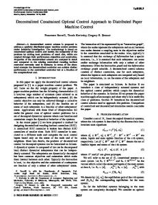
Fig. 3 Contours of p ¡ pa at four equally spaced instants, spanning one period of oscillation Tp (six equally spaced contour levels between § 7:0 £ 10¡6 ).
has uniform spacing of 1x1 D 1x2 D 0:05. Because the line source is harmonic, and the effect of nonlinearitiesaway from the source region is negligible, the ow eld exhibits a limit-cycle behavior with period T p as t ! 1. The initial time t0 is chosen large enough for this limit-cycle pattern to be established effectively in the domain. Figure 3a shows contours of pressure uctuations about the ambient pressure, p ¡ pa , for the uncontrolled ow within one period of oscillation.
The analytical solution for the in nite-dimensional no-control problem can be found easily by superimposition of an image line source at x2 D ¡H . The second component of velocity v2 and pressure p can be written as
£
¡
v2 D 4vm sin.2¼ x 2 / cos 2¼ H ¡ t C
1 4
p D 4 pm cos.2¼ x2 / cos[2¼.H ¡ t/]
¢¤
(21a) (21b)
1263
COLLIS, GHAYOUR, AND HEINKENSCHLOSS
a) Control g near the nal time tf
a) x = 0
b) At time t = 40.5, poptimal ¡ pnocontrol (20 evenly spaced contours between § 3:5 £ 10¡6 )
b) x = 0, § 1/4
Fig. 4 Effect of control for case 1.
In Eqs. (21), the velocity and pressureamplitudeof the harmonic line source are denoted by vm and pm , respectively.Equation (21a) satis es the inviscid wall boundary condition at x2 D 0 at all times. Further examination of Eq. (21b) shows that, for t D H=c C .2n C 1/=4, n D 0; 1; 2; 3; : : : , the pressure uctuation vanishes everywhere in the domain. This behavior is seen in the second and fourth plots of Fig. 3a. For this test case, the value of the objective function (7) at the initial iterate g0 D 0 (no control) is J .g0 / D Jobs .g0 / D 1:2 £ 10¡3 . After 15 nonlinear conjugate gradient iterations,2 the computed control g15 reduces the observation term in the objective function to Jobs .g15 / D 6:6 £ 10¡4 , which is about 45% of its initial value. Because of our choice of weights ®i , we obtain that Jreg .g15 / ¼ 10¡10 Jobs .g15 /, that is, the value J .g15 / of the objective function (7) can be equated with Jobs .g15 /. The same is also true for the other test cases. The acoustic pressure contours for the controlled run are shown in Fig. 3b. To analyze the behavior of the computed control, the time history of the control at x 1 D 0; § 14 is plotted in Fig. 5. Figure 5a depicts the time history of control at x 1 D 0. Note that the control has no dif culty in picking up the source frequency, and the control oscillates with an approximately constant amplitude for most of the time window .t0 ; t f /. Close to the nal time, the control loses the harmonic behavior and becomes approximatelyconstant. Figure 5b shows the time history of control at three locations on the wall, x 1 D 0; § 14 , separated by one-quarter wavelength. Figure 5b demonstrates that the controls at these three
Fig. 5
Time history of control g.
locations are exactly in phase. Further checks reveal that the control indeed is constant across the control region and is only a function of time. Because the lower edge of the observation region is located at a distance 12 above the wall, it takes about 12 time units for the effect of the boundary actuation to be felt in the observation region, explaining the behavior of the control near the nal time shown in Fig. 4a. From t D 49:5 onward, the control cannot affect the observation term, and, hence, it tries to minimize the contribution of the regularization term. The contribution of the spatial derivatives gx 1 and g x 1 x1 to Eqs. (7) is zero, and the contribution of the time regularization term kgt k22 is approximately 4¼ 2 ¼ 39:5 times larger than the regularizationterm kgk22 for a simple harmonic oscillation. Therefore, the main focus of the optimal control in the time period .39:5; t f / is to reduce gt initially, which is clearly achieved by creating a plateau near the nal time t f . To understand the effect of the computed control, one can subtract the uncontrolled pressure eld from the optimal control pressure eld as shown in Fig. 4b. Because the amplitude of ow quantities are small, the nonlinear terms in the governing equations are negligible and the contour plot of Fig. 4b isolates the effect of boundary actuation. Note that the boundary control creates a nearly planar wave to counter the wave system (21) in the observation region. A perfect cancellation is not possible because the wave produced by the control cannot cancel the wave system (21) at all times. The optimal control targets instants of time at which the observation region has high-amplitude waves (the rst and third snapshots of Fig. 3a) and tries to reduce
1264
COLLIS, GHAYOUR, AND HEINKENSCHLOSS
these waves by producing the wave shown in Fig. 4b. The control slightly disturbs the approximately silent instants observed in the second and fourth plots of Fig. 3b. Test Case 2
In this test case, we control the scattered and refracted wave pattern arising from the interactionof a monopole sound source with an inviscid vortex. Again, all ow quantities are nondimensionalized
a) No control Fig. 6
b) Optimal control
with source period T p and acoustic wavelength L. The monopole sound source, modeled as a source term in the energy equation, is located at .0; 5/ and interacts with an inviscid vortex31 of circulation 2¼=5 (counterclockwise) and radius 12 located at .0; 3:5/. The computational domain, control objective, and the spatial and temporal discretizationsare identical to that of test case 1. Sponge-type nonre ecting far- eld boundary conditions are now used on the left, right, and top boundaries. The distance between the vortex and the
c) Far- eld BC on bottom boundary
Contours of p ¡ pa at four equally spaced instants, spanning one period of motion Tp (six contour levels between § 1:75 £ 10¡4 ).
1265
COLLIS, GHAYOUR, AND HEINKENSCHLOSS
solid wall is large enough to ignore the effect of the image vortex in the optimization time interval comfortably. Hence, the vortex is considered to be stationary and the mean ow pressure distribution to be steady. The time interval comprises 600 uniform time steps of size 1t D 0:025 from time t0 D 30 to time t f D 45. Again, the initial time is larger than the time required for the limit-cycle pattern to be established effectively in the domain. After 20 optimization iterations, the control objective is reduced from Jobs .g0 / D 0:49 to Jobs .g20 / D 0:34. The acoustic pressure contours for the no-control and optimal-control simulations are shown in Figs. 6a and 6b, respectively. In the no-control simulation, the scattered wave behind the vortex is mostly observed in the right half of the observation region, which is due to the counterclockwise circulation of the vortex. The left half is relatively silent. The solid wall intensi es the incident waves and forces the waves to move horizontally. However, focus shifted onto the observation region of the optimal control run reveals that the main difference between the two runs is the slanted contours of the optimal control simulation. To understandthe control mechanism, another simulation is performed where the solid wall is replaced with a nonre ecting boundary condition based on Riemann extrapolation.Figure 6c shows four snapshots of the acoustic pressure eld at the same instants in time by the use of the Reimann boundary treatment. The pressure contours in the observation region for this run are very similar to that of the optimal control run, both slanting at an angle to the horizon, unlike the almost at contours of the uncontrolled run. This suggests that the optimal control attempts to mimic an absorbing boundary. The computed optimal control makes the wall nearly transparent to the incident waves, thereby preventing them from re ecting and intensifying the sound measured in the observation region. In the no-control run, the refracted/re ected wave pattern seen in the middle of the observation region is approximately horizontal. However, the wave system produced by the boundary actuation (Fig. 7b) and the wave pattern observed in the center of the optimal control plots (Fig. 6) slant in opposite directions. The production of the slanted wave of Fig. 7b by the boundary actuation is further validated by Fig. 7a, where the time history of control at three positions, x 1 D ¡0:25; 0, and 0.25, separated by one-quarter acoustic wavelength, is plotted. The phase difference in control actuation at these three locations allows for the production of waves with slanted fronts. Note that the control amplitude is smaller at x 1 D ¡0:25 than at the other two locations. This shows that the optimal control avoids disturbing the relatively silent left half of the observation region while attenuating the noisy right half of this region. Test Case 3
In test case 2, we argued that the computed transpirationboundary actuation effectively rendered the controlled surface transparent to incident waves. Test case 3 allows us to quantify how closely a transpirationwall is capableof mimickinga nonre ectingboundarycondition. The computational domain is Ä D [¡12; 12] £ [0; 14], with periodic boundary conditions enforced in the horizontal direction and a sponge nonre ecting boundary treatment in the vicinity of the top boundary.The control objectiveis identicalin form to that of the preceding test cases and is de ned over Äobs D [¡5; 5] £ [5; 9] and time horizon [2; 9], comprising 175 uniform time steps 1t D 0:04. The spatialmesh .241 £ 141/ has uniform spacing1x 1 D 1x 2 D 0:1 in both directionsand transpirationcontrol is allowed over the entire bottom boundary. The initial condition is a Gaussian acoustic pulse of amplitude ² D 10¡3 , with standard deviation ¾ D 0:25, centered at mean height x2¤ D 8 above the wall: v1 D 0;
©
v2 D ¡.²=2/ exp ¡ 12
p ¡ pa D ¡½a ca v2 ;
£¡
x 2 ¡ x2¤
¢¯ ¤2 ª ¾
¯
½ ¡ ½a D . p ¡ pa / ca2
(22)
In Eqs. (22), the subscript a denotes the ambient condition assumed to be a uniform quiescent ow where ½a D Ta D 1 and ca D 2. The
a) Time history of control g at x1 = 0, § 14
b) At time 40.75, poptimal ¡ pnocontrol (20 contours between § 9:0 £ 10¡5 ) Fig. 7
Effect of control for case 2.
acoustic pulse propagates at the ambient speed of sound ca D 2 toward the wall, and, at t0 , the beginning of the optimization horizon, it is located at x 2 D 4. For the no-control simulation, the pulse re ects off of the solid wall, passes through Äobs , and reaches x 2 D 10 at the nal time t f . We use ®0 D 106 , ®1 D 10¡3 , ®2 D 10¡4 , and ®3 D ®4 D 10¡3 . Optimization starts at the no-control con guration with J .g0 / D Jobs .g0 / D 9:19 £ 10¡1 , kr J .g0 /kG D 3430 and is terminated after 133 nonlinear conjugate gradient iterations Jobs .g133 / D 3:98 £ 10¡5 , kr J .g133 /kG D 2:59. The norm, kgkG , which is speci ed in Ref. 2, is related to
Z t fZ t0
0c
g 2 C gt2 C jr gj2 C j1gj2 d0 dt
and is not the Euclidean norm. Four snapshots of the acoustic pressure contours of the no-control and optimally controlled ow are shown in Fig. 8. We note that, whereas the uncontrolled ow is one dimensional,the controlled ow is two-dimensionaldue to the nite sized control region on the bottom wall. Figure 8a shows that the observation region is quiet except for the time interval in which the re ection off of the solid wall passes through it. Therefore, the optimal control actuation can not decrease the objective function unless it eliminates the re ection from the wall and makes the controlled wall transparent to the incident acoustic pulse. This behavior is evident in Fig. 8b, where the
1266
COLLIS, GHAYOUR, AND HEINKENSCHLOSS
a) No control Fig. 8
b) Optimal control
Contours of p ¡ pa at instants t = 2, 4, 8, and 9 (41 contour levels between 8:12 £ 10¡6 and 4:74 £ 10¡4 ).
control actuation has allowed the central portion of the acoustic pulse between [¡5; 5] to pass through the wall without noticeable re ection. To access the performance of the optimal control transpiration boundary condition (BC) in producing an essentially nonre ecting boundarycondition,we remove the lower wall and enforce the wellknown nonre ecting treatments: 1) Riemann extrapolation and 2) sponge. Then we compute
Jobs D
1 2
Z tZf t0
Äobs
®0 . p ¡ pa /2 dx dt;
®0 D 106
for each case, to estimate the amount of re ections produced by each boundary treatment. For the optimal transpiration boundary control, we nd that Jobs ¼ 4 £ 10¡5 , Riemann extrapolation BCs give Jobs ¼ 6:4 £ 10¡5 , and sponge BCs lead to Jobs ¼ 1: £ 10¡6 .
1267
COLLIS, GHAYOUR, AND HEINKENSCHLOSS
Fig. 9
Time history of pressure uctuations at (0; 7) for case 3.
We note that the Riemann condition performs somewhat worse than the spongebecauseRiemann treatmentsare well known to re ect the nonsmooth, numerical error waves. The amount of re ections in the observation region for the controlled wall is less than the Riemann treatment, whereas it is considerably higher than the sponge treatment. Because the transpiration and Riemann BC implementations are both based on the ow characteristics,the Riemann BC is a reasonablereferenceagainstwhich the performanceof the transpiration BC can be measured. That the optimal control boundary performs slight better than the Reimann BC is likely due to the numerical error associatedwith extrapolationin the Reimann BC. Figure 9 compares the amplitudes of the re ected waves by plotting the time history of pressure uctuations in the center of the observation region. The maximum sound amplitude for the optimal control simulation is slightly less than one-half of the peak re ection amplitude due to the Riemann treatment, whereas the peak re ection amplitude of the sponge treatment is about an order of magnitude smaller than the other two. Gradient Accuracy
As we have mentioned earlier, we use the optimize-thendiscretize approach to compute gradient information. That is, we rst derive adjoint equations and the objective function gradient on the PDE level and then discretize the resulting expressions. We denote the result by [r J .g/]h to indicate that discretization is performed after differentiation.The resulting derivative approximation differs from gradient r[Jh .g/]. It is obtained by discretization of the optimal control problem and then computation of the gradient of the resulting nite dimensional objective function Jh .g/. If adjoint computations are performed correctly, and if discretizations of state equation, objective function, and adjoint equations are chosen properly, one would expect that [r J .g/]h ¡ r[Jh .g/] ! 0 as the discretization level h is re ned. Moreover, the rate with which [r J .g/]h ¡ r[Jh .g/] goes to zero should be related to the approximation properties of the underlying discretization schemes. That, in fact, the convergence [r J .g/]h ¡ r[Jh .g/] ! 0 as h ! 0 is obtained is not at all straightforward. Even for optimal control problems far less complex than the one considered here, Refs. 32 and 33 offer some sobering results. The results in this section provide evidence that in our treatment [r J .g/]h ¡ r[Jh .g/] ! 0 as the discretization level h is re ned. Because we do not have access to the gradient of the discretized objective function Jh .g/, we choose an arbitrary unit direction ±g in the space of admissible controls and compare h[r J .g/]h ; ±giG with a nite difference approximation of hr[Jh .g/]; ±giG . Here, hg1 ; g2 iG is a weighted Euclidean norm corresponding to k kG , which is speci ed in detail in Ref. 2. To select a suitable nite difference step size ², we evaluate the discretized objective function
Fig. 10 Mesh re nement study for test case 3, showing approximate directional derivative (DA) and the fourth-order nite difference approximation to the directional derivative (DFD).
at §²±g and §2²±g and compare the second-order approximation [Jh .g C ²±g/ ¡ Jh .g ¡ ²±g/]=.2²/ with a fourth-order nite difference approximation. The nite difference step size ² is varied until these two approximations agree to a relative error of less than 10¡6 (for test case 3). For example, for test case 3, which uses a 241 £ 141 grid and g D 0, the computed second-order approximation to hr[Jh .g/]; ±giG is ¡535:1712, and the computed fourthorder approximation is ¡535:1714. The corresponding directional derivative computed with the optimize-then-discretize approach is h[r J .g/]h ; ±giG D ¡535:1872. Figure 10 shows the results of grid convergence studies with grids ranging in size from 241 £ 141 to 961 £ 561. For our computations, the solution at the nest discretization 961 £ 561 is assumed to be the reference solution and is denoted by subscript f . In Fig. 10, three relative error measures have been plotted against the number of mesh points N x 1 , where N x 1 is the number of grid points in the x1 direction, and the number of grid points in the x 2 direction is .7=12/.N x1 ¡ 1/ C 1, chosen to give the same grid spacing in both directions. In Fig. 10, J denotes the value of the objective function (7a). The approximate directional derivative h[r J .g/]h ; ±giG is obtained by discretization of the adjoint equations (optimize then discretize), and the fourthorder nite difference approximation to the directional derivative hr[Jh .g/]; ±giG is obtained by differentiationof the discretized objective function. Both axes of Fig. 10 have a logarithmicscale, and the slope of each line measures the order of convergence as discretization is further re ned. The observed rate of convergencefor the objective function J is approximately 5:5, whereas the relative errors between the directional derivative approximations converge with an observed rate of approximately three. Because we use a nite difference scheme that is sixth-order accurate in the interior and third-order accurate near the boundary, because we apply a fourth-order time-stepping scheme, and because we employ sponge and Riemann extrapolation at the far eld, it is dif cult to conjecture what theoretical convergence rates should be obtained. However, our observed convergence rates for the various quantities are sensible. In particular, the comparison between the derivative information h[r J .g/]h , ±giG obtained from our optimize-then-discretize approach and the nite difference approximation to the directional derivative hr[Jh .g/]; ±giG of the discretize-then-optimize approach support our procedure.
Conclusions This work focuses on several important issues encountered in the optimal boundary control of aeroacoustic ows governed by high-order central nite difference discretizations of the unsteady
1268
COLLIS, GHAYOUR, AND HEINKENSCHLOSS
Euler equations. These issues include: proper resolution of uctuating ow quantities, nonre ecting far- eld boundary treatments, and solid wall modeling. The importance of these issues is well known for computational aeroacoustics, but they are also critically important when optimal control is applied to aeroacoustic ows. In addition, optimal transpiration boundary control of aeroacoustics also requires the formulation and implementation of accurate near eld BCs on the controlled segment of the boundary. It is argued, based on the characteristic wave propagation speeds normal to the controlledboundary,thatsubsonicsuctionrequiresone physicalBC, whereas blowing requires three physical BCs. Our implementation of the transpiration BC is based on a decomposition of the inviscid uxes into several planar pseudowaves aligned with the boundary tangent and boundary normal directions by the use of a technique originally introduced by Sesterhenn.1 The transpiration BC is applied to three optimal control test problems. A continuous adjoint gradient-based method is used to solve the optimization problems, and the adjoint equation, its end time condition, and BCs are stated and discussed. Despite the difference in the number of derived adjoint BCs for suction, blowing, and solid walls, the adjoint BCs are compatible because the control tends to zero. The rst test problem demonstrates that the transpiration control actuation is capable of producing well-resolved acoustic waves that reduce the observed sound amplitude by means of wave cancellation. In the second test problem, the transpiration BC mimics a nonre ecting BC on the controlled surface to eliminate the intensifying effect of re ections off of the solid wall. The nal test problem demonstrates that optimal transpiration control is capable of creating a nonre ecting surface that rivals the widely used Riemann nonre ecting far- eld treatment.
Derivation of the Adjoint Equations
We associate adjoint variables
¸1 B ¸2 C C ¸DB @ ¸3 A ; ¸4
0 01 ¸1
0 b1 ¸1
B C
¸b D @¸b2 A ; ¸b3
B 0C B¸ 2 C 0 C ¸ DB B¸ 0 C @ 3A
Z L.u; g; ¸; ¸ ; ¸ / D J .g/ C
Z C
tf
tf
0
¸04
t0
µ
Z T
Ä
¸ q.u/t C
Z
t0
0
2 X
tf
Z
Z
tf
0 T
t0
Ä
.u / r C
Z C
tf t0
.¸/ t0
¶ i
F .u/ x i dx dt
i D1
.¸ / .u ¡ u0 / dx
0
b
0
0
.¸b / T Bu u0 C
D J .g/g D D g L.u; g; ¸; ¸ ; ¸ /g
Z
tf
t0
C
Ä
.u0 / T ¸0 D 0
Z C
tf t0
0
.®1 gt gt0 C ®2 gg 0 C ®3 r grg 0 C ®4 1g1g 0 / dx dt
Z 0
.¸b / T Bg .u; ru; g/g 0 dx dt
X
¶
i
0
.A u /x i
i
´ Bu xi u0xi
i
8u0
(A3)
In Eq. (A3), r is de ned by Eq. (9). Integration by parts in Eq. (A3) and variation over all functions u0 leads to the equations M T ¸t C
X i
T
Ai ¸dxi D r;
¸ D 0;
.t0 ; t f / £ Ä
X j
X i
n j BuTx ¸b D 0; j
T
n i Ai ¸d C BuT ¸b ¡ @s
(A4a)
ft f g £ Ä
¸0 ¡ .M T ¸/jt D t0 D 0;
X
ft0 g £ Ä
(A4c)
.t0 ; t f / £ 0
(A4d)
s j BuTx ¸b D 0; j
j
(A4b)
.t0 ; t f / £ 0 (A4e)
(A2)
(A5)
¸b2 and ¸b3 are not needed. In the following, we derive the adjoint BCs for ¸ determined by Eqs. (A4d) and (A4e), as well as the relation between ¸ and ¸b1 speci ed by the same equations. Equations (11–13) state the adjoint BCs in terms of the adjoint variables ¸. For the derivation of these conditions and for their implementation, it is convenient to introduce the characteristic adjoint variables ª, which will be de ned hereafter. By M D @q=@u, we denote the Jacobian of the conservative variables with respect to the primitive variables. We recall that Ai D @Fi =@u. Hence, Ai D @Fi =@qM. It is well known (see, for example, Sec. 16.5.2 in Ref. 30) that ni
Z
0c
X
X ³ @Fi ´ (A1)
0
.Mu /t C
³
Z
i 0 T
0
Z
.¸b / T B.u; ru; g/ dx dt
The derivative D J .g/ of the objective function (7) applied to g 0 is given by
D
T
Ä
Z C
µ
Z
.¸b / T Bg .u; ru; g/ D ¡¸b1
with the Euler equation (3a), its BCs (3b), and initial conditions (3c), respectively. The Lagrangian corresponding to Eqs. (3a–3c) and (7) is b
Z
where, as before, s D .s1 ; s2 / T D .¡n 2 ; n 1 /T is the unit tangential vector. For additional details on the derivation of Eqs. (A4a–A4e), see Ref 3. Equation (A4a) gives the adjoint PDE for ¸, Eq. (A4b) speci es the nal time condition for the adjoint PDE, and Eqs. (A4d) and (A4e) determine the BCs for ¸. The Eqs. (A4d) and (A4e) also determinethe relationbetween the adjointvariables¸ and ¸b . Recall that ¸ b is needed for the computation of the derivative (A2) of the objective functional. In fact, because
Appendix: Adjoint Equations and Gradient of the Objective Function
0 1
where ¸, ¸b , and ¸0 are the solution of the adjoint equations Du L.u; g; ¸; ¸b ; ¸0 /u0 D 0 for all u0 . That is,
@q
D P¤P¡1
where ¤ is a diagonal matrix with diagonal entries vT n, v T n, v T n C c, vT n ¡ c, and
2
1
6 6 6v 6 1 6 PD6 6 v2 6 6 4vT v 2
0
½ 2c
¡½n 1
½ .v1 C cn1 / 2c ½ .v2 C cn2 / 2c
½ .v1 n 2 ¡ v2 n 1 /
½ .H C c vT n/ 2c
½n 2
½ 2c
3 7
7 ½ .v1 ¡ cn1 / 7 7 2c 7 7 ½ .v2 ¡ cn2 / 7 7 2c 7 5
½ .H ¡ c vT n/ 2c (A6)
1269
COLLIS, GHAYOUR, AND HEINKENSCHLOSS
p Here, c D .° p=½/ denotes the speed of sound, and H D 12 v T v C c 2 =.° ¡ 1/ is the stagnation enthalpy. With
2
L¡1
° ¡ 1=°
6 0 D P¡1 M D 6 4 c=° p c=° p
0 n2 n1 ¡n 1
0 ¡n 1 n2 ¡n 2
3
¡½=° T 0 7 7 c=° T 5 c=° T
(A7)
Solid Surface (vT n = g = 0)
On a uncontrolled solid surface, Eqs. (A11) and (A13) are identically satis ed, and only Eq. (A12) needs to be imposed. Blowing (v T n = g < 0) In the case vT n D g < 0, the BC operator and its derivatives are
given by
2
X i
T
n i Ai D M T
X ³ @Fi ´T ni
@q
i
D M T .P¤P¡1 / T D L¡T ¤PT
2
0 Bu D 4 ¡g 2 =½ 0
(A8)
This identity, together with the de nition ª D PT ¸
(A9)
2
of the characteristic adjoint variables will be used to rewrite (A4e). References 16 and 34–36 have also used adjoint characteristic variables in the formulation and implementation of adjoint BCs. Because the number of imposed BCs and the imposed quantities themselves depend on the sign of the normal velocity control, we discuss suction and blowing BCs separately.
Bu x j
n2
0 0
0 0
0 0 ±2 j g 2
3
0 g 2 =.° ¡ 1/T 5 0 0 0 ¡±1 j g 2
3
0 05 0
2
3
0 4 Bu D 0 0
n1 0 0
n2 0 0
2
3
0 05 ; 0
6 6 C6 6 4
Bu x j D 0
By the use of Eqs. (A8) and (A9), the Eqs. (A4e) are given by c °p n1 n2 c °T
3
c 2 3 2 0 3 0 vT nÃ1 °p 7 7 6 b7 vT nÃ2 7 6n 1 ¸1 7 n2 ¡n 1 7 6 7C6 76 7D0 ¡n 1 ¡n 2 7 4.vT n C c/Ã3 5 4n 2 ¸b 5 1 5 c .vT n ¡ c/Ã4 0 0 °T °T (A10) Multiplication of the rst equation in Eqs. (A10) by p, and subtraction from the result T times the fourth equation, leads to .vT n/Ã1 D 0
(A11)
The fourth equationof Eqs. (A10) and (A11) give the second adjoint BC .vT n C c/Ã 3 C .vT n ¡ c/Ã4 D 0
(A12)
If we multiply the second and third components of Eqs. (A10) by n 2 and ¡n 1 , respectively, and add the results, we obtain .vT n/Ã2 D 0
(A13)
Equations (A11–A13) are the adjoint BCs (11) stated earlier. If we multiply the second component of Eq. (A10) by n 1 , and the third component by n 2 , and add the results, we obtain ¸b1 D .vT n ¡ c/Ã 4 ¡ .vT n C c/Ã3
(A14)
The adjoint variable ¸b1 is the only component of ¸b needed for the computation of the objectivefunction derivative.[See Eqs. (A2) and (A5).]
(A15)
Equations (A15), (A8), and (A9) can be used to write Eq. (A4e) as ° ¡ 1=° 6 0 6 4 0 ¡½=° T
n 1 v1 C n 2 v2 ¡ g 5 0 B.u; ru; g/ D 4 0
2
¸b3 D 0
2
= g > 0)
The suction BC operator and its derivatives are given by
2° ¡ 1 6 ° 6 6 0 6 6 0 4 ¡½
0 D 40 0
n1
where ±i j denotes the Kronecker symbol. Equation (A4e) implies
Adjoint Wall BCs
Suction (v T n
3
n 1 v1 C n 2 v2 ¡ g 4 .S ¡ S0 /g 2 5 B.u; ru; g/ D .@ x 2 v1 ¡ @x1 v2 /g 2
we obtain
0 n2 ¡n 1 0
c=° p n1 n2 c=° T
¡.g 2 =½/¸b2 n 1 ¸b1 n 2 ¸b1
32
3
c=° p vT nÃ1 7 6 ¡n 1 7 6 vT nÃ2 7 7 ¡n 2 5 4 .v T n C c/Ã 3 5 c=° T .v T n ¡ c/Ã 4
3
7 7 7D0 7 5
(A16)
[g 2 =.° ¡ 1/T ]¸b2
Notice that the second and third components in Eq. (A16) are identical to the second and third components in Eq. (A10). Hence, we obtain Eqs. (A13) and (A14). Another BC for ¸ is obtainedfrom Eq. (A16). We can eliminate¸b2 from the rst and fourth components of Eq. (A16) by multiplying these components by ½ and .° ¡ 1/T , respectively, and add the results to obtain .v T n C c/Ã 3 C .vT n ¡ c/Ã4 D 0
(A17)
In summary, there are two BCs thatneed to be imposedon Ã, namely, Eqs. (A17) and (A13). These BCs are equivalent to Eq. (A13). As in the preceding case, the adjoint variable ¸b1 needed for the computation of the objective function derivative [see Eqs. (A2) and (A5)] is obtained from Eq. (A14). Note that the vorticity BC of the state only leads to the condition (A15). Because it involves only derivatives of the primitive variables, this BC does not enter Eq. (A16). A consequence of this is the appearance of the additional BCs (A13). Gradient Computation
Given ¸b1 , the gradient of the objective function can now be computed from Eq. (A2). Details may be found in Ref. 2.
Acknowledgments This work was supported in part by Texas Advanced Technology Program Grant 003604-0001-1999, National Science Foundation (NSF) Grant DMS-0075731, and the Los Alamos National Laboratory (LANL) Computer Science Institute through LANL Contract 03891-99-23 as part of the prime contract (W-7405-ENG-36) between the Department of Energy and the Regents of the University of California.Computationswere performed on an SGI Origin 2000, which was purchased with the aid of NSF Grant 98-72009.
1270
COLLIS, GHAYOUR, AND HEINKENSCHLOSS
References 1 Sesterhenn, J., “A Characteristic-Type Formulation of the Navier – Stokes
Equationsfor High Order Upwind Schemes,” Computers and Fluids, Vol. 30, 2001, pp. 37– 67. 2 Collis, S. S., Ghayour, K., Heinkenschloss, M., Ulbrich, M., and Ulbrich, S., “Optimal Control of Unsteady Compressible Viscous Flows,” International Journal on Numerical Methods in Fluids, Vol. 40, 2002, pp. 1401– 1429. 3 Collis, S. S., Ghayour, K., Heinkenschloss, M., Ulbrich, M., and Ulbrich, S., “Numerical Solution of Optimal Control Problems by the Compressible Navier– Stokes Equations,” Proceedings of the International Conference on Optimal Control of Complex Structures, edited by G. Leugering, J. Sprekels, and F. Tr¨oltzsch, Vol. 139, Birkh¨auser Verlag, Oberwolfach, Germany, 2001, pp. 43– 55. 4 Collis, S. S., Ghayour, K., and Heinkenschloss, M., “Optimal Control of Aeroacoustic Noise Generated by Cylinder Vortex Interaction,” International Journal of Aeroacoustics, Vol. 1, 2002, pp. 97 – 114. 5 Tam, C. K. W., and Dong, Z., “Wall Boundary Conditions for HighOrder Finite Difference Schemes in Computational Aeroacoustics,” Theoretical and Computational Fluid Dynamics, Vol. 6, No. 6, 1994, pp. 303– 322. 6 Kurbatskii, K. A., and Tam, C. K. W., “Cartesian Boundary Treatment of Curved Walls for High-Order Computational Aeroacoustics Schemes,” AIAA Journal, Vol. 35, No. 1, 1997, pp. 133– 140. 7 Joslin, R. D., Gunzburger, M. D., Nicolaides, R. A., Erlebacher, G., and Hussaini, M. Y., “Self-Contained Automated Methodologyfor Optimal Flow Control,” AIAA Journal, Vol. 35, No. 5, 1997, pp. 816– 824. 8 Abergel, F., and Temam, R., “On Some Control Problems in Fluid Mechanics,” Theoretical and Computational Fluid Dynamics, Vol. 1, 1990, pp. 303– 325. 9 Berggren, M., “Numerical Solutionof a Flow-Control Problem: Vorticity Reduction by Dynamic Boundary Action,” SIAM Journal on Scienti c and Statistical Computing, Vol. 19, 1998, pp. 829– 860. 10 He, J.-W., Glowinski, R., Metcalfe, R., Nordlander, A., and Periaux, J., “Active Control and Drag Optimization for Flow Past a Circular Cylinder. I. Oscillatory Cylinder Rotation,” Journal of ComputationalPhysics, Vol. 163, 2000, pp. 83– 117. 11 Fursikov, A. V., Gunzburger, M. D., and Hou, L. S., “Boundary Value Problems and Optimal Boundary Control for the Navier – Stokes Systems: The Two-Dimensional Case,” SIAM Journal of Control and Optimization, Vol. 36, 1998, pp. 852– 894. 12 Gunzburger,M. D., and Manservisi, S., “The Velocity Tracking Problem for Navier– Stokes Flows with Boundary Control,” SIAM Journal of Control and Optimization, Vol. 39, 2000, pp. 594– 634. 13 He, B., Ghattas, O., and Antaki, J. F., “Computational Strategies for Shape Optimization of Time-Dependent Navier– Stokes Flows,” Dept. of Civil and Environmental Engineering, TR CMU-CML-97-102, Carnegie Mellon Univ., Pittsburgh, PA, June 1997. 14 Li, Z., Navon, M., Hussaini, M. Y., and Dimet, F. X. L., “Optimal Control of Cylinder Wakes via Suctionand Blowing,” Computers and Fluids, Vol. 32, No. 2, 2003, pp. 149– 171. 15 Anderson, W. K., and Venkatakrishnan, V., “Aerodynamic Design Optimization on Unstructured Grids with a Continuous Adjoint Formulation,” ICASE, TR 97-9, Hampton, VA, 1997. 16 Giles, M. B., and Pierce, N. A., “Adjoint Equations in CFD: Duality, Boundary Conditions and Solution Behavior,” AIAA Paper 97-1850, 1997.
17 Iollo, A., and Salas, M. D., “Optimum Transonic Airfoils Based on the Euler Equations,” ICASE, TR 96-76, Hampton, VA, 1996. 18 Jameson, A., and Reuther, J., “Control Theory Based Airfoil Design Using the Euler Equations,” AIAA Paper 94-4272, June 1994. 19 Nadarajah, S. K., and Jameson, A., “A Comparison of the Continuous and Discrete Adjoint Approach to Automatic Aerodynamic Optimization,” AIAA Paper 2000-0667, Jan. 2000. 20 Lele, S. K., “Compact Finite Difference Schemes with Spectral-Like Resolution,” Journal of Computational Physics, Vol. 103, No. 1, 1992, pp. 16– 42. 21 Tam, C. K. W., and Webb, J. C., “Dispersion-Relation-Preserving Finite Difference Schemes for Computational Acoustics,” Journal of Computational Physics, Vol. 107, 1993, pp. 262– 281. 22 Collis, S. S., “A Computational Investigation of Receptivity in HighSpeed Flow Near a Swept Leading-Edge,” Ph.D. Dissertation, Dept. of Mechanical Engineering, Stanford Univ., Stanford, CA, March 1997. 23 Carpenter, M. H., Gottlieb, D., and Abarbanel, S., “Stable and Accurate Boundary Treatments for Compact, High-Order Finite Difference Schemes,” Applied Numerical Mathematics, Vol. 12, No. 1– 3, 1993, pp. 55 – 87. 24 Israeli, M., and Orszag, S. A., “Approximation of Radiation Boundary Condition,” Journal of Computational Physics, Vol. 41, 1981, pp. 115– 135. 25 Thompson, K. W., “Time-Dependent Boundary Conditions for Hyperbolic Systems,” Journal of Computational Physics, Vol. 68, 1987, pp. 1– 24. 26 Thompson, K. W., “Time-Dependent Boundary Conditions for HyperbolicSystems, II,” Journal of ComputationalPhysics, Vol. 89, 1990,pp. 439– 461. 27 Poinsot, T. J., and Lele, S. K., “Boundary Conditions for Direct Simulations of Compressible Viscous Flows,” Journal of ComputationalPhysics, Vol. 101, No. 1, 1992, pp. 104– 129. 28 Giles, M. B., “Nonre ecting Boundary Conditions for Euler Equation Calculations,” AIAA Journal, Vol. 28, No. 12, 1990, pp. 2050– 2058. 29 Moretti, G., “The ¸-scheme,” Computers and Fluids, Vol. 7, 1979, pp. 191– 205. 30 Hirsch, C., Numerical Computation of Internal and External Flows, Vol. 2, Wiley, New York, 1990, Chap. 19. 31 Shu, C.-W., “Esentially Non-Oscillatory and Weighted Essentially NonOscillatory Schemes for Hyperbolic Conservation Laws,” ICASE, TR 97-65, Hampton, VA, Nov. 1997. 32 Hager, W. W., “Runge– Kutta Methods in Optimal Control and the Transformed Adjoint System,” Numerische Mathematik, Vol. 87, 2000, pp. 247– 282. 33 Vogel, C. R., and Wade, J. G., “Analysis of Costate Discretizations in Parameter Estimation for Linear Evolution Equations,” SIAM Journal on Control and Optimization, Vol. 33, 1995, pp. 227– 254. 34 Sanders, B. F., and Katopodes, N. D., “Control of Canal Flow by Adjoint Sensitivity,” Journal of Irrigation and Drainage Engineering, Vol. 125, No. 5, 1999, pp. 287– 297. 35 Sanders, B. F., and Katopodes, N. D., “Adjoint Sensitivity Analysis for Shallow-Water Wave Control,”Journal of Engineering Mechanics, Vol. 126, No. 9, 2000, pp. 909– 919. 36 Baysal, O., and Ghayour, K., “ContinuousAdjointSensitivities for General Cost Functionals on Unstructured Meshes in Aerodynamic Shape Optimization,” AIAA Journal, Vol. 39, No. 1, 2001, pp. 48 – 55.
W. J. Devenport Associate Editor