Optimum Monte Carlo Simulations: Some Exact Results

arXiv:cond-mat/0302366v1 [cond-mat.stat-mech] 18 Feb 2003

Optimum Monte Carlo Simulations: Some Exact Results J. Talbot1 , G. Tarjus2 and P. Viot2 1

Department of Chemistry and Biochemistry, Duquesne University, Pittsburgh, PA 15282-1530 2 Laboratoire de Physique Th´eorique des Liquides, Universit´e Pierre et Marie Curie, 4, place Jussieu, 75252 Paris Cedex, 05 France Abstract. We obtain exact results for the acceptance ratio and mean squared displacement in Monte Carlo simulations of the simple harmonic oscillator in D dimensions. When the trial displacement is made uniformly in the radius, we demonstrate that the results are independent of the dimensionality of the space. We also study the dynamics of the process via a spectral analysis and we obtain an accurate description for the relaxation time.

PACS numbers: 05.70.Ln,81.05.Rm,75.10.Nr,64.60.My, 68.43.Mn, 75.40.Gb

1. Introduction Since the original Metropolis algorithm appeared five decades ago, countless studies have employed the technique to evaluate the thermodynamic properties of model systems[Allen and Tildesley, 1987, Binder, 1997, Frenkel and Smit, 2002]. The essence of the method is to generate a sequence of configurations that represent a given thermodynamic ensemble, often the canonical ensemble. Properties of interest are then obtained as averages over the configurations. At each step of the simulation a trial configuration is obtained from the current one by making a random displacement in the configuration space. This might correspond to, for example, displacing a randomly selected particle. The trial configuration is either accepted or rejected with a probability given by the appropriate Boltzmann factor for the ensemble. In case of rejection, the current configuration is retained for use in evaluating the properties of interest. Since many applications of MC are computationally intensive, a much addressed issue has been the optimization of the simulation with respect to one or more control parameters so that the configuration space is sampled in the most efficient way. Bouzida, Kumar and Swendsen (BKS)[Bouzida et al., 1992, Swendsen, 2002], as part of a program aimed at improving the efficiency of MC simulations of biomolecules, performed numerical studies of the simple harmonic oscillator (SHO) where the convergence of the simulation depends on the maximum displacement. There is no unique measure of efficiency, but two simple choices are the mean squared and mean

Optimum Monte Carlo Simulations: Some Exact Results

2

absolute displacements. As the maximum displacement tends to zero or infinity it is clear that the average value of both of these quantities tends to zero since, in the first case the particle does not move, while in the second all attempted moves are rejected. Thus both quantities have a maximum for some intermediate value of the maximum displacement. It is also useful to consider the dynamical process associated with an MC simulation, even though it does not correspond to the actual dynamics of the system. One can, for example, calculate various time correlation functions that can be used to develop alternative efficiency criteria[Kolafa, 1988, Mountain and Thirumalai, 1994]. BKS[Bouzida et al., 1992] performed numerical studies of the SHO in one, two and three dimensions and examined the acceptance ratio Pacc (i.e., the fraction of accepted trial configurations), mean squared, < (∆x)2 ) >, and mean absolute, < |∆x| >, displacements as a function of the maximum displacement, δ. They found that the acceptance ratio decreases approximately exponentially for small to intermediate values of δ and then inversely for larger values. In one dimension they found that the maxima in < (∆x)2 > and < |∆x| > occur at Pacc = 0.42 and Pacc = 0.56, respectively. In higher dimensions the results depend on how the jump is made. BKS considered two cases: in one the jumps are performed uniformly to any point in a spherical volume of radius δ centered on the current position, a choice that favors larger radial displacements for dimensions D > 1. In a second method, the jumps were sampled uniformly in the radius (and randomly in the orientation) so that all radial displacements are equally probable. In the former case BKS observed that, for a given δ, Pacc decreases as a function of D, while for uniform radius sampling the numerical results suggested that Pacc is independent of D. In addition to these static properties, BKS also examined the correlation time, τ , of the energy-energy correlation function. They observed a minimum correlation time for an acceptance ratio of approximately 50%. Here we present an analytical study of the SHO in arbitrary dimension. We obtain exact expressions for the acceptance ratio and the mean squared and mean absolute displacements as functions of the maximum displacement δ. We show that when the trial jump is selected uniformly in the radius, the results are independent of the dimension. We also present an analysis of the dynamics of the process. 2. ONE DIMENSION We first investigate the case of a SHO in one dimension, whose potential energy is given by V (x) = kx2 /2 where x is the position and k is the stiffness constant. In a standard Metropolis Monte Carlo Simulation one makes a trial move with a uniform random displacement selected between −δ and δ. The dynamical process generated by the successive trial moves of the Monte Carlo simulation can be written 1 Zδ 1 Zδ dP (x, t) dhW (x → x + h)P (x, t) + dhW (x + h → x)P (x + h, t) =− dt 2δ −δ 2δ −δ

(1)

3


1

0.8

Pacc

0.6

0.4

0.2

0

0

2

4

ξ

6

8

10

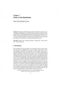
q βk Figure 1. Acceptance ratio Pacc versus ξ = 2 δ for a harmonic oscillator with uniform volume sampling in D = 1, 2, and 3 dimensions (full, dashed, and dotted lines respectively). For a uniform radius sampling, all curves coincide with the onedimensional result (full line).

where W (x → x + h) denotes the transition rate from the state x to the state x + h and P (x, t) is the probability to find the oscillator at position x at time t. To ensure the convergence towards equilibrium, a sufficient condition is given by detailed balance, which is expressed as Peq (x + h) W (x → x + h) = W (x + h → x) Peq (x)

where

(2)

Peq (x) = c exp(−βV (x)) q

and c = βk/2π is a normalization constant ensuring that solution of Eq. (2) is the Metropolis rule,

(3) R∞

−∞

W (x → x + h) = min(1, exp(−β(V (x + h) − V (x))).

dxPeq (x) = 1. One (4)

Most of the properties of the 1D SHO can be obtained analytically. For instance, the acceptance ratio, which is the number of accepted trials over the total number of trials can be expressed as Z δ Z +∞ −βV (x) 1 dhW (x → x + h). (5) dxe Pacc (δ) = c 2δ −δ −∞

4


0.8

0.4

2

(β κ) /2

0.6

0.2

0

0

0.2

0.4

0.6

0.8

1

Pacc

Figure 2. Mean squared displacement < (∆r)2 > βk 2 versus the acceptance ratio Pacc for uniform volume sampling in one, two and three dimensions (full curve, dashed, and dotted lines, respectively). For a uniform radius sampling all curves coincide with the one-dimensional result (full line).

In this equation exp(−βV (x))dx is the probability that the oscillator is between x and x + dx, dh/2δ is the probability of selecting a random displacement between h and h + dh and W (x → x + h) is the probability of accepting the trial displacement (given by Eq. (4)). Integration over the allowed values of x and h then gives the average acceptance probability. Since displacements to the left and right are symmetric, we need consider only one direction. For displacements to the right, Eq. (5), can be written as Z +∞ d(δPacc (δ)) =c dxe−βV (x) W (x → x + δ). (6) dδ −∞ 2 −x2 )/2

For x < −δ/2, W (x → x + δ) = 1 and for x > −δ/2, W (x → x + δ) = e−βk((x+δ) One thus obtains ! ξ d(ξPacc(ξ)) = 1 − erf dξ 2

.

(7)

q

δ. Using the initial condition, i.e., where erf (x) is the error function and ξ = βk 2 Pacc (0) = 1, the solution of the differential equation (7) is Pacc (ξ) = 1 − erf The function is plotted in Fig. 1.

!

2 ξ 2 +√ 1 − e−ξ /4 . πξ 2

(8)

5


0.5



⋅√(β κ) /2

0.4

0.3

0.2

0.1

0

0

0.2

0.4

0.6

0.8

1

Pacc

q Figure 3. Mean absolute displacement < |∆r| > βk 2 versus the acceptance ratio Pacc for a uniform volume sampling in one, two and three dimensions (full curve, dashed, and dotted lines, respectively). For a uniform radius sampling all curves coincide with the one-dimensional result (full line).

The mean squared displacement, < (∆x)2 >, and the mean absolute displacement, < |∆x| >, defined as

1 δ dhh2 W (x → x + h), (9) 2δ −∞ −δ Z +∞ Z 1 δ dx exp(−βV (x)) dh|h|W (x → x + h). (10) < |∆x| > = c 2δ −δ −∞ can be quite simply obtained from the generating function Z +∞ 1 Zδ dh exp(−λ|h|)W (x → x + h), (11) Z(λ) = c dx exp(−βV (x)) 2δ −δ −∞ by the derivatives with respect to λ and set λ = 0, i.e., < |∆x| >= −(∂Z(λ)/∂λ)λ=0 , < (∆x)2 >= (∂ 2 Z(λ)/∂λ2 )λ=0 (and, of course, Pacc = Z(λ = 0)). By multiplying both sides of Eq. (11) by ξ and next differentiating with respect to ξ, one obtains < (∆x)2 > = c

Z

+∞

dx exp(−βV (x))

s

∂(ξZ(λ, ξ)) 2 = exp − λξ ∂ξ βk ˜= which, after defining λ "

q

2 λ, βk

!

1 − erf

Z

ξ 2

!!

(12)

leads to

1 ˜ Z(λ, ξ) = 1 − exp(−λξ) 1 − erf ˜ λξ

ξ 2

!!

˜ 2 ) erf − exp(λ

!

ξ ˜ ˜ + λ − erf (λ) 2

!#

(13)

6


By taking the derivatives of the above formula with respect to λ and evaluating the resulting expressions at λ = 0, it is easy to show that the mean squared and mean absolute displacements are given by s



βk ξ 1 − erf < |∆x| >=  2 2

ξ 2

!!

"

βk 1 2 ξ 1 − erf < (∆x)2 >= 2 3

ξ 2

1 ξ2 − √ exp − π 4

!!

!

+

 ξ 2

erf

ξ

,

8 ξ2 ξ2 +√ 1− 1+ exp − πξ 4 4 !

(14) !!#

.

(15)

The maximum in the mean squared and mean absolute displacements occur for ξ = 2.61648 and ξ = 1.76332, which corresponds to acceptance ratio values of Pacc = 0.41767 and Pacc = 0.558239 in agreement with the numerical results of BKS[Bouzida et al., 1992]: see Figs. 2 and 3. 3. D dimensions We show here that the acceptance ratio, mean squared displacement and other quantities of interest can be obtained exactly in any dimension. Note that the term “volume” should be interpreted as the hypervolume in D dimensions, e.g., area in 2D and volume in 3D. For simplicity, we derive exact expressions in odd dimensions, but similar results can be obtained in even dimensions. 3.1. Uniform volume sampling In D dimensions, the acceptance ratio is expressed as Z cD Z D 2 d r exp(−βkr /2) dD h min(1, exp(−βk(|r + h|2 − r 2 )/2)) (16) Pacc (δ) = D δ VD |h|≤δ where VD = π D/2 /Γ(D/2 + 1) is volume of the sphere of unit radius in D dimensions and

cD = DVD

Z

0

∞

drr

D−1 −βkr 2 /2

e

−1

=

βk 2π

!D/2

.

(17)

In odd dimensions, the derivative of Eq. (16) with respect to δ can be written explicitly by using generalized spherical coordinates cD d(δ D Pacc (δ)) = dD r exp(−βkr 2 /2) dδ VDZ δ D−1 dΩ min(1, exp(−βk(rδ cos φ1 + δ 2 /2))), Z

(18)

D−1−j where dΩ = ( D−2 dφj )dφD−1 such that dΩ = DVD . The first D − 2 j=1 (sin(φj )) variables φj are integrated from 0 to π, whereas φD−1 is integrated from 0 to 2π. If we denote u = cos(φ1 ), perform integration over φ2 . . . φD−1 , and introduce the variable

Q

R

7

Optimum Monte Carlo Simulations: Some Exact Results v=r

q

βk 2

Eq. (18) can be rewritten as

2 d(ξ D Pacc (ξ)) = Dξ D−1 D R 1 × 2 (D−3)/2 dξ Γ −1 du(1 − u ) 2

×

Z

+∞

0

v D−1 dve−v

2

Z

1

−1

du(1 − u2 )(D−3)/2 min(1, exp(−(2ξvu + ξ 2 )))

(19)

where min(1, exp(−(2ξvu + ξ 2 ))) = exp((−(2ξvu + ξ 2)) for v < ξ/2 with −1 < u < 1 and for v > ξ/2 with −ξ/(2v) < u < 1 and min(1, exp(−(2ξvu + ξ 2 ))) = 1 for r > ξ/2 R1 Γ( D−1 ) √ π, Eq. (19) then with −1 < u < −ξ/(2v). Using that −1 du(1 − u2 )(D−3)/2 = Γ D2 (2) becomes Z ξ/2 Z 1 d(ξ D Pacc (ξ)) 2Dξ D−1 2 D−1 −v = √ (D−1) dvv e du(1 − u2 )(D−3)/2 exp(−(ξ 2 + 2ξvu)) dξ 0 −1 πΓ 2

+∞

+

Z

+

Z

ξ/2

v

D−1

1

−ξ/(2v)

−v2

dve

"Z

−ξ/(2v)

−1

2 1/2

du(1 − u )

du(1 − u2 )(D−3)/2 + #!

2

exp((−(ξ + 2ξvu)))

.

(20)

After some calculation (see Appendix A) one obtains, d(ξ D Pacc (ξ)) = Dξ D−1 1 − erf dξ

ξ 2

!!

(21)

which gives, for instance, in three dimensions Pacc (ξ) = 1 − erf

ξ 8 ξ2 ξ2 + √ 3 1− 1+ exp − 2 πξ 4 4 !

!

!!

(22)

Figure 1 shows the acceptance ratio Pacc versus δ in one, two and three dimensions. A similar calculation for generating function ZD (λ, ξ) leads to !! ˜ ξ)) ∂(ξ D ZD (λ, ξ ˜ D−1 −λξ , (23) 1 − erf = Dξ e ∂ξ 2 and to D−1 1−D ∂ ˜ ξ), ˜ Z (λ, (24) ZD (λ, ξ) = D(−ξ) ˜ D−1 D=1 ∂λ ˜ ξ) is given in Eq. (13). Since Pacc (ξ) = ZD (λ ˜ = 0, ξ), where the expression for ZD=1 (λ, it follows from Eq. q (24) that the acceptance ratio in D dimensions is equal, up a 1−D βk factor D(−ξ) , to the mean squared displacement < (∆x)2 > in one dimension: 2 compare Eq. (22) to Eq. (15). Although straightforward, the algebra rapidly becomes tedious, and we only illustrate the results by giving the expression of the mean squared displacement < (∆r)2 > in three dimensions

∂2 βk ˜ ξ)| ˜ < (∆r)2 > = Z (λ, λ=0 ˜ 2 D=3 2 ∂λ !2 3 βk < (∆x)4 >D=1 = 2 ξ 2

8

Optimum Monte Carlo Simulations: Some Exact Results 12 ξ 2 1 − erf = 5 4 "

ξ 2

!!

!

16 ξ2 ξ4 + √ 2 1− 1+ e + πξ 4 32

2

− ξ4

!#

. (25)

The mean squared and mean absolute displacement are plotted versus the acceptance ratio Pacc in one, two and three dimensions in Figs. 2 and 3. Note that the maximum is shifted to the left, i.e., to the smallest values of the acceptance ratio, when the space dimension increases. 3.2. Uniform radius sampling The acceptance ratio Pacc,w in D dimensions can be expressed as Pacc,w (δ) = cD Z

|h|≤δ

Z

D

dD r exp(−βkr2 /2)

dD hPw (h) min(1, exp(−βk(|r + h|2 − r 2 )/2))

(26)

where Pw (h) is the weighted probability. For a uniform distribution in radius, hD−1 Pw (h) = (DVD δ)−1 . Using the method developed in the above section, it is straightforward to obtain that d(ξPacc,w (δ)) = 1 − erf dξ

ξ 2

!!

(27)

which shows that the acceptance ratio is the same whatever the dimension and explains the data collapse observed in [Bouzida et al., 1992]. Similarly, the generating function Z(λ, ξ) can be shown to obey to the differential equation s

2 ∂Z(λ, ξ) = exp(− λξ) 1 − erf ∂ξ βk

ξ 2

!!

,

(28)

independently of the dimension D. This proves that Z(λ, ξ) and all moments such as < |∆r| > and < (∆r)2 > are independent of dimension, as numerically found by BKS[Bouzida et al., 1992]. 4. Dynamic behavior In addition to the exact results for the static properties presented above, we have investigated the dynamic behavior of the SHO by using numerical and analytical approaches. For simplicity, we discuss only the unidimensional case, but the approach can be generalized to D dimensions. The master equation describing the dynamical evolution of the system during the Monte Carlo simulation, Eq. (1), can be formally written dP(t) = −LP(t) (29) dt where L is a linear operator acting on P and the Metropolis rule, Eq (4), is used for the transition rate. We consider the spectrum of eigenvalues λ of L. Denoting Pλ (x) the


9

eigenfunction associated with λ and introducing fλ (x) via Pλ (x) = Peq (x)fλ (x), where Peq (x) is given in Eq. (3), one can express the eigenvalue equation λPeq (x)fλ (x) = L(Peq (x)fλ (x))

(30)

as 1 Zδ dhMin(1, e−β(V (x+h)−V (x)) )(fλ (x) − fλ (x + h)). (31) 2δ −δ Multiplying both sides by exp(−βV (x))fλ∗ (x), where the star denotes a complex conjugate, and integrating over x then gives λfλ (x) =

1 λ= 4δ

R +∞ −∞

dx

Rδ

−δ

dhMin(e−βV (x) , e−βV (x+h) )|fλ (x + h) − fλ (x)|2 . R +∞ −βV (x) |f (x)|2 λ −∞ dxe

(32)

As anticipated for a Markov process satisfying detailed balance, one deduces from the above formula that all eigenvalues are real and positive; the smallest eigenvalue is λ0 = 0 and it is associated with f0 (x) = constant 6= 0. One need consider only real eigenfunctions. Moreover, the eigenvalues can be sorted according to the symmetry of the associated eigenfunctions: it is easy to check that the eigenfunctions are either even or odd functions of x, due to the fact that the potential V (x) is an even function of x. Any solution of the master equation can be expanded as P (x, t) = Peq (x)(1 +

X

cλ fλ (x)e−λt ),

(33)

λ>0

and a similar expansion applies to the conditional probability P (x, t|x0 , 0) from which one can compute any time-dependent correlation function. The long-time kinetics governing the approach to equilibrium in P (x, t) and in any correlation function is characterized by the smallest non-zero eigenvalue for which the amplitude, i.e., the projection of P (x, 0), or of the dynamic observable, onto the relevant eigenfunction, does not vanish. Since, according to Eq. (32), the eigenvalues are expressed as the ratio of two positive quadratic functionals (that in the denominator being also definite), one can use the Rayleigh-Ritz procedure to find a variational upper-bound for the eigenvalues[Dettman, 1962, Arfken, 1985]. Consider first the smallest non-zero eigenvalue λ1 . For any real function φ(x) which is both normalized and orthogonal to f0 (x), i.e., satisfies Z

∞

−∞ Z ∞ −∞

Peq (x)φ(x)2 dx = 1

(34)

Peq (x)φ(x)dx = 0,

(35)

one has the inequality Z Z δ 1 +∞ dx dhMin(e−βV (x) , e−βV (x+h) )|φ(x + h) − φ(x)|2 . (36) λ1 ≤ λ1 [φ] = 4δ −∞ −δ A convenient choice of trial functions is provided by linearqcombinations of Hermite δ), with n > 0, since polynomials Hn (ξ) (where, as in the previous sections ξ = βk 2

10


these form, up to a trivial multiplicative factors, an orthonormal basis with respect to the weight function exp(−βV (x)) with V (x) = (1/2)kx2 . For λ1 , which is associated with an odd eigenfunction, one need consider only the odd polynomials H2n+1 (ξ), n ≥ 0. The simplest estimate of λ1 is provided by taking

which gives

H1 (ξ) φ(ξ) = q √ = 2 π

s

2 √ ξ, π

ξ2 1 − erf 4

4 λ1 [φ] = 3

(37)

ξ 2

!!!

2 ξ2 −ξ 2 + √ (1 − 1 + exp πξ 4 4

!!

(38)

With this choice of φ(ξ), λ1 [φ] simply reduces to the mean squared displacement βk 2 < (∆x) > multiplied by 2 (see Eq. (13)). One then derives from section 2 that λ1 [φ] versus ξ passes though a maximum for ξ ≃ 2.611648, which corresponds to an acceptance ratio of Pacc = 0.41767. A better estimate of λ1 can be obtained by using a linear combination of H1 (ξ) and H3 (ξ): 



cos(θ) sin(θ) φ(ξ; θ) =  q √ H1 (ξ) + q √ H3 (ξ) 2 π 48 π

(39)

where only one independent parameter θ appears due to the normalization condition. The best bound is determined by minimizing the expression λ1 [φ] with respect to θ: ∂λ1 [φ] = 0. (40) ∂θ The result is a lengthly algebraic formula that is plotted in Figs. 4 and 5, together with the expression in Eq. (38). An improved estimate of λ1 can be derived by noting that at large ξ, λ1 is inversely proportional to ξ. Actually, one can show that this is true for all eigenvalues except λ0 = 0. By considering Eq. (31) in the limit where x goes to zero, one arrives at the result (see Appendix B) √ π 2 + 0(e−ξ ), (41) λ(ξ) ∼ 2ξ valid for large ξ. Note that the correction terms are very small as soon as ξ ≥ 3.√ One can build an estimate of λ1 (ξ) by using the piecewise function that is equal to 2ξπ for ξ ≥ ξ ∗ and is equal to λ1 [φ] obtained for a linear combination of H1 and H3 (see above) √ π ∗ ∗ for ξ ≤ ξ , where ξ is the value at which λ1 [φ] = 2ξ . λ(ξ) is then maximum for ξ = ξ ∗ ≃ 2.35; the corresponding value of the acceptance ratio is Pacc ≃ 0.56. The estimate is shown in Figs. 4 and 5. In order to compare our results to the BKS paper [Bouzida et al., 1992], it is necessary to calculate the second eigenvalue λ2 . The trial function is then chosen in a subspace orthogonal not only to f0 (ξ) = constant but also to the eigenfunction associated with λ1 . A convenient choice is provided by (normalized) linear combinations

11


0.5

0.4

λ1

0.3

0.2

0.1

0

0

1

2

δ

3

4

5

Figure 4. λ1 versus ξ . The full curve was obtained by numerical diagonalization of the master equation. The dashed curve corresponds to the zeroth-order estimate, Eq. (38), the dotted curve corresponds to the solution of the first-order trial function, Eq. (40)), and the dash-dot curve corresponds to the exact asymptotic behavior, Eq. (41).

of the even Hermite polynomials H2n (ξ) with n ≥ 1. An estimate of λ2 can be obtained by using a linear combination of H2 (ξ) and H4 (ξ): 



cos(θ) sin(θ) φ(ξ; θ) =  q √ H2 (ξ) + q √ H4 (ξ) 2 2 π 8 6 π

(42)

and the result is shown in Figs. 6 and 7, together with the zeroth-order approximation obtained with only H2 (ξ) and the improved estimate taking into account the large-ξ behavior. In addition to the above analytical estimates, we have also performed a numerical study of the spectrum of eigenvalues of the master equation, Eq. (1). The latter has been discretized in x-space by taking a constant step size ∆, which leads to a matrix form, dP(t) = −WP(t) (43) dt where P is a vector with components Pi (t) = P (xi , t) and the elements Wij of the matrix W are such that Wii = ∆

i+N Xh

j=i−N h,j6=i

W (i → j)

12


2

λ1 ξ

1.5

1

0.5

0

0

1

2

ξ

3

4

5

Figure 5. Same as Figure 4 except ξλ versus ξ.

Wij = −∆W (j → i)

(44)

and W (i → j) = Min(1, e−β(V (xj )−V (xi )) ). The eigenvalues λ can then be obtained via an exact numerical diagonalization of the matrix W . In practice, convergence is obtained for a unidimensional lattice of 400 sites, where the x-range is [−10, 10], and ξ goes from 0 to 5. One checks that the lowest eigenvalue is equal to zero and corresponds to the equilibrium state, and that all other eigenvalues are real and strictly positive and √ behave as π/(2ξ) for large enough ξ. The results for the first non-zero eigenvalue λ1 and λ2 are displayed in Figs. 4 and 6, respectively. One can see that the best analytical estimate described above (linear combination of two Hermite polynomials plus exact asymptotic behavior at large ξ), is in excellent agreement with the numerical value in both cases. The above analysis allows us to derive by analytical means the simulation result obtained by BKS[Bouzida et al., 1992] for the dependence of the characteristic time τ of the energy-energy correlation function on the acceptance ratio: approximating τ by 1/λ2 (since the energy V (x) is an even function of x, its projection on the first eigenfunction associated with λ1 vanishes), using for λ2 our best analytical estimate, and combining this with the exact result for the acceptance ratio Pacc in section 2 lead to the full curve plotted in Fig. 8; the time τ is minimum for the acceptance ratio close to 0.47, as found by BKS[Bouzida et al., 1992] (≃ 0.50). In Fig. 8, we have also plotted 1/λ1 versus the acceptance ratio: it is minimum

13


0.5

0.4

λ2

0.3

0.2

0.1

0

0

1

2

δ

3

4

5

Figure 6. λ2 versus ξ . The full curve was obtained by numerical diagonalization of the master equation. The dashed curve corresponds to the zeroth order estimate, (θ = 0 in Eq. (42)), the dotted curve correspond to the solution of the first order trial function, Eq. (42) and the dash-dot curve corresponds to the exact asymptotic behavior, Eq. (41).

for Pacc = 0.45. Note that using the results of this and the preceding sections, one can rigorously show that the correlation time τ , no matter how it is precisely defined, diverges as 1/Pacc when Pacc → 0 and as 1/(1 − Pacc ) when Pacc → 1. 5. Conclusion We have obtained exact results concerning Metropolis Algorithms for the displacement of a particle in the simple harmonic potential. Our analysis provides a theoretical explanation of the numerical results obtained by BKS[Bouzida et al., 1992]. In particular, we show that the results become independent of the space dimension when the successive trial moves are sampled according to a Metropolis algorithm with a uniform distribution in radius (instead of volume). This rationalizes the search for efficient Monte Carlo methods for the simulation of systems with intrinsic inhomogeneity and anisotropy such as biological molecules[Bouzida et al., 1992, Swendsen, 2002]

14


2

λ2 ξ

1.5

1

0.5

0

0

1

2

ξ

3

4

5

Figure 7. Same as Figure 6 except ξλ2 versus ξ

10 9 8 7

1/ λ

6 5 4 3 2 1 0

0

0.2

0.4

0.6

0.8

1

Pacc

Figure 8. Inverse of the first nonzero eigenvalues, 1/λ1 (dotted curve) and 1/λ2 (full curve), versus the acceptance probability Pacc

15

Optimum Monte Carlo Simulations: Some Exact Results Appendix A. Acceptance probability

The derivation of Eq. (21) can be done from Eq. (20) after some manipulations whose details are given here. Let us denote ID and JD as ID =

Z

ξ/2

JD =

Z

+∞

+

Z

1

0

dvv

ξ/2

D−1 −v2

e

Z

−v2

dvv D−1e

1 −1

du(1 − u2 )(D−3)/2 exp(−(ξ 2 + 2ξvu))

"Z

−ξ/(2v)

−1

2 (D−3)/2

−ξ/(2v)

du(1 − u )

(A.1)

du(1 − u2 )(D−3)/2 + #

2

exp((−(ξ + 2ξvu))) .

(A.2)

Changing the variable u to y = vu and v to t = v 2 − y 2 leads to the following relations ID =

Z

0

ξ/2

exp(−(ξ + y)2) + exp(−(y − ξ)2) dy 2

Z

ξ 2 /4−y 2

0

dt t(D−3)/2 e−t (A.3)

exp(−y 2 ) +∞ dt t(D−3)/2 e−t 2 0 ξ/2 Z ξ/2 exp(−(y − ξ)2 ) Z +∞ dt t(D−3)/2 e−t + dy 2 ξ 2 /4−y 2 0 Z Z ξ/2 exp(−(y + ξ)2 ) +∞ dt t(D−3)/2 e−t dy + 2 2 2 ξ /4−y 0 Z +∞ Z exp(−(y + ξ)2) +∞ + dy dt t(D−3)/2 e−t 2 ξ/2 0

JD =

Using that

Z

+∞

Z

dy

R +∞ 0

dt t(D−3)/2 e−t = Γ((D − 1)/2), one obtains that !! √ ξ π D−1 1 − erf Γ ID + JD = 2 2 2

(A.4)

(A.5)

Inserting Eqs. (A.5) in Eq. (20) leads to Eq. (21). Appendix B. Asymptotic behavior of the eigenvalues for large δ Consider Eq. (31) in the limit x → 0 ; one obtains after rearranging the various terms:

1 δ −βk ((x + h)2 − x2 ))(fλ (x) − fλ (x + h)) dh exp( 2δ −δ 2 Z −βk 1 0 ((x + h)2 − x2 )))(fλ (x) − fλ (x + h)). (B.1) dh(1 − exp( + 2δ −2x 2 The second term of the right-hand side of Eq. (B.1) is at most of order x3 |fλ (x)| and is always negligible so that one can rewrite Eq. (B.1) as

λfλ (x)

λδ −

=

Z

0

δ

dhe

−βk 2 h 2

Z

2

!

+ O(x ) fλ (x) ≃ −

e

−βk 2 x 2

2

Z

δ

−δ

dh exp(

−βk (x + h)2 )fλ (x + h).(B.2) 2

16


Shifting the variable from h to x + h in the integral of the r.h.s of Eq. (B.2) and using the orthogonality of fλ (x) to f0 (x) = constant for all non-zero eigenvalues λ, i.e., R +∞ −βk 2 −∞ dx exp( 2 x )fλ (x) = 0, leads to the following expression, λδ −

s

1 + O(x2 ) π + O(x2 ) fλ (x) ≃ 2βk 2 !

"Z

+∞

x+δ

dhe

−βkh2 2

fλ (h) +

Z

x−δ

−∞

dhe

−βkh2 2

#

fλ (h) (B.3)

for any non-zero λ. The r.h.s. of Eq. (B.3) can be Taylor expanded, which gives λδ −

s

!

π 1 + O(x2 ) fλ (x) ≃ 2βk 2

Z

−xe

+∞ δ

−βkh2 2

dhe

−βkh2 2

(fλ (h) + fλ (−h)) 2

(fλ (h) − fλ (−h)) + 0(x ) .

(B.4)

If the eigenfunctions fλ is an even function of x, one then derives that fλ (x) = fλ (0) + O(x2 ) with fλ (0) 6= 0 and λδ −

s

π 2βk

!

which after introducing ξ = λ=

√

π + 2ξ

s

Z

=

q

2 βk

+∞

δ

βk δ 2

Z

ξ

dh exp(

−βkh2 fλ (h) ) , 2 fλ (0)

(B.5)

can be rewritten as

+∞

q

2 −βkh fλ ( βk h) dh exp( ) . 2 fλ (0) 2

(B.6)

If the eigenfunction is an odd function of x, one has that fλ (x) = fλ′ (0)x(1 + O(x2) with fλ′ (0) 6= 0 and √ f (q 2 ξ) π λ βk λ= exp(−ξ 2 ). (B.7) 2ξ fλ (0) From Eqs. (B.6) and (B.7), one immediately obtains that all non-zero eigenvalues behave as √ π λ∼ + O(exp(−ξ 2 )) (B.8) 2ξ 2

when ξ → +∞, since fλ (x) diverges more slowly than ex when x → +∞. References [Allen and Tildesley, 1987] Allen, M. P. and Tildesley, D. J. (1987). Computer Simulation of Liquids. Clarendon Press, London. [Arfken, 1985] Arfken, G. (1985). Mathematical Methods for Physicists, 3rd ed. Academic Press, Orlando, FL. [Binder, 1997] Binder, K. (1997). Applications of monte-carlo methods to statistical physics. Rep. Prog. Phys., 60:487. [Bouzida et al., 1992] Bouzida, D., Kumar, S., and Swendsen, R. (1992). Efficient monte carlo methods for the computer simulation of biological molecules. Phys. Rev. A, 45:8894. [Dettman, 1962] Dettman, J. (1962). Mathematical Methods in Physics and Engineering. Dover, New York. [Frenkel and Smit, 2002] Frenkel, D. and Smit, B. (2002). Understanding molecular simulation: From algorithms to applications. Academic Press, San Diego.


17

[Kolafa, 1988] Kolafa, J. (1988). On optimization of monte carlo simulations. Mol. Phys., 63:559. [Mountain and Thirumalai, 1994] Mountain, R. and Thirumalai, D. (1994). Quantitative measure of efficiency of monte carlo simulations. Physica A, 210:453. [Swendsen, 2002] Swendsen, R. (2002). private communication.