[31] P. Nason and M. Porrati, Nucl.Phys. B421 (1994) 518. [32] E. Gabrielli and P. Nason, Phys.Lett. B313 (1993) 430. [33] P. Nason and M. Palassini, Nucl.Phys.
Order-αs3 determination of the strange quark mass K.G. Chetyrkin1 , D. Pirjol2 and K. Schilcher3
arXiv:hep-ph/9612394v2 17 Mar 1997
1
Institute for Nuclear Research of the Russian Academy of Sciences, 60th October Anniversary Prospect 7a, 117312 Moscow, Russia 2
Department of Physics, Technion - Israel Institute of Technology, 32000 Haifa, Israel 3
Institut f¨ ur Physik, Johannes Gutenberg-Universit¨at Staudingerweg 7, D-55099 Mainz, Germany
Abstract We present a QCD sum rule calculation of the strange-quark mass including four-loop QCD corrections to the correlator of scalar currents. We obtain m ¯ s (1 GeV) = 205.5 ± 19.1 MeV.
1
1.Introduction A precise determination of the values of the light quark masses is of crucial practical importance for testing in an accurate way the predictions of the Standard Model. In particular, the knowledge of the strange quark mass is relevant for a better understanding of the low-energy phenomenology of QCD and for a precise prediction of the CP-violating parameter ǫ′ /ǫ in the framework of the Standard Model [12, 13, 14, 15]. The ratios of the light quark masses can be determined in a model-independent way with the help of chiral-perturbation methods [1]. On the other hand, in order to obtain their absolute values, one has to resort either to the method of QCD sum rules [3] or to lattice QCD [16, 30]. While no less fundamental than the first type of predictions, the latter ones have suffered in the past from larger uncertainties. In [6] a QCD sum rule calculation of the strange quark mass in the scalar channel has been presented, which employed N2 LO (O(αs2 )) results for the correlator of two scalar strangeness-changing currents in perturbation theory (see also [7] for a similar calculation) (for earlier calculations, see [4, 5, 9, 10, 11]). In the meantime the N3 LO (O(αs3 )) correction to this correlator has become also known [19]. The perturbative contribution dominates the sum rule [6, 7], so one naturally expects the N3 LO correction to alter these results in a significant way. This expectation is also supported by a simple estimate of these corrections [7] which shows that their omission is likely to constitute the main source of errors in the calculations of [6] and [7]. Since the N3 LO correction is now known, we are in a position to present a reevaluation of the strange quark mass computation given in [6].
2. Four-loop contributions to the scalar correlator The QCD sum rule used in this paper is based on the correlator of two scalar currents ψ(Q2 , αs , ms , µ) = i
Z
dxeiqx h0|TJ(x)J † (0)|0i
(1)
where J = ∂α s¯γ α u = i(ms − mu )¯ su, Q2 = −q 2 . It will be more convenient to work with the second derivative of ψ(Q2 ), ψ ′′ (Q2 ) = d2 /d(Q2 )2 , which satisfies a homogeneous renormalization-group equation µ ddµ ψ ′′ (Q2 ) = 0. ′′ ′′ We will write ψ ′′ (Q) as ψP′′ (Q)+ψN P (Q), with ψP (Q) is the perturbative part and ′′ ψN P (Q) contains the vacuum expectation values of the higher dimension operators. For the perturbative part one obtains the following result: ψP′′ (Q)
11αs αs2 6(ms − mu )2 1 + + 2 = (4π)2 Q2 3π π (
2
�
5071 35 − ζ(3) 144 2
�
αs3 4781 1 475 − + a + ζ(3) 1 3 π 9 6 4 " � �# αs 139αs2 αs3 2720 475 Q2 + 3 − + ζ(3) + log 2 −2 − µ π 6π 2 π 9 4 " # ) 2 2 221αs3 17αs2 695αs3 2 Q 3 Q + log 2 + − log 2 µ 4π 2 8π 3 24π 3 µ ( � 2 � 2 2 28αs αs 8557 77 12(ms − mu ) ms 1+ + 2 − ζ(3) − (4π)2 Q4 3π π 72 3 " # ) 2 2 2 2 Q αs 147αs 25αs 2 Q − log 2 4 + + , log µ π 2π 2 2π 2 µ2 4748953 π 4 91519ζ(3) 715ζ(5) − − + ≃ 2795.0778 . a1 = 864 6 36 2 �
+
�
(2)
The terms of order αs3 in the O(m2q ) part of (2) have been extracted from the recent four-loop calculation of [19]. The terms of order αs2 in the O(m4q ) part of (2) can be found in [20]. The exact value of a1 agrees well with an estimate [7] of the same quantity1 based on the assumption of a continued geometric growth of the perturbative series for ψ ′′ (Q2 ), which gave a1 = 2660. We have neglected the light quark mass mu , except in the overall factors. The renormalized parameters αs and ms , mu are taken at the scale µ. Their µ-dependence should cancel against that of the log µ factors in (2) so that ψ ′′ (Q) is µ-independent. As for the nonperturbative contributions, we keep only the dimension-4 operators. These are given, together with their renormalization-group properties and the values of the coefficient functions ci to next-to-leading order, in [6, 7] where the references to the original calculations can also be found. We quote here only the ′′ final result for ψN P (Q): ′′ ψN P (Q)
(ms − mu )2 αs 23 Q2 = 2hm u ¯ ui 1 + ( − 2 log ) s 0 Q6 π 3 µ2 ! ! αs 121 Q2 αs 64 Q2 1 − 2 log 2 ) + Is 1 + ( − 2 log 2 ) − IG 1 + ( 9 π 18 µ π 9 µ !) 2 3 155 15 Q π − 2 m4s + − log 2 . 7π αs 24 4 µ (
!
(3)
Is and IG are the vacuum expectation values of the two RG-invariant combinations of dimension 4, which are given for nf = 3 and to the order we are working, by 3 53 π = ms h¯ ssi0 + 2 m4s − 7π αs 24 �
Is 1
�
(4)
The corresponding constant in [7] is called c31 = a1 /6.
3
IG
9 αs 4αs 91 αs 3 4 αs 16 αs = − h G2 i 0 1 + + 1+ ms h¯ ssi0 + 2 1 + m4s . 4 π 9 π π 24 π 4π 3π (5) �
�
�
�
�
�
4.The sum rule To enhance the contribution of the low-lying states, one applies a Borel transform to the both sides of the dispersion relation used to define the sum rule [6]. The effect is to transform the power-suppression of the states with a large invariant mass into an exponential one, controlled by the Borel parameter M 2 : ˆ ′′ (Q2 )] = 1 1 L[ψ M6 π
Z
∞
0
2
dte−t/M Im ψ(t) .
(6)
The Borel transform of the l.h.s. can be computed from (2,3) and is given by αs 11 αs2 5071 35 17 6(ms − mu )2 1 + ( − 2ψ(1)) + − ζ(3) + ψ 2 (1) = 2 2 2 (4π) M π 3 π 144 2 4 � 3 � 139 α 17 4781 1 475 823 − ψ(1) − π 2 + 3s − + a1 + ζ(3)ψ(1) + ζ(3) 6 24 π 9 6 4 6 � � M2 695 2 αs 695 2 221 2720 221 3 2 ψ (1) + ψ (1) + ψ(1)π − ψ(1) − π + log 2 −2 − 24 8 48 9 48 µ π � 3 � 2 � 139 17 2720 475 α 221 2 695 α + ψ(1) + 3s − + ζ(3) − ψ (1) + ψ(1) + 2s − π 6 2 π 9 4 8 4 " ) # �� 2 2 221 2 17αs2 αs3 695 221 221αs3 2 M 3 M + + log 2 (7) π + 3( − ψ(1)) − log 2 · 48 µ 4π 2 π 8 8 µ 24π 3 ( � � � αs 16 αs2 5065 25 2 97 12(ms − mu )2 m2s 1+ − 4ψ(1) + 2 − π − ψ(1) − (4π)2 M 4 π 3 π 72 12 2 " ) � �# 2 2 � 2 2 25 M αs α 97 M 25αs + ψ 2 (1) − log 2 4 + 2s − 25ψ(1) + log2 2 · 2 µ π π 2 µ 2π 2
ˆ P′′ (Q)] L[ψ
(
�
and respectively 2 2 ˆ ′′ (Q)] = (ms − mu ) 2hms u¯ui0 1 + αs ( 14 − 2ψ(1) − 2 log M ) (8) L[ψ NP 2M 6 π 3 µ2 ! ! 1 αs 67 M2 αs 37 M2 − IG 1 + ( − 2ψ(1) − 2 log 2 ) + Is 1 + ( − 2ψ(1) − 2 log 2 ) 9 π 18 µ π 9 µ !) 5 15 15 M2 π 3 . + − ψ(1) − log 2 − 2 m4s 7π αs 6 4 4 µ
(
!
4
The numerical constants entering these expressions have the values ψ(1) = −γE = −0.577 and ζ(3) = 1.202. At this point the usual procedure is to take advantage of the µ-independence of ˆ L[ψ ′′ (Q)] and the fact that the operation of Borel transformation does not act on µ) and choose µ = M [21]. This “renormalization-group improvement” effectively shifts the logs of M 2 /µ2 into the renormalized parameters αs (M) and ms (M). To the order we are working and for nf = 3, these are given by 41 256 LL 1 16384 16384 2 6794 αs (M) (9) = − + 3 − LL + LL 2 π 9 L 729 L L 59049 59049 59049 � � � m ˆs 290 1 256 LL 80 550435 1 ms (M) = 1 4/9 1 + − + − ζ(3) ( 2 L) 729 L 729 L 1062882 729 L2 388736 LL 106496 LL2 + (10) − 531441 L2 531441 L2 � � 2121723161 8 4 119840 8000 1 + + π − ζ(3) − ζ(5) 2324522934 6561 531441 59049 L3 ) � � 2 149946368 LL3 LL 335011840 LL 611418176 112640 . + ζ(3) + − + − 387420489 531441 L3 387420489 L3 1162261467 L3 �
�
We have denoted here L = log(M 2 /Λ2QCD ) and LL = log L. We have used in (10) the recently calculated exact values of the 4-loop beta function [22] β4 (nf = 3) = −
140599 445 − ζ(3) ≃ −94.456 2304 16
(11)
and of the 4-loop mass anomalous dimension [23, 24] γ4 (nf = 3) =
2977517 3 9295 125 + π4 − ζ(3) − ζ(5) ≃ 88.525817 20736 16 216 6
(12)
The exact result (12) is close to an estimate based on the assumption of a geometrical growth for the coefficients of the γm anomalous dimension γ4 (nf = 3) =
γ32 (nf = 3) ≃ 81.368 , γ2 (nf = 3)
(13)
with [25, 26] γ1 (nf = 3) = 2 ,
γ2 (nf = 3) =
91 , 12
5
γ3 (nf = 3) =
8885 − 5ζ(3) . 288
(14)
1/L
1/L2
1/L3
(1) m(2) s , αs
(2) m(3) s , αs
(3) m(4) s , αs
m2s
0.6942
0.6673
0.6638
0.6942
0.6675
0.6641
m2s ( απs )
0.1011
0.0725
0.0720
0.1017
0.0695
0.0727
m2s ( απs )2
—
0.0148
0.0063
—
0.0072
0.0080
m2s ( απs )3
—
—
0.0022
—
—
0.0009
n =3
2
) i Table 1. Values of m2s (M 2 )( αs (M ) at M 2 = 3 GeV2 (ΛMfS = 380 MeV) used for π the discussion of the validity of the truncation approximation in the text.
The usual approach followed in the numerical evaluation of the sum rule [6, 7] has been to expand the Borel transforms (7) and (8) in powers of 1/L and truncate the resulting expressions to a given order in this parameter. There are certain errors inherent to this procedure which actually turn out to be important in practice. This can be seen at order 1/L2 by examining the structure of the Borel transform of the leading term in (7)
6m2s (M 2 ) αs (M 2 ) αs (M 2 ) Tˆ1 (M 2 ) = c + 1 + 1 (4π)2 M 2 π π
!2
αs (M 2 ) c2 + π
!3
c3 + · · · ,(15)
where we neglected the light quark mass. The first three coefficients ci have the values c1 = 4.8211, c2 = 21.9765, c3 = 53.1421. We tabulated in Table 1 the values of the quantities m2s (M 2 )(αs (M 2 )/π)i (with m ˆ s = 1) for i = 0 − 3 using two different approximations at a typical value of the Borel parameter M 2 = 3 GeV2 . The first three columns show the values of these parameters computed by expanding in powers of the small parameter 1/L up to the shown order. This approximation has been commonly used in the previous literature (for example the results in [6, 7] have been obtained using a similar expansion to order 1/L2 ). From Table 1 one can see that truncating m2s (αs /π)2 to order 1/L2 results in an error of the order of 100%, as the 1/L3 correction to its value is comparable with the 1/L2 term itself. The result of truncating to order 1/L2 is to overestimate the O(αs2 ) correction to the sum rule by a factor of 2. Neglecting this fact could 6
result in the paradoxical consequence that adding the O(αs3 ) correction decreases the perturbative contribution Tˆ1 (M 2 ) to the sum rule, although each separate term in the αs expansion is positive! The last three columns of Table 1 show the untruncated values for these pa(j) rameters (e.g. m(i) s , αs means that the full i-loop expression for the running mass and the j-loop one for the running coupling have been used). One can see that these quantities are more stable when going from one order in perturbation theory to another than the truncated quantities. They can be therefore expected to give a closer estimate of the true size of each correction term and will be used in our numerical analysis below. Another difference from the treatment followed in [6, 7] will be the use of the 4-loop formulas for the running parameters (9,10) in all our expressions (7), (8) and (19). We recall that the truncation approach (working to a finite order in 1/L) employs running parameters at lower orders in the loop expansion in the powersupressed terms. The numerical differences between these two approaches are not significant. However, the former one is physically preferable as it uses as small expansion parameter αs (M) which is what is directly measured in practice (as opposed to 1/L). The condensates entering the renormalization-group invariant condensates (4) and (5) are taken, as in [6], at the reference scale µ0 = 1 GeV and have the values h¯ uui|µ0 = −(0.225)3 GeV3 and h απs G2 i = 0.02 − 0.06 GeV4 . The amount of SU(3)breaking in the scalar condensate h¯ ssi/h¯ uui will be varied between 0.7 and 1. The up quark mass has been taken [8] as m ¯ u (1 GeV)=5 MeV. The hadronic contribution to the sum rule is expressed below s0 = 6 − 7 GeV2 in terms of the scalar form-factor d(s) in Kℓ3 decays. One has [9] 1 3 Im ψ(s) = π 32π 2
v u u 2t |d(s)|
(mK + mπ )2 1− s
!
!
(mK − mπ )2 1− . s
(16)
The values of s appearing in this relation are not accessible in Kℓ3 decays, but extend above the Kπ-production threshold sth = (mK + mπ )2 . We will parametrize the scalar form-factor d(s) in this region by a sum of Breit-Wigner resonances corresponding to the two bound states with the quantum numbers of the scalar current K0∗ (1430) and K0∗ (1950) [10, 7] γ 2 Γ2 Γ1 + (M12 − s)2 + M12 Γ21 (s) (M22 − s)2 + M22 Γ22 (s) |d(s)|2 = |d(sth )|2 . Γ1 γ 2 Γ2 + (M12 − (mK + mπ )2 )2 (M22 − (mK + mπ )2 )2
(17)
The threshold value of the scalar form-factor d(sth ) has been computed to order p in chiral perturbation theory [1] with the result |d(sth )|2 = 0.35 GeV2 . The same 4
7
quantity has been recently extracted [7] from data on s-wave phase shifts for Kπ scattering [27] with a similar result |d(sth )|2 = 0.33 ± 0.02 GeV2 . The values of the other parameters in (17) are [7] M1 = 1423 ± 10 MeV, Γ1 = 268 ± 25 MeV, M2 = 1945 ± 22 MeV, Γ2 = 201 ± 86 MeV, γ = 0.5 ± 0.3. The energy-dependent widths Γi (s) are given by
Γi (s) =
v u u u u u Γi u u t
(mK − mπ )2 (mK + mπ )2 1− 1− s s ! !. 2 (mK − mπ )2 (mK + mπ ) 1− 1− Mi2 Mi2 !
!
(18)
For the region of large invariant mass of the hadronic states (s > s0 ), partonhadronic duality can be expected to hold to a high degree of precision. This allows us to take the spectral density Im ψ(s) to be equal to the imaginary part of the QCD expression (2). This is given by !
(
1 3 αs 17 s (19) Im ψ(s) = (ms − mu )2 s 1 + − 2 ln 2 2 π 8π π 3 µ ! 35ζ(3) 9631 17π 2 95 s 17 2 s αs2 + − − ln 2 + ln 2 + 2 − π 2 144 12 3 µ 4 µ " α3 4748953 π 4 91519ζ(3) 715ζ(5) 229π 2 + 3s − − + − π 5184 36 216 12 6 ! #) 2 s 475ζ(3) 229 2 s 221 3 s 4781 221π ln 2 + + + ln 2 − ln 2 + − 9 24 4 µ 2 µ 24 µ ( ! 3 αs 16 s − 2 (ms − mu )2 m2s 1 + − 4 ln 2 4π π 3 µ !) 2 2 αs 77ζ(3) 5065 25π 97 s 25 2 s + 2 − + − − ln 2 + ln 2 π 3 72 6 2 µ 2 µ ( ) 2 45 4 2αs (s) αs (s) αs (s) m (s) ms (s) − hms u¯ui0 + IG − Is . + s 2 s 56π π 9π π The integration of this expression over t = (s0 , ∞) in (6) is performed numerically keeping µ arbitrary, after which µ is set equal to M 2 . At this point we have again the option of truncating or not the expression obtained after expanding ms (M), αs (M) according to (9,10) to a given power of 1/ ln(Λ2 /M 2 ). In accordance with the treatment of the theoretical side of the sum rule discussed above, we choose not to truncate the integral of the perturbative discontinuity either.
8
5. Results and discussion In Fig.1 are presented plots of the invariant mass m ˆ s and of the running mass at the scale 1 GeV as a function of the Borel parameter M 2 for different values of the n =3 continuum threshold s0 and the central value of the QCD scale ΛMfS = 380 MeV [28]. We extract our results from the region in M 2 corresponding to the stability interval M 2 = 2 − 9 GeV2 , obtaining in this way m ˆ s = 172 − 191 MeV respectively ms (1 GeV)=191-213 MeV. The error arises mainly from the s0 and M 2 dependence, the errors due to the condensates being negligible, under 1-2%. n =3 The effect on m ˆ s of changing ΛMfS between the limits 280-480 MeV is shown in Fig.2. The continuum threshold has been chosen such that optimal stability is n =3 n =3 obtained for each value of ΛMfS . For ΛMfS = 280, 380, 480 MeV we find s0 = 5.0, 6.0 and 6.9 GeV2 . The corresponding values for the invariant mass are m ˆs = 231−232 MeV, 181-182 MeV and 140-147 MeV. This rather large spread of values is considerably reduced for the running mass at the scale 1 GeV, for which we obtain ms (1 GeV) = 209-210 MeV, 201-202 MeV and 211-221 MeV. As one can see from Fig.2 the larger values of ms (1 GeV) arises from including n =3 the large value of the QCD scale ΛMfS = 480 MeV. If this curve is eliminated the following results are obtained: m ˆ s = 181 − 232 MeV ,
m ¯ s (1GeV ) = 201 − 210 MeV .
(20)
A similar observation has been made in [29] in the context of the QCD sum rule for n =3 the ρ meson width, where even lower values for ΛMfS are advocated, of the order of 220 MeV. We will adopt therefore in the following (20) as our result incorporating n =3 the theoretical errors arising from varying ΛMfS = 280 − 380 MeV. These results are significantly higher than the O(αs2 ) results of [6, 7], so that an explanation for this difference is necessary. As mentioned already (see the discussion surrounding Eq.(16)) the approach used is this paper differs from that of [6, 7] in that the Borel transform is not expanded in powers of 1/ ln(Λ2 /M 2 ) but all orders in this parameter are kept. As an effect the leading term in the perturbative contribution to the sum rule (of O(m2s /M 2 )) is smaller than in [6, 7], even after including the 4-loop contribution, by about 8%. This results in an increase in the invariant mass by 4%, respectively 7-9 MeV. Another effect which pushes the result to the high side is the increase of the O(m4s /M 4 ) term, when adding the O(αs2 ) contribution. Since this term contributes with a negative sign to the theoretical side of the sum rule, it results also in a small increase of 1-2 MeV in the final result. For purposes of comparation we give also the results obtained if both sides of the sum rule had been truncated to order 1/L3 (in the leading terms of O(m2s /M 2 )). For n =3 ΛMfS = 380 MeV the best stability is obtained for s0 = 5.7 GeV2 and the results for the strange quark mass are m ˆ s = 175 − 176 MeV, respectively 9
ms (1 GeV)=192 − 193 MeV. Changing the continuum threshold s0 by ±0.5 GeV2 about this value gives the broader range of values m ˆ s = 167 − 184 MeV, ms (1 nf =3 GeV)=183 − 202 MeV. Choosing ΛM S = 280, 480 MeV gives (for s0 = 4.8, 6.7 GeV2 ) the results m ˆ s = 225 − 227, 135 − 139 MeV, respectively ms (1 GeV)=203 − 205, 204 MeV. These results are somewhat smaller than the ones obtained in the nontruncation approach (20) but still larger than the ones obtained in [6, 7]. The reason for this is that, as explained in Sec.4, the leading term on the theoretical side of the sum rule decreases by about 6% when going from 1/L2 to 1/L3 . This is partly compensated by a similar decrease in the contribution of the perturbative continuum when truncated to the same order in 1/L, such that the final result for ms is smaller than in the untruncated approach. Finally we should include the errors induced by the variation of the parameters (masses and widths) of the resonances and of the normalization factor d(sth ). The former give an additional error of about ±14 MeV on the value of m ˆ s and of ±15 MeV on m ¯ s (1 GeV). The latter induces an error of about ±(11-12) MeV on both mass parameters. Adding all these errors in quadrature we obtain from (20) our final result m ¯ s (1 GeV) = 205.5 ± 19.1 MeV .
(21)
This value lies on the high side of the existing QCD sum rule calculations of ms [5, 6, 7], coming closest to the recent result obtained to three-loop order in [5], of 196.7± 29.1 MeV. The comparatively low results obtained in [6, 7] were in good agreement with the lattice [16] results for the strange quark mass. With our new value the disagreement between the two is back in place. In [16] the value m ¯ s (2GeV ) = 128 ± 18 MeV was obtained which gives m ¯ s (1GeV ) = 172 ± 24 MeV. Recently, a new lattice calculation has appeared [30] with lower results: in the quenched approximation m ¯ s (2 GeV)=90±20 MeV, corresponding to m ¯ s (1 GeV)=121 ± 27 MeV, and for nf = 2 an even lower value m ¯ s (2 GeV)=70 ± 15 MeV, respectively m ¯ s (1 GeV)=94 ± 20 MeV. Conceivable explanations for this discrepancy are a) significant systematic errors in the parametrization of the hadronic density and b) large contributions of direct instantons to the correlator of scalar currents [31, 32, 33]. In our case, we consider b) to be little probable given the large scales M 2 = 2 − 9 GeV2 at which our determination is performed (for an explicit calculation in the pseudoscalar current case see [32]). Thus further progress in improving the accuracy of the strange quark mass determination using the methods of the present paper can only come from a better knowledge of the hadronic density function. With the advent of a τ -charm factory it should be possible to directly measure it in the future in semileptonic τ decays.
10
Acknowledgements D.P. is supported by a grant from the Ministry of Science and Arts of Israel. He acknowledges the hospitality of the Theory Group of the Institute of Physics, Mainz, during the final phase of this work.
11
Figure captions Fig.1 Dependence of the invariant strange quark mass m ˆ s on the Borel parameter M 2 and on the continuum threshold s0 (the three lower curves). The upper three curves show the running mass at the scale 1 GeV for the same values of the parameters. (ΛQCD = 380 MeV)
Fig.2 Dependence of the results on the value of the QCD scale ΛQCD . The continuous lines are the results for the running mass at the scale 1 GeV and the dotted lines show the invariant mass m ˆ s.
12
References [1] J. Gasser and H. Leutwyler, Nucl.Phys. B250 (1985) 465,517,539 [2] H. Leutwyler, Masses of the light quarks, Talk given at the Conference on Fundamental Interactions of Elementary Particles, Moscow, Russia, October 1995, hep-ph/9602255. [3] M.A. Shifman, A.I. Vainshtein and V.I. Zakharov, Nucl. Phys. B147 (1979) 385,448,519. [4] S. Narison, QCD Spectral Sum Rules, World Scientific 1989. [5] S. Narison, Phys.Lett. B358 (1995) 113 [6] K.G. Chetyrkin, C.A. Dominguez, D. Pirjol and K. Schilcher, Phys.Rev. D51 (1995) 5090 [7] M. Jamin and M. M¨ unz, Z.Phys. C66 633 (1995). [8] Particle Data Group, L. Montanet et al., Phys.Rev. D50 (1994) 1175 [9] S. Narison, N. Paver, E. de Rafael and D. Treleani, Nucl.Phys. B212 (1983) 365 [10] C.A.Dominguez and M.Loewe, Phys.Rev. D31 (1985) 2930 [11] C.A.Dominguez, C.van Gend and N.Paver, Phys.Lett. B253 (1991) 241 [12] M. Lusignoli, L. Maiani, G. Martinelli and L. Reina, Nucl.Phys. B369 (1992) 139; Phys.Lett. B301 (1993) 263. [13] A.J. Buras, M. Jamin and M.E. Lautenbacher, Nucl. Phys. B408 (1993) 209. [14] M. Ciuchini, E. Franco, G. Martinelli, L. Reina and L. Silvestrini, Z.Phys. C68 239 (1995). [15] A.J. Buras, M. Jamin and M.E. Lautenbacher, MPI-PH-96-57, Aug 1996, hepph/9608365. [16] C.R. Allton et.al., Nucl.Phys. B431 (1994) 667 [17] D.J. Broadhurst and S.G. Generalis, OUT-4102-12 (1984) [18] K.G. Chetyrkin and V.P. Spiridonov, Sov.J.Nucl.Phys. 47 (1988) 522.
13
[19] K.G. Chetyrkin, Correlator of the quark scalar currents and Γ(H → hadrons) at O(αs3 ) in QCD, hep-ph/9608318, August 1996. [20] K.G. Chetyrkin, in preparation. [21] Y. Chung, H.G. Dosch, M. Kremer and D. Schall, Z.Phys. C25 (1984) 151. [22] T. van Ritbergen, J.A.M. Vermaseren and S.A. Larin, UM-TH-97-01, hepph/9701390. [23] K.G. Chetyrkin, MPI/PhT/97-019, hep-ph/9703278. [24] T. van Ritbergen, J.A.M. Vermaseren and S.A. Larin, UM-TH-97-03, hepph/9703284. [25] O.V.Tarasov, preprint JINR P2-82-900 (1982). [26] S.A. Larin, Preprint NIKHEF-H/92-18, hep-ph/9302240 (1992); In Proc. of the Int. Baksan School ”Particles and Cosmology” (April 22-27, 1993, KabardinoBalkaria, Russia) eds. E.N. Alexeev, V.A. Matveev, Kh.S. Nirov, V.A. Rubakov (World Scientific, Singapore, 1994). [27] D. Aston et.al., Nucl.Phys. B296 (1988) 493 [28] S.Bethke, Status of αs measurements, Talk given at 30th Rencontres de Moriond, PITHA-95-14, June 1995 [29] M.Shifman, Int.J.Mod.Phys. A11 (1996) 3195 [30] R. Gupta and T. Bhattacharya, LA-UR-96-1840, May 1996, hep-lat/9605039. [31] P. Nason and M. Porrati, Nucl.Phys. B421 (1994) 518 [32] E. Gabrielli and P. Nason, Phys.Lett. B313 (1993) 430 [33] P. Nason and M. Palassini, Nucl.Phys. B444 (1995) 310
14