Fk. Quantum dot devices [1] display very rich physics in and near equilibrium. In particular, experiments [2] over the past few years have confirmed a decade-old ...
Oscillatory instabilities in d.c. biased quantum dots P. Coleman1 , C. Hooley1,2 , Y. Avishai3 , Y. Goldin3 , and A. F. Ho4 1
arXiv:cond-mat/0108001v1 [cond-mat.mes-hall] 1 Aug 2001
2
Center for Materials Theory, Rutgers University, Piscataway, NJ 08854, U.S.A. School of Physics and Astronomy, Birmingham University, Edgbaston, Birmingham B15 2TT, U.K. 3 Department of Physics, Ben Gurion University, Beer Sheva, Israel 4 Department of Physics, Oxford University, 1 Keble Road, Oxford OX1 3NP, U.K. (Received: ) We consider a ‘quantum dot’ in the Coulomb blockade regime, subject to an arbitrarily large source-drain voltage V . When V is small, quantum dots with odd electron occupation display the Kondo effect, giving rise to enhanced conductance. Here we investigate the regime where V is increased beyond the Kondo temperature and the Kondo resonance splits into two components. It is shown that interference between them results in spontaneous oscillations of the current through the dot. The theory predicts the appearance of “Shapiro steps” in the current-voltage characteristics of an irradiated quantum dot; these would constitute an experimental signature of the predicted effect. PACS No: 73.63.Kv, 72.10.Fk
Quantum dot devices [1] display very rich physics in and near equilibrium. In particular, experiments [2] over the past few years have confirmed a decade-old theoretical prediction that these systems exhibit the Kondo effect [3]: the low temperature formation of a hybridization resonance between the dot and the leads to which it is connected. This resonance is the result of collective spin exchange processes between the leads and the dot, which dominate the low temperature physics below a certain scale (the ‘Kondo temperature’). The Kondo effect is manifested as an enhancement of the dot’s conductance. A bias voltage applied to a quantum dot modifies the electron energies in the leads, driving a current through the dot. This offers a unique opportunity to study correlated electrons out of equilibrium. Can new kinds of non-equilibrium collective phenomena develop in driven quantum systems? In the realm of classical physics, there are many instances of transitions to new phases in response to a non-equilibrium driving force. An example is the Rayleigh-B´enard instability, where a temperature difference causes the development of convective roll patterns that spontaneously select their own spatial and temporal frequencies [4]. However, for a driven quantum system to develop new collective behavior, it must preserve its quantum mechanical coherence. The issue of whether a bias voltage preserves the phase coherence of a quantum dot is thus a matter of considerable concern. In this paper we argue that electron flow through a quantum dot modifies, but does not dephase the correlations of the dot. Central to our arguments is the observation that the physics of a quantum dot can be mapped onto a one-dimensional problem [5], where the electrons in each lead are represented by waves traveling in one direction along one-dimensional conductors, arriving at the dot from the left and leaving it to the right (Fig. 1). This chiral mapping is exact. Electrons scattering off the dot do not lose phase information until they suffer subsequent
inelastic collisions with phonons or magnetic impurities in the leads, which, in the chiral mapping picture, lie to the ‘right’ of the dot. Since information travels only from left to right, the dephasing of an outgoing electron does not affect the spin it has left behind, and thus a current of electrons through a quantum dot does not dephase the Kondo effect, but acts as a coherent driving force. (b)
(a)
A B
A
B
B’
B’
FIG. 1. (a) A schematic depiction of an incoming electron wave A scattering off the quantum dot into the same (B) and the opposite (B’) leads. Dephasing (indicated by wavy crosses) takes place after the scattering event. (b) The mapping of the quantum dot problem to a one dimensional “chiral” model. Electrons and information travel from left to right. Dephasing of electrons at B and B’ cannot affect the quantum dot.
This argument is employed to examine the possibility of dynamical instabilities in a driven, yet fully coherent quantum dot. We present calculations which predict that, beyond a critical bias voltage Vc , the current flowing through the quantum dot spontaneously acquires an oscillatory component whose frequency is a non-linear function of the bias voltage. The quantum dot system considered here consists essentially of three parts: the dot itself, and the left and right leads, to which it is connected by weak tunneling junctions. In the Coulomb blockade regime, the occupation of the dot is fixed, and the only allowed processes involve flipping the spin of the unpaired electron on the dot. In this simple picture, a dot containing an odd num1
ber of electrons is a spin- 12 impurity. As the temperature is lowered, spin fluctuations lead to the development of a sharp resonance peak in the interacting electron density of states: the Abrikosov-Suhl (AS) resonance. This peak occurs at an energy h ¯ ω1 , close to the common Fermi energy of the leads, and has a width ∆ ∼ TK , the Kondo temperature. (See Fig. 2(a).)
an asymmetry between transmission and reflection amplitudes (see below). In the Coulomb blockade regime, charge fluctuations are virtual, and may be integrated out [8] to obtain an effective spin-exchange Hamiltonian: H = H0 + H R + H T ; X † H0 = (ǫk − µβ ) cβkσ cβkσ ,
(1)
βkσ
(a)
i † J Xh † cLσ dσ dτ cLτ + (L → R) , 2N στ i † J Xh † HT = −(1 − η) cRσ dσ dτ cLτ + (L ↔ R) , 2N στ
φ1
1111111 0000000 0000000 1111111 0000000 1111111 0000000 1111111 0000000 1111111 0000000 1111111
1111111 0000000 0000000 1111111 0000000 1111111 0000000 1111111 0000000 1111111 0000000 1111111 (b)
1111111 0000000 0000000 1111111 0000000 1111111 0000000 1111111 0000000 1111111 0000000 1111111 0000000 1111111 0000000 1111111 0000000 1111111 0000000 1111111
HR = − . φ 1= ω1
†
where cβσ ≡
. φ 1= ω1
φ2
111111 000000 000000 111111 000000 111111 000000 111111 000000 111111 000000 111111
k
†
cβkσ . The spin variables σ, τ now take
integer values from 1 to N , a generalization which we discuss below. Here H0 controls the electrons in the leads, with µL − µR ≡ eV , the source-drain voltage. The remaining parts of the Hamiltonian describe the spin exchange processes which accompany electron reflection (HR ) and transmission (HT ) at the dot. A crucial ingredient is the asymmetry parameter η. When (1) is derived directly from the Anderson model, one finds that η = 0; this reflects a symmetry between reflection and transmission processes that will never be exactly realized in a physical quantum dot system [9]. Moreover, it has been proposed [10] that, at voltages above the Kondo temperature, the dot system develops a divergent susceptibility to perturbations of the † form −λO O, � where operator O is defined by O(t) ≡ � P † cLσ σ στ cRτ · S, where S is the impurity spin. The
φ1 ∆µ
P
. φ 2= ω2
FIG. 2. (a) Schematic picture of the equilibrium situation: a single Kondo resonance is formed between the electron on the dot and electrons in both leads. (b) Quantum dot under a DC bias V > Vc : Kondo resonances develop at each chemical potential, but each resonance still involves the electrons from both leads. Interference between the resonances drives the oscillatory current.
στ
In the description which we shall use, the coherence associated with the Kondo effect is encoded inPterms of † ˆ β (t) ∼ cβkσ dσ a time-dependent hybridization field Γ
inclusion of a small non-zero η represents the effect of such terms. Our analysis of the model (1) is based on the self-consistent determination of the hybridization fields ˆ βσ (t) = c† (t)dσ (t). In an actual physical system, the Γ βσ spin index σ may take one of two values (↑ or ↓), but it is useful to consider a general case where σ ∈ {1, . . . , N }. This is because, as N → ∞, the hybridization fields ˆ βσ (t) behave as well defined semi-classical variables: Γ D E ˆ β (t) → 1 P c† (t)dσ (t) . The use of the large-N Γ
kσ
between the lead electrons and the electron on the dot. † (The operator cβkσ creates a lead electron with momentum k and spin σ in lead β ∈ {L, R}; dσ annihilates a dot electron with spin σ.) Within the mean field forˆ β is replaced by its mean value malism (see below), Γ iω1 t ˆ Γ ≡ hΓβ i = Γ0 e . In the presence of a sufficiently large bias voltage V , the AS resonance splits into two peaks [6], one near each Fermi level. (See Fig. 2(b).) Γ(t) therefore becomes a sum of two terms, Γ(t) = Γ1 eiω1 t + Γ2 eiω2 t , where ω1 and ω2 are the level positions of the two AS peaks. Quantum interference between these two terms produces an oscillatory current at frequency (ω1 − ω2 ) ∼ eV /¯h. We emphasise that this oscillating current originates as a response to a DC bias: this is to be contrasted with the case where the driving voltage is itself time-dependent [7]. A natural choice for the description of a quantum dot coupled to two leads is the Anderson model. We consider a generalized version of such a model, allowing for
N
σ
βσ
approach deserves particular discussion. By making this choice we render the problem exactly solvable, but in doing so, we exclude inelastic scattering processes and thus emphasize the coherent aspects of the quantum dot physics. (Specifically, the lowest order processes that produce a lifetime for the d-fermion are of O(1/N ), and therefore disappear in the N → ∞ limit.) The phase coherent physics of the N = 2 Kondo effect is captured by the large-N limit [11]. Thus, if an applied voltage acts as a phase coherent driving force on the quantum dot, we expect the large-N mean field theory to correctly capture any collective behavior that develops at large voltage bias. Support for this approach is provided by re2
cent calculations [10], which show that the quantum dot system remains a non-perturbative phenomenon at arbitrarily large voltages. However, the ultimate test of the procedure must surely lie in experiment. Replacing the hybridization fields by their expectation values in the large-N limit results in the mean-field Hamiltonian i Xh (VL∗ (t)c†Lσ dσ + d†σ cLσ VL (t)) + (L → R)) H = Ho +
V > Vc one finds two degenerate static solutions, with frequencies ±ωo , where ωo = eV 2¯ h Φ(eV /2kB TK ) (Fig. 3(a)). At large voltages, Φ(x) → 1; thus these degenerate solutions represent an AS resonance, of width ∆(η, V ), attached to the left or right lead. wo TK 2 1.5
1 0.8
0.5
(2)
∆ /T K
eV/2TK
ωο/T K
2
N |VL − VR | N |VL + VR | + , + J(2 − η) Jη
0.5
1
1.5
2
eV 2TK 0.6
-0.5
0.4
-1 0.2
-1.5
where VL and VR are defined by � � � �� � 1 VL (t) J J(1 − η) ΓL (t) = . VR (t) J ΓR (t) 2 J(1 − η)
y=10
(b)
(a)
1
σ
2
D TK
y=10
-2
0.5
1
eV/2TK
1.5
2
eV 2TK
FIG. 3. (a) The unstable frequency ωo (V ) governing the splitting of the AS resonance, in the case η ≈ 0.37. (b) The width ∆(V ) of the AS resonance for the case η ≈ 0.37.
(3)
The amplitudes VL,R (t) must be self-consistently determined from the expectation values ΓL,R (t) at finite voltage V . Our analysis uses the Schwinger-Keldysh formalism [12], and from the practical point of view this requires an Ansatz for the form of the hybridization fields Vβ (t). In the present work, two Ans¨ atze are investigated: a twofrequency Ansatz (“2F”), � � � VL (4) V≡ = Vo ξ+ e−iωo t + ξ − eiωo t , VR
When V < Vc , the numerical simulations support these results; however, for V > Vc , they indicate that the static solutions are unstable to the emergence of a 2F solution (4), consisting of components at both frequencies ±ωo . Quantum interference between these two AS resonances contributes an oscillating part to the current I(t) (Fig. 4). The oscillations are monochromatic, and their frequency is indeed ωo (Fig. 3(a)). 0.16 Current 0.14
and a one-frequency Ansatz (“1F”), where the second term on the RHS of (4) is absent. The 1F solutions correspond to states with a single AS resonance. The 2F solutions correspond to states in which the resonance has been split into two components at energies ±ωo , giving rise to an oscillatory current. We supplement this analytic approach with numerical simulations, using the HeisenbergD equations E of motion to time-evolve the averages c†βσ (t)dσ (t) and
† � cασ (t)cβσ (t) , which together describe the state of the whole system. The initial state is taken to be a ‘hightemperature’ state, i.e. one with extremely small hybridization between the dot and the leads. The fields Vβ (t) are updated at each time step to ensure selfconsistency. The quantity of interest is the physical current through the dot, I(t) = 2J(1 − η) Im (ΓR (t)Γ∗L (t)). Consider first the 1F solutions. These are static solutions since, with only one AS resonance present, there is no possibility of interference: the current through the dot is hence time-independent. As long as η 6= 0, static solutions exist for all values of V . As V is increased from zero, the level position ωo = 0 does not change, i.e. the application of a small bias neither splits nor shifts the AS peak. The width of the peak, ∆, decreases sharply as one increases the voltage (Fig. 3(b)). At V = Vc ≈ 2TK /e, the single static solution at frequency ωo bifurcates, and for
0.12
Current (arb. units)
0.1 0.08 0.06 0.04 0.02 0 -0.02 -0.04 -0.06 0
20
40
60
80
100
120
140
Time / τ K
FIG. 4. Tunneling current through the dot, I(t), as a function of time, for DC voltage V = 3.5 TK . (Here η ≈ 0.46, and time is measured in units of the Kondo time, τK ≡ ¯ h/kB TK .)
For the oscillating current I(t), one may identify Imax (the maximum instantaneous current) and Imin (the minimum); one may thence define the DC and AC parts: IDC ≡ 21 (Imin + Imax ); IAC ≡ 21 (Imax − Imin ). These are plotted in Fig. 5 as functions of V . The appearance of alternating and direct components to the current is a manifestation of a two-frequency solution, for if the hybridization fields have a two frequency form ΓR (t) = Γ∗L (−t) = Γ+ e−iωo t + Γ∗− eiωo t , then the current I(t) = 2J(1 − η) Im (ΓR (t)Γ∗L (t)) takes the form
3
I = Im[Γ2+ + Γ2− ] + 2|Γ+ Γ− | sin(2ωo t + φ), (5) 2J(1 − η)
in the current at voltages where ωin is commensurate with the separation of the Kondo resonances 2ωo (V ). Experimentally, these steps should be visible in the range TK < Vo < U , where U is the charging energy of the dot. Observation of such Shapiro steps would constitute direct evidence of phase coherent current oscillations in the DC biased quantum dot. This research is partially supported by a US-Israel BSF grant and by the U.S. Department of Energy. One of us (CH) is grateful to the Lindemann Trust Foundation and to the EPSRC (UK) for financial support. The authors are pleased to acknowledge useful and stimulating discussions with Drs R. Aguado, L. Glazman, D. Langreth, O. Parcollet, and A. Rosch.
where we have written Γ+ Γ− = |Γ+ Γ− |e−iφ . Phase coherence between Γ+ and Γ− is needed to stabilize the phase φ inside the oscillatory term. 0.16 DC current AC current 0.14
Current (arb. units)
0.12
0.1
0.08
0.06
0.04
[1] M. A. Kastner, Rev. Mod. Phys. 64, 849 (1992); R. C. Ashoori, Nature 379, 413 (1996); L. P. Kouwenhoven and C. Marcus, Physics World 11, 35 (June 1998). [2] D. Goldhaber-Gordon et al., Nature 391, 156 (1998); S. M. Cronenwett, T. H. Oosterkamp, and L. P. Kouwenhoven, Science 281, 540 (1998); W. G. van der Wiel et al., Science 289, 2105 (2000). [3] T. K. Ng and P. A. Lee, Phys. Rev. Lett. 61, 1768 (1988); L. I. Glazman and M. E. Raikh, Pis’ma Zh. Eksp. Teor. Fiz. 47, 378 (1988) [JETP Lett. 47, 452 (1988)]. [4] R. Meyer-Spasche, Pattern Formation in Viscous Flows: the Taylor-Couette Problem and Rayleigh-B´enard Convection (Birkh¨ auser, Basel, 1999), p. 148 et seq. [5] See for example, A. W. W. Ludwig and I. Affleck, Nuclear Physics B428, 545 (1994). [6] S. Hershfield, J. H. Davies, and J. W. Wilkins, Phys. Rev. Lett. 67, 3720 (1991); T. K. Ng, Phys. Rev. Lett. 70, 3635 (1993); N. S. Wingreen and Y. Meir, Phys. Rev. B 49, 11 040 (1994); N. Sivan and N. S. Wingreen, Phys. Rev. B 54, 11 622 (1996); M. H. Hettler, J. Kroha, and S. Hershfield, Phys. Rev. B 58, 5649 (1998); A. Schiller and S. Hershfield, Phys. Rev. B 58, 14 978 (1998). [7] A.-P. Jauho, N. S. Wingreen, and Y. Meir, Phys. Rev. B 50, 5528 (1994); M. H. Hettler and H. Schoeller, Phys. Rev. Lett. 74, 4907 (1995); A. Schiller and S. Hershfield, Phys. Rev. Lett. 77, 1821 (1996); T. K. Ng, Phys. Rev. Lett. 76, 487 (1996); R. L´ opez, R. Aguado, G. Platero, and C. Tejedor, Phys. Rev. Lett. 81, 4688 (1998); Y. Goldin and Y. Avishai, Phys. Rev. B 61, 16 750 (2000); P. Nordlander, N. S. Wingreen, Y. Meir, and D. C. Langreth, Phys. Rev. B 61, 2146 (2000). [8] J. R. Schrieffer and P. A. Wolff, Phys. Rev. 149, 491 (1966). [9] P. Coleman and A. M. Tsvelik, Phys. Rev. B 57, 12 757 (1998). [10] P. Coleman, C. Hooley, and O. Parcollet, Phys. Rev. Lett. 86, 4088 (2001). [11] N. Read and D. M. Newns, J. Phys. C 16, L1055 (1983); P. Coleman, Phys. Rev. B 29, 3035 (1984). [12] J. Schwinger, J. Math. Phys. 2, 407 (1961); L. V. Keldysh, Zh. Eksp. Teor. Fiz. 47, 1515 (1964) [Sov. Phys. JETP 20, 1018 (1965)]; J. Rammer and H. Smith, Rev. Mod. Phys. 58, 323 (1986). [13] S. Shapiro, Phys. Rev. Lett. 11, 80 (1963).
0.02
0 0
1
2
3
4
5
6
7
eV / TK
FIG. 5. The direct and alternating parts of the current through the dot (IDC and IAC ) as a function of voltage, V , in the case η ≈ 0.46.
At small V , the I−V curve is linear, and then peaks at eV ∼ kB TK . The behavior of the differential conductance G(V ) ≡ dIDC /dV beyond the peak is novel, as it is affected by the sharp transition into the new regime where direct and alternating currents occur together. As the voltage is increased from zero, G(V ) changes sign at eV ∼ kB TK , exhibits a discontinuity at V = Vc , and eventually approaches zero from below. We conclude with a brief discussion on the detection of this proposed oscillatory phenomenon. In close analogy to the Josephson effect, we expect that when the quantum dot is exposed to radiation, the current-voltage profile will develop Shapiro steps [13] when the oscillatory frequency is commensurate with the frequency of the incident radiation. We give here a brief derivation of the expected effect. A modulation in the bias voltage V (t) = Vo +V1 sin ωin t will lead to a modulation in the separation of the Kondo resonances on opposite leads, given approximately by 1 2ω(t) = 2ωo + eV 2¯ h cos ωin t. Since this separation determines the rate of change of the oscillatory current’s phase, the current in the irradiated dot will take the form � � Z t ′ ′ I(t) = IDC + IAC sin 2 ω(t )dt � � eV1 = IDC + IAC sin 2ωo t + sin(ωin t) + φ . (6) hωin ¯ This function contains new Fourier components at frequencies 2ωo ± nωin , where n is an integer, so that when 2ωo is a multiple of ωin , additional contributions appear in the direct current. In a current biased quantum dot, we expect this rectification effect to lead to Shapiro steps 4