1
International Conference on Engineering Mechanics and Automation (ICEMA 2010) Hanoi, July 1-2, 2010
Output-only System Identification using Wavelet Transform Le Thai Hoaa,, Yukio Tamurab , Akihito Yoshidac, Nguyen Dong Anhd a
Wind Engineering Research Center, Tokyo Polytechnic University, Japan 1583 Iiyama, Atsugi Kanagawa 243-0297, Japan;
[email protected] Hanoi University of Engineering and Technology, Vietnam National University, Hanoi 144 Xuan Thuy, Cau Giay, Hanoi, Vietnam;
[email protected] b Department of Architectural Engineering, Tokyo Polytechnic University, Japan 1583 Iiyama, Atsugi Kanagawa 243-0297, Japan;
[email protected] c Department of Architectural Engineering, Tokyo Polytechnic University, Japan 1583 Iiyama, Atsugi Kanagawa 243-0297, Japan;
[email protected] d Hanoi University of Engineering and Technology, Vietnam National University, Hanoi 144 Xuan Thuy, Cau Giay, Hanoi, Vietnam;
[email protected]
Abstract System identification of ambient vibration structures using output-only identification techniques has become a key issue in the structural health monitoring and the assessment of engineering structures. Modal parameters of the ambient vibration structures consist of natural frequencies, mode shapes and modal damping ratios. So far, a number of mathematical models on the output-only identification techniques have been developed and roughly classified by either parametric methods in the time domain or nonparametric ones in the frequency domain. Each identification method in either the time domain or the frequency one has its own advantage and limitation. Parametric methods in the time domain are preferable for estimating modal damping but difficulty in natural frequencies, mode shapes extraction, whereas the nonparametric ones in the frequency domain advantage on natural frequencies, mode shapes extraction, but uncertainty in damping estimation. Most recently, new approach in both time and frequency domains based on Wavelet Transform (WT) has been developed for output-only identification techniques with a new concept of timefrequency identification in the time-frequency plane. This paper will present theoretical bases of the wavelet transform for output-only system identification of the ambient vibration data. Measured data will be applied for identifying natural frequencies and damping ratios. Modified complex Morlet wavelet function will be used for more adaptation on the time and frequency resolutions. Frequency resolution adjustment techniques have been proposed to estimate modal parameters of high-order modes. Key Words: System identification; Output-only identification; Ambient data; Time Frequency analysis; Wavelet transform; Modified Morlet wavelet
2
1. Introduction System identification methods of outputonly data have become a key issue in structural health monitoring and assessment of engineering structures. Modal parameters of the ambient vibration structures consist of natural frequencies, mode shapes and damping ratios as well. So far, a number of mathematical models on the output-only identification techniques have been developed and roughly classified by either parametric methods in the time domain or nonparametric ones in the frequency domain. Each identification method in either the time domain or the frequency one has its own advantage and limitation. Generally, parametric methods in the time domain such as Ibrahim time domain (ITD), Eigensystem realization algorithm (ERA) or Random decrement technique (RDT) are preferable for estimating modal damping but difficulty in natural frequencies, mode shapes extraction, whereas nonparametric methods in the frequency domain like Peak-picking (PP), Frequency domain decomposition (FDD) or Enhanced frequency domain decomposition (EFDD) advantage on natural frequencies, mode shapes extraction, but uncertainty in damping estimation. Recently, new approach based on Wavelet transform (WT) and Hilbert-Huang transform (HHT) have been developed for output-only identification techniques in the concept of time-frequency plane. Preferable advantages of this time-frequency based methods are to estimate the natural frequencies in the frequency slides and the damping ratios in the time slides on the time-frequency plane, especially WT is powerful analyzing tool for processing non-stationary, transient and nonlinear inputs and outputs. Wavelet transforms (WT) has recently developed basing on a convolution operation between a signal and a basic wavelet function which allows to represent in time-scale (frequency) domains, also called as a time-
frequency analysis (Daubechies, 1992). The WT advantages to conventional Fourier transform (FT) and its modified version as Short-time Fourier transform (STFT) in analyzing non-stationary, non-linear and intermittent signals with temporo-spectral information and multi-resolution concept. The WT uses the basic wavelet functions (wavelets or mother wavelets), which can dilate (or compress) and translate basing on two parameters: scale (frequency) and translation (time shift) to apply short windows at low scales (high frequencies) and long windows at high scales (low frequencies). Basing on a discretization manner of the time-scale plane and characteristics of wavelets, the WT can be branched by the continuous wavelet transform (CWT) and the discrete wavelet transform (DWT). Recently, the WT have been applied to extract modal parameters from vibration tests (ex., Staszewski, 1997; Ladies and Gouttebroze, 2002; Slavic et al., 2003; Kijewski and Kareem, 2003). However, the WT applications have recently had some troublesome difficulties and limitation as follows: (1) Analysis of timefrequency resolutions; (2) Extraction of close frequencies; (3) Identification of modal parameters in high-order modes; (4) Reality of practical data with many sources of noises and influence of external excitation; and (5) Time interval and reliability for damping estimation. Normally, the traditional complex Morlet wavelet (Daubechies, 1992; Kijewski and Kareem, 2003), with only parameter of central frequency is mostly used in the WT analysis, however, this traditional wavelet is not convenient to deal with high timefrequency resolutions, close frequency identification problem, and high-mode parameters where sophisticated the analysis of high time-frequency resolutions must be required. Modified complex Morlet wavelet has been discussed by some authors (Ladies and Gouttebroze, 2002; Yan et al., 2006) to give comprehensive approach for timefrequency resolution analysis.
3 This paper presents theoretical bases of the wavelet transform-based technique for output-only system identification of the ambient vibrated structure with more focused on the time-frequency resolutions for estimating the modal parameters of highorder modes. Practical output data and modified complex Morlet wavelet will be used for the output-only system identification. Frequency resolution adjustment techniques have been proposed in order to determine the modal parameters of the high-order modes.
2. Wavelet transform The CWT of given signal x(t) is defined as the convolution operation between signal x(t) and wavelet function ,s (t ) (Daubechies, 1992):
The mother wavelet, or wavelet for brevity, satisfy such following conditions as oscillatory function with fast decay toward zero, zero mean value, normalization and admissibility condition as follows:
x
where W ( s, ) : CWT coefficients at translation and scale s in the time-scale plane; asterisk * means complex conjugate; , s (t ) : wavelet function at translation and scale s of basic wavelet function (t ) , or mother wavelet: 1 t s s
, s (t )
(2)
| (t ) |
0.2
(3a)
dt 1;
| ˆ ( ) |2 d
(3b)
The CWT coefficients can be considered as a correlation coefficient and a measure of similitude between the wavelet and the signal in the time-scale plane. The higher coefficient is, the more the similarity. It is noted that the wavelet scale is not a Fourier frequency, but revealed as an inverse of frequency. Accordingly, a relationship between the Fourier frequency and wavelet scale can be approximated: fF
fc s
(4)
where fF : Fourier frequency; s: wavelet scale; and fc : central frequency.
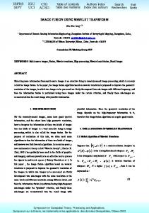
3. Modified complex Morlet wavelet Up to now, the traditional complex Morlet wavelet is commonly used for the CWT analysis, because it contains harmonic components similarly to the Fourier transform. The complex Morlet wavelet and its Fourier transform are given as follows (Kijeweski and Kareem, 2003): Complex Morlet wavelet N=5
Complex Morlet wavelet N=2 0.4 0.3
2
C
(1)
* x(t ) ,s (t )dt
(t )dt 0;
Wx ( , s )
0.3 real part imaginary part
fc=1, fb=2 Traditional
0.2 0.1
0.1
real part imaginary part
fc=1, fb=5 Modified
0 0
-0.1 -0.1
-0.2
-0.2
-0.3
-0.3 -0.4 -8
-6
-4
-2
0 2 t Complex Morlet wavelet N=2
4
6
8
0.4 0.3 0.2 0.1
-0.4 -8
-6
-4
-2 0 2 t Complex Morlet wavelet N=5
4
6
8
0.3 real part imaginary part
fc=2, fb=2 Modified
0.2 0.1
real part imaginary part
fc=2, fb=5 Modified
0 0 -0.1 -0.1 -0.2
-0.2
-0.3
-0.3 -0.4 -8
-6
-4
-2
0 t
2
4
6
8
-0.4 -8
-6
-4
-2
0 t
2
Figure 3. Modified Morlet wavelet with some parameters
4
6
8
Le et. al.
4 (t ) (2 ) 1/ 2 expi 2f c t exp t 2 / 2
ˆ ( sf ) ( 2 )
1 / 2
exp 2 sf f c
2
2
(5a) (5b)
where (t ),ˆ ( sf ) : complex Morlet wavelet and its Fourier transform coefficient. It is noted that here is only the central frequency as the traditional complex Morlet wavelet. Modified complex Morlet wavelet is used by Ladies and Gouttebroze, 2002; Yan et al., 2006 as follows:
time resolution and optimal frequency resolution. Kijewski and Kareem, 2003 discussed the time-frequency resolution for the wavelet transform using the traditional Morlet wavelet, also suggested for parameter selection. The time and frequency resolutions of the modified Morlet wavelet can be expressed as follows (Yan et al., 2006): f
1 2
(t ) (f b ) 0.5 exp( j 2f c t ) exp( t 2 / f b ) (6a) 2
2
ˆ ( sf ) exp( f b ( sf f c ) )
(7a) fb
fb 2
t
(6b)
(7b)
where fb: bandwidth parameter Investigations on the modified Morlet wavelet with some parameters (fc and fb) are shown in Figure 3.
where f , t : frequency resolution and time resolution of the modified Morlet wavelet. Here, relationship between the frequency and time resolutions is f t 1 4 considered as optimal product,
4. Time-frequency resolution analysis
normally
Analysis of the time-frequency resolution is inevitable for the close frequency identification and the high-mode parameter identification using the wavelet transform. Wavelet transform
f s
t st Frequency
Time
Figure 2. Time-frequency resolution plane Time-frequency resolution plane of the wavelet transform is shown in Figure 2, in which high frequency resolution and low time resolution are used for low frequency band, and inversely. The Heisenberg’s uncertainty principle revealed us that it is impossible to simultaneously obtain optimal
have
the
relationship
In the interrelation between the Fourier frequency and the wavelet central frequency, wavelet scale as shown in the Eq.(4), we have s f c f , one obtain the resolutions of time and frequency: f
Figure 2. Time-frequency resolution of wavelet transform
we
f t 1 4 .
f 2f c f b
(8a)
fc fb 2f
(8b)
Thus, one can adjust the wavelet central frequency fc and the bandwidth parameter fb to obtain the desired frequency resolution and the desired time one at analyzing frequency f.
5. Modal parameters estimation Consider a linear damped MDOF structure superimposed by N-modes, a response solution of the structure due to ambient external excitation as Gaussian distributed broad-band white noises can be expressed as follows:
5 N
X (t ) Ai exp(2 i f i t ) cos( 2f dit i ) X p (9) j 1
where N: number of combined modes; i: index of mode; Ai : amplitude of i-th mode; i : phase angle; f i , i : undamped frequency and damping ratio of i-th mode; f di f i 1 i2 : damped natural frequency; X p : perturbation due to noises and effect of
external excitation. There is no convincing study on the effect of the ambient loading on accuracy of the output-only system identification methods. It is noted that some authors (Ladies and Gouttebroze, 2002; Kijewski and Kareem, 2003 and so on) used the random decrement technique to eliminate the effect of external excitation and estimate impulse responses of structure. However, this technique as conditional correlation function and averaging processing can weaken high spectral components, but low energies in the signal. Normally, effect of perturbation due to noise and external excitation is eliminated. Substituting Eqs.(9) and (6) into Eq.(1), one can obtain the wavelet transform coefficient (Yan et al., 2006): WX ( , s )
s N Ai exp(2 i f i ) 2 i1
. exp( 2 f b ( sf i f c ) 2 ) exp( j ( 2f di i )) (10) Because the wavelet coefficient is localized at certain fixed scale s=si, thus only i-th mode associated with the wavelet scale s i dominantly contributes to Eq.(10), other modes can be negligible. Noting that from Eq.(4) we have si f c f i or si f i f c 0 , thus the term in Eq.(10) The wavelet exp( 2 f b ( sf i f c ) 2 ) 1. coefficient at scale si can be rewritten as SDOF system at i-th mode: WX ( , si )
si 2
Ai exp(2 i f i ) exp( j (2f di i ))
(11)
Substituting time t for translation , and expressing Eq.(11) in a form of the Hilbert transform’s analytic signal of instantaneous amplitude and instantaneous phase as follows: (12)
WX (t , si ) Bi (t ) exp( j i (t ))
where Bi (t ), i (t ) : instantaneous amplitude and phase, which are determined as: si Ai exp(2 i f i t ) 2 i (t ) 2f di t i
(13a)
Bi (t )
(13b)
Logarithmic expression of the instantaneous amplitude, then differentiating logarithmic amplitude, and differentiating the phase angle, one obtains: d ln Bi (t ) 2 i f i dt d i (t ) 2f i 1 i2 dt
(14a) (14b)
From Eqs.(14a) and (14b), the i-th natural frequency and the i-th damping ratio can be estimated as follows: 2
d ln Bi (t ) d i (t ) dt dt 1 d ln Bi (t ) i 2f i dt fi
1 2
2
(15a) (15b)
For estimating damping ratios from the wavelet logarithmic amplitude envelope, the linear fitting technique can be applied. Above-discussed wavelet transform-based procedure has been applied for estimating the natural frequencies and the damping ratios of ambient vibrated data of the structure.
6. Results and discussions Ambient vibration measurements have been carried out on a 5-storey steel structure at the test site of the Disaster Prevention Research Institute (DPRI), Kyoto University. Ambient data were recorded at all 5 floor levels and ground as reference, by tri-axial velocity sensors. Data were sampled on 5-minute
Le et. al.
6
2 1) DataFloor (Floor
-4
6
x 10
4 Amplitude(m)
2 0 -2 -4 -6 0
50
100
150 Time (s) Floor 1
1.74Hz
300
Mode 2
Mode 1
-8
10
5.35Hz
Mode 3 -10
8.84Hz
10
2
250
Power spectral density funtion
-6
10
PSD (m/s )
200
Mode 4 11.46Hz 13.68Hz
Mode 5 18.13Hz
-12
10
-14
10
-16
10
0
2
4
6
8
10 12 Frequency (Hz)
14
16
18
20
Figure 3. Data and its PSD coefficient (WTC) of the data on the frequency band 0÷20Hz and the time duration 50÷150seconds, with the central frequency fc=2 and the bandwidth parameter fb=20. As can be seen from Figure 4, there are only two frequency peaks observed at 1.73Hz and 5.34Hz, which correspond to two first modes. Frequencies of the high-order modes (the 3rd mode, 4th mode and 5th mode) can be estimated by this WCT. Reason is given here because single frequency
14 10 12 Frequency (Hz) 2 0
-16
10
-14
10
-12
10
10
-10
-8
10
10
P S D (m /s2 )
-6
1.74Hz
4
6
5.35Hz
8
8.84Hz
Floor 1
11.46Hz 13.68Hz
16
18
18.13Hz
20
records with 100Hz sampling rate (Kuroiwa and Iemura, 2007). Velocity outputs have been integrated to displacements for convenient use. Time series of the integrated displacement at first floor and its power spectral density functions (PSD) are presented in Figure 3. Combined with Finite Element Model (FEM) results, first five bending modes and associated natural frequencies can be identified. Figure 4 shows the wavelet transform
Figure 4. Wavelet transform coefficient (at fc=2, fb=20)
7 resolution has been applied to whole frequency band 0÷20Hz, which is good for low frequency analysis, but not appropriate to higher frequency bands. In order to identify the modal parameters of higher modes, it is proposed here techniques for frequency resolution adjustment as follows: (1) Bandwidth resolution adjustment: Analyzing frequency band is divided into several bandwidths, and one applies the Morlet wavelet with concrete parameters (fc, fb) to each frequency bandwidth. Here, there are bandwidths of 0÷20Hz such as 0÷5Hz, 5÷10Hz, 8÷12Hz, 12÷16Hz, and 16÷20Hz. (2) Broadband filtering: The data is broadband filtered into several bandwidths. This process remains desired frequency band for the wavelet transform coefficients, other undesired bands can be negligible. Next, the Morlet wavelet with adjusted frequency resolution applies to band-passed components. Here, the broadband filtered components of 0÷20Hz are 0÷3Hz, 3÷6Hz, 6÷12Hz, and 12÷24Hz.
(3) Narrowband filtering: Similar to the second technique, the signal is filtered not on broad bandwidths, but on narrow bandwidths, which are close to each natural frequency. This technique is much more localized around natural frequencies, but it requires prior information on these natural frequencies on the signal. Also, this technique eliminates effects of undesired frequencies on the wavelet coefficient analysis. Here, the data is filtered narrow bandwidths of 1÷3Hz; 4÷6Hz; 8÷10Hz; 13÷15Hz, and 17÷19Hz. Figure 5 shows the wavelet transform coefficients at four frequency bandwidths following the bandwidth resolution adjustment technique. The Morlet wavelet parameters (fc, fb) also are associated with the frequency bandwidths. Obviously, all the frequency peaks can be observed at each analyzing bandwidths, even close frequencies can be determined in the bandwidth of 12-16Hz. Broadband and narrowband components from the original data are shown in Figure 6. The frequency bandwidths also are indicated
Band 0÷5H, fc =2 fb=20
Band 5÷10Hz, fc=2 fb =50
Band 8÷12Hz, fc=3 f b=75
Band 12÷16Hz, fc=5 fb=50
Time (s)
Time (s)
Figure 5. Wavelet transform coefficient with bandwidth resolution adjustment
Le et. al.
8
Broadband filtering -4
x 10 2 0 -2 0x 10 -4 2
2
100
150
200
-4
Narrowband filtering Band 1-3Hz
Band 0-3Hz
50
x 10
0 -2 0x 10 -5 5
250
50
100
150
200
0
0
-2 0 -5 x 10 2 0 -2 0 -5 x 10 2 0 -2 0 -5 x 10 2 0 -2 0
50
100
150
200
250 Band 6-12Hz
50
100
150
200
250
A m p .(m /s)
A m p.(m/s)
250 Band 4-6Hz
Band 3-6Hz
-5 0x 10-6 5
50
100
150
200
250 Band 8-10Hz
0 -5 0x 10-6 2
50
100
150
200
Band 12-24Hz
250 Band 13-15Hz
0 50
100
150
200
250
-2 0x 10-6 1
50
100
150
200
Band 24-50Hz
250 Band 17-19Hz
0 50
100
150
200
250
-1 0
50
100
150
200
250
Time (s)
Time (s)
Figure 6. Broadband and narrowband filtering components Band 0÷3H, fc =2 fb=20
Band 6÷12Hz, fc =2 fb=20
Band 3÷6Hz, fc=2 fb=20
Band 12÷24Hz, fc=5 fb =50
Figure 7. Wavelet transform coefficient with bandwidth filtering in each filtered components. The wavelet transform coefficients of the broadband components and the narrowband ones, as shown in Figure 6 are presented in Figure 7 and Figure 8. As can be seen from the Figures 7 and 8, the natural frequencies, with application of the band-pass filtering are appeared more clearly and visibly than without filtering as in Figure 5. Although the close peak frequencies all can be observed in Figure 6 and Figure 7 at the natural frequency of the 4-th mode.
The wavelet transform coefficients are very clear observed when one applies the narrowband filtering (see Figure 8), especially, they are localized in the frequency domain but stretched in the time domain. This characteristic is convenient for estimating the damping ratios. Figure 9 shows the wavelet logarithmic amplitude envelopes of the wavelet transform coefficients of the narrowband components. The logarithmic decrements can
9
Narrowband at f1, fc=1 fb=20
Narrowband at f2, fc =2 fb=20
Narrowband at f3, fc =2 fb=20
Narrowband at f4 , fc=4 fb =50
Figure 8. Wavelet transform coefficient with narrowband filtering Wavelet logarithmicamplitude amplitude at f2=5.35Hz Wavelet logarithmic at f2
Wavelet logarithmic amplitude amplitude at f =1.73Hz Wavelet logarithmic at f1 1
-18
-8.6 y = - 0.033*x - 5.7
-18.2 Logarithmic amplitude
Logarithmic amplitude
-8.62
amplitude envelope linear fitting
envelope linear fitting
-8.64 -8.66 -8.68
-18.6
-18.8
-8.7 -8.72 87
-13
y = - 0.13*x - 8.6 -18.4
87.5
88
88.5 Time (s)
89
89.5
-19 72
90
Wavelet logarithmic at f3 Wavelet logarithmic amplitude amplitude at f =8.83Hz 3
-17
73
74
75 Time (s)
76
77
Wavelet logarithmic amplitude at f4 Wavelet logarithmic amplitude at f =13.64Hz 4
amplitude envelope linear fitting
amplitude envelope linear fitting
-13.1
78
Logarithmic amplitude
Logarithmic amplitude
-17.1 -13.2 -13.3 y = - 0.13*x - 2.2
-13.4 -13.5
-17.2
y = - 0.11*x - 8
-17.3
-17.4 -13.6 -13.7 83
83.5
84
84.5
85 Time (s)
85.5
86
86.5
87
-17.5 83
83.5
84
84.5
85 Time (s)
85.5
86
86.5
87
Figure 9. Damping estimation from wavelet logarithmic amplitude envelope be estimated via the linear least-square fitting technique as red lines shown in the same plots, the damping ratios then are determined. However, the questionable point here is that how is the time duration in the wavelet logarithmic amplitude envelopes selected for estimating the damping ratios.
There is no any discussion on this matter, but it is generally agreed that the selection of time duration much influences on accuracy and reliability of identified damping ratios. It argues that some following guidelines should be taken into consideration for damping estimation:
Le et. al.
10 (1) Time duration should start around clear and maximum peak of wavelet transform coefficient. (2) Short localized time duration should be preferable. Table 1. Identified natural frequencies (Hz) PSD WT(1) WT(2) WT(3)
Mode1
Mode2
Mode3
Mode4
Mode5
1.74 1.74 1.73 1.73
5.35 5.32 5.34 5.35
8.84 8.81 8.82 8.83
13.68 13.64 13.59 13.64
18.13 18.07 18 18.04
Table 2. Identified damping ratios (%) Mode1
Mode2
Mode3
Mode4
Mode5
0.52 2.07 2.07 1.75 2.22 Note: WT(1), (2), (3) corresponding to frequency resolution techniques as (1) bandwidth adjustment; (2) broadband filtering; and (3) narrowband filtering
WT(3)
Results of the natural frequencies and damping ratios extracted from mentioned three techniques are listing this Table 1. There is good agreement observed for the identified natural frequencies between the techniques.
7. Conclusion Output system identification of ambient data using the wavelet transform has been presented in the paper. Modified Morlet wavelet is more adaptive and appropriate to treat with sophisticated time-frequency resolution analysis. Three frequency resolution techniques have been proposed to estimate the modal parameters of the highorder modes and the close frequency problem. Identified natural frequencies from three techniques are good agreement. However, further investigations on selection of time duration in the wavelet logarithmic amplitude envelopes are required for more reliability and accuracy of the damping estimation.
Acknowledgement. This study was funded by the Ministry of Education, Culture, Sport, Science and Technology (MEXT), Japan through the Global Center of Excellence (Global COE) Program, 2008-2012. Real data were permitted for use by Dr.Kuroiwa at Structural Dynamics Laboratory, Kyoto University for which the first author would express the special thank.
References Daubechies, I. (1992). Ten lectures on wavelets. CBMS-NSF. Kijewski, T.L., and Kareem, A. (2003). Wavelet transforms for system identification: considerations for civil engineering applications. Journal of Computer-aided Civil and Infrastructure Engineering, 18, pp.341-357. Kuroiwa, T., and Iemura, H. (2007). Comparison of modal identification of output-only systems with simultaneous and non simultaneous monitoring. Proc. the World Forum on Smart Materials an Smart Structures Technology (SMSST07), Chongqing & Nanjing, China. Ladies, J., and Gouttebroze, S. (2002). Identificationof modal parameters using wavelet transform. Int’l Journal of Mechanical Science, 44, pp. 2263-2283. Meo, M., Zumpano, G., Meng, X., Cosser, E., Roberts, G., and Dodson, A. (2006). Measurement of dynamic properties of a medium span suspension bridge by using the wavelet transform. Mechanical Systems and Signal Processing, 20, pp. 1112-1133. Slavic, J., Simonovski, I., and Boltezar, M. (2003). Damping identification using a continuous wavelet transform: application to real data. Journal of Sound and Vibration, 262, pp. 291-307. Staszewski, W. J. (1997). Identification of damping in MDOF systems using time-scale decomposition. Journal of Sound and Vibration, 203, 2, pp. 283-305. Yan, B.F., Miyamoto, A., and Bruhwiler, E. (2006). Wavelet transform-based modal parameter identification considering uncertainty. Journal of Sound and Vibration, 291, pp. 285301.