Observations of a unique type of ULF waves by low-latitude Space Technology 5 satellites
G. Le1, P. J. Chi2, R. J. Strangeway2, and J. A. Slavin1 (1) Heliophysics Science Division, NASA Goddard Space Flight Center, Greenbelt, MD 20771 (
[email protected];
[email protected]) (2) Institute of Geophysics and Planetary Physics, University of California, Los Angeles, CA 90095 (
[email protected];
[email protected])
to be submitted to J. Geophys. Res. – Space Physics Correspondence should be sent to: Guan Le Mail Code 674 NASA Goddard Space Flight Center Greenbelt, MD 20771, USA Phone: (301)286-1087 Fax: (301)286-1648 Email:
[email protected]
1
Abstract We report a unique type of ULF waves observed by low-altitude Space Technology 5 (ST-5) constellation mission. ST-5 is a three micro-satellite constellation deployed into a 300 x 4500 km, dawn–dusk, and sun synchronous polar orbit with 105.6° inclination angle. Due to the Earth’s rotation and the dipole tilt effect, the spacecraft’s dawn-dusk orbit track can reach as low as subauroral latitudes during the course of a day. Whenever the spacecraft traverse across the dayside closed field line region at subauroral latitudes, they frequently observe strong transverse oscillations at 30-200 mHz, or in the Pc 2-3 frequency range. These Pc 2-3 waves appear as wave packets with durations in the order of 5-10 minutes. As the maximum separations of the ST-5 spacecraft are in the order of 10 minutes, the three ST-5 satellites often observe very similar wave packets, implying these wave oscillations occur in a localized region. The coordinated ground-based magnetic observations at the spacecraft footprints, however, do not see waves in the Pc 2-3 band; instead, the waves appear to be the common Pc 4-5 waves associated with field line resonances. We suggest that this unique Pc 2-3 waves seen by ST-5 are in fact the Doppler-shifted Pc 4-5 waves as a result of rapid traverse of the spacecraft across the resonant field lines azimuthally at low altitudes. The observations with the unique spacecraft dawn-disk orbits at proper altitudes and magnetic latitudes reveal the azimuthal characteristics of field-aligned resonances.
2
1. Introduction The magnetosphere can undergo various types of oscillations in the Ultra-low-frequency (ULF) band (i.e., frequencies ranging from ~ 1 mHz to 1 Hz). These magnetospheric waves play significant roles in mediating processes in solar wind-magnetosphere-ionosphere coupling, including transporting the solar wind stresses and energy through the magnetosphere, energizing particles in the inner magnetosphere, and causing particle precipitations into the ionosphere. These waves have been used to diagnose and understand the state of the magnetosphere by analyzing their frequencies and travel times [see a recent monograph by Takahashi et al., 2006 and the references therein]. For example, the Pc 1 (0.2-5 s) waves can interact with the cyclotron motion of ions and cause their energization and pitch angle scattering in the inner magnetosphere [see a review by Kangas et al., 1998]. The Pi2 (40-150 s) waves are frequently observed at substorm onsets [e.g., Olson, 1999], and have recently been used to estimate the time and location of substorm initiation in the magnetotail [Chi et al., 2009]. The Pc 3-5 (10-600 s) waves are ubiquitous in the magnetosphere, and these long-period magnetohydrodynamic (MHD) waves are often related to magnetospheric field line and cavity resonances [Tamao, 1965; Kivelson and Southwood, 1985; Chen and Hasegawa, 1988]. In particular, observations of field line resonance by ground magnetometers have been used to monitor the state of the magnetosphere during storm times [e.g., Chi et al., 2000; Chi et al., 2005]. Among the observations of various types of ULF waves, those in the Pc2 (5-10 s) band and the high-frequency portion of the Pc3 band have been relatively rare. Pc2 waves were initially thought to be a nightside phenomenon [e.g., Jacobs, 1964], but the concept became 3
questionable when ground observations showed that the Pc2 distribution had a peak at noon [Kangas et al., 1998]. Most studies on Pc2 waves were reported together with Pc1 waves as the frequency of the electromagnetic ion cyclotron (EMIC) waves – which commonly resides in the Pc1 band – can drop to Pc2 and even Pc3 bands when oxygen ions are present [e.g., Fraser et al., 1992]. These EMIC waves in the Pc2 band have been observed both in space and on the ground, more likely in the afternoon sector [Fraser, 1968]. They are generated by the ion cyclotron instability in the equatorial region and can propagate to the ionosphere and the ground [e.g., Cornwall et al., 1970; Morley et al., 2009]. Unstructured Pc1-2 waves can also be found poleward of the dayside cusp, possibly with a source location in the high-altitude plasma mantle [Engebretson et al., 2005], and within the high-altitude (5-9 RE) polar cusp [Le et al., 2001]. Like the Pc3-4 waves, the Pc2 waves can also occur as a result of the upstream waves in the foreshock region [Troitskaya et al., 1971] during intervals with an unusually strong interplanetary magnetic field (IMF). In this scenario a low IMF cone angle is a preferable condition for the wave occurrence in the magnetopshere, and the waves are dominant in the dayside region. Most of the reported in situ observations of ULF waves by satellites are in the magnetosphere at high altitudes; and wave observations at topside ionosphere are very limited. Due to their rapid motion, satellites in the topside ionosphere are usually considered to be able to adequately observe waves only in the high-ULF band. Magsat observed Pc1 pulsations in the ionospheric F region, which are stronger than their ground counterpart by two order of magnitude [Iyemori and Hayashi, 1989]. Erlandson and Anderson [1996] surveyed the Pc1 waves observed by the Dynamic Explorer 2 (DE-2) satellite in the ionosphere and concluded that they occurred most frequently at frequencies between 0.4 and 2.0 Hz, in the dawn and noon 4
sectors, and within 50° to 62° invariant latitude range. Using observations from Space Technology 5 (ST-5) satellites, Engebretson et al. [2008] found that Pc1 wave activities were not only localized in L-value but could appear and disappear on the time scales of ~10 s to 10 min. In recent years the low-altitude observations by the CHAMP satellite (h = 350-450 km) also motivated and enabled several studies examining the waves at lower ULF frequencies. Sutcliffe and Lühr [2003] reported that the compressional and poloridal components of the Pi2 pulsations above the ionosphere were well correlated with the H-component of Pi2 on the ground. In the Pc3 frequency band Heilig et al. [2007] and Ndiitwani and Sutcliffe [2009] found that the compressional power was unexpectedly large at low altitudes and that the source energy came from the upstream waves. Pilipenko et al. [2008] provided analytical and numerical models to demonstrate how this compressional wave component could result in magnetic signatures on the ground. This paper reports a new type of Pc 2-3 waves observed by Space Technology 5 (ST-5) constellation, which appears to be unique and has never been reported before to our knowledge. ST-5 is a three-satellite constellation mission deployed to a dawn-dusk, ~ 300 x 4500 km sunsynchronous polar orbit from March to June, 2006 for technology validations [Slavin et al., 2008]. The three ST-5 satellites, each carried a research grade fluxgate magnetometer, observed strong transverse oscillations at 30-200 mHz (spanning Pc 2 and high-Pc 3 bands) as the satellites quickly traversed longitudinally across the closed field lines in the dayside. A careful examination of the waves seen by all three ST-5 satellites as well as neighboring ground magnetometer stations leads to a conclusion that these unique Pc 2-3 waves are in fact Dopplershifted Pc 4-5 magnetospheric waves in the Earth frame as a result of the rapid traverse of spacecraft at low altitudes. Estimated by the observed frequency and the satellite trajectory, the 5
azimuthal wave numbers (m) of these magnetospheric pulsations are in the order of 100. The frequent occurrence of high m waves is an unexpected result because the observations of such waves were only sparsely reported in the past. Our results strongly imply that these high-m waves are in fact a common phenomenon in the dayside magnetosphere, and they can be observed only when the satellites are in the right locations and orbits. We will present the detailed ST-5 observations in Section 2, coordinated ground-based observations for one of the event in Section 3, the discussions in Section 4, and finally the conclusions in Section 5.
2. ST-5 Observations 2.1. Observation Overview The ST-5 orbit is sun-synchronized in the dawn-dusk meridian plane and the three satellites are in a string-of-pearl configuration. The orbit period is ~ 136 minutes and the inclination angle of the polar orbit is 105.6°. Due to the Earth’s rotation and the dipole tilt effect, the spacecraft’s dawn-dusk orbit tracks over the polar cap span a large latitudinal range during the course of a day, reaching as low as subauroral latitudes. Whenever the spacecraft traverse across the dayside region at subauroral latitudes, they frequently record strong oscillations in 30200 mHz band, or in Pc2-3 frequencies, in the magnetic field components. We first present a detailed example to illustrate where the waves are observed and how they appear in ST-5 data. Figures 1-2 presents an overview of the ST-5 observations on April 8, 2006 from one of the three spacecraft. The ST-5 spacecraft with ~ 136 min orbital period go around the Earth about 10 times a day. Figure 1 shows 8 spacecraft orbit tracks over the northern polar cap during 6
this day. The orbit tracks are mapped to their ionospheric footprints along the magnetic field lines and displayed in the Solar Magnetic (SM) coordinate system. In Figure 1, the Sun is to the right, the dusk is vertically up, and the circles are for the constant magnetic latitudes. The orbit tracks of the spacecraft are in the dayside during the northern polar cap passes, and the spacecraft move from dusk to dawn. The spacecraft cross the dayside ionosphere at various latitudes during the course of a day. At local noon, the geomagnetic latitude of the footprint ranges from ~ 83° in the polar cap down to ~ 63° in the dayside subauroral region. We label the orbits with numbers 1 to 8 based on their subsolar latitudes from high to low. The corresponding magnetic field measurements for these orbits are shown in Figure 2. The data for the four higher latitude orbits are in panels (1)-(4), all of which are above the auroral zone at local noon. The magnetic field observations for these higher latitude orbits exhibit those of typical field-aligned current signatures [Le et al., 2009, 2010]. In panels (1), (2) and (4), it is clear that the spacecraft crosses the auroral zone twice, and thus the magnetic field perturbations associated with large scale field-aligned currents are evident in both morning and afternoon side separating by polar cap magnetic field. In panel (3), the field-aligned current signatures appear from near dawn to past local noon, indicating the spacecraft skims the auroral zone in this pass. The magnetic field observations for the four lower-latitude passes in panels (5)-(8) are markedly different from those at higher latitudes (Please note different vertical scales in the top and bottom panels). First of all, the signatures of large-scale field-aligned currents are absent, indicating the spacecraft trajectories are all equatorward from the auroral zone and the polar cusp, i.e., in subauroral latitudes. The low-frequency variations in the magnetic field components 7
as well as the magnetic field strength are the signatures of Earth’s crustal magnetic fields [Purucker et al., 2007]. They are mainly visible by the ST-5 spacecraft near the orbit perigee at altitudes below ~ 600 km. Secondly, it is evident that waves appear in the magnetic field data. The wave signatures are seen only in the magnetic field components, but not in the magnetic field strength. Thus, the wave oscillation fields are in the directions transverse to the background magnetic field. The frequencies of these transverse waves are in the range of ~ 30-200 mHz, or in the Pc2-3 band as seen by the spacecraft. These Pc2-3 waves appear as wave packets with durations in the order of 1-10 minutes. By examining the data from the entire ST-5 mission, we find that these occurrence characteristics are always true. This type of waves are only observed at subauroral latitudes, or below ~ 75° magnetic latitudes.
2.2. Statistical Occurrence of the Waves Figure 3 shows the spatial occurrence of the waves based on the entire three-month ST-5 mission. In Figure 3(a), ST-5 spacecraft positions are mapped to the ionospheric footprints along the magnetic field lines in the northern hemisphere. The black dots represent the center locations of one-minute ST-5 orbit segments. The red dots superposed on top of black dots are for times when the Pc2-3 waves are observed, again in one-minute segments. Figure 3(b) shows the same orbits but mapped to the equatorial plane along the magnetic field lines. The statistical occurrence pattern shows that these waves are a phenomenon of dayside subauroral latitudes and occur in the magnetosphere on closed field lines. The vast majority of the wave events are observed within ~ 3 hours from the local noon and below ~ 75° magnetic latitudes in ionosphere. When mapped to the equatorial magnetosphere, it is clear these waves are all on dayside closed 8
field lines, with the majority located within L~9. Since the lowest magnetic latitudes at ST-5 ionospheric footprints are ~ 63° at local noon, it is very likely that the waves can also been seen below ~ 63° magnetic latitudes and below L~7 in the magnetosphere. We have also examined how frequently the waves occur in the magnetosphere during the ST-5 period. During the 3-month mission the magnetic field data are available for 89 days, from March 27 to June 23, 2006. In 78 days out of the 89 days, we have observed the waves in at least one of the passages across the subauroral region. We can determine the overall occurrence rate of the waves in the dayside subauroral region using then entire ST-5 data set (regardless of solar wind/magnetospheric conditions). In doing so, we divide the dayside ionosphere into grids with 1-hour local time bins and 5° latitude bins, as shown in Figure 4. Within each grid, we determine the total amount of time the spacecraft spend inside and the total amount of time when waves are present, i.e., the total number of black dots and red dots in each grid, respectively. The wave occurrence rate is the ratio of the number of red dots to the number of black dots in each grid and its spatial distribution is shown in Figure 4. The maximum occurrence is in the dayside subsolar region. In the region below 75° magnetic latitude and within 0900 and 1500 local time, the wave occurrence rate is greater than 20%. The peak of the wave occurrence reaches more than 30% in the subauroral region near the local noon between 65° and 70° in magnetic latitudes.
2.3. Simultaneous Multi-point Observations by Three Spacecraft The three spacecraft of the ST-5 constellation provide simultaneous multipoint measurements of the waves and enable us to examine the wave properties. We use one of the 9
wave intervals presented in Figure 2 to demonstrate what we can learn from the multi-point observations. Figure 5 shows an overview of the wave event on April 8, 2006. The left panel is the orbit tracks of the three spacecraft that are mapped to their ionospheric footprints. The three ST-5 spacecraft are named SC094, SC155 and SC224, and their trajectories are color coded in black, red and blue, respectively. The tick marks for each trajectory are separately by 5 minutes. During this time period, the spacecraft move azimuthally from dusk to dawn in the region equatorward from the auroral zone. The most poleward location of the orbit track is ~ 75° geomagnetic latitude at the local noon. In the string-of-pearl configuration, the mid-spacecraft SC094 (black) and the trailing spacecraft SC224 (blue) are close together and have a large separation from the leading spacecraft SC155 (red). The orbital separation between the leading spacecraft and mid-spacecraft is about 8 minutes, and between the mid-spacecraft and trailing spacecraft less than 1 minute. The right panel of Figure 5 shows an overview of ST5 magnetic field measurements for this pass, including the three components of the magnetic field residual vector (data with the internal IGRF model magnetic field removed) in the solar magnetic (SM) coordinate system, as well as the residual of the magnetic field strength. The data from the three spacecraft are color coded corresponding to those of the spacecraft orbits in the left panel, but the labels for the spacecraft positions (altitudes, magnetic latitudes and magnetic local times) on the bottom of the panel are for mid-spacecraft SC094 only. The magnetic field data shown in Figure 5 all have a time resolution of 1 s, which are spin-averaged data with overlapped averaging windows. The spin periods are about 3 s and are slightly different for the three spacecraft.
10
All the three ST-5 spacecraft observe the wave packets in the dayside near the local noon. The waves are nearly monochromatic, and the wave packets last about 5 minutes in the data. The wave oscillations are completely confined in the three components of the magnetic field; no trace of the waves can be seen in the magnetic field strength. Thus, these waves are purely transverse waves. The peak-to-peak amplitudes of the waves are in the range of 10 - 40 nT. We note that the Earth’s internal magnetic field as represented by the IGRF model is over 40,000 nT in the location where the waves are observed. In order to resolve the wave structures in such a strong background magnetic field, the magnetometers need to be highly sensitive and accurate. We speculate that this is probably one of the reasons the same kind of waves have never been reported before in spacecraft data even through they occur so frequently in the ST-5 data. We apply a high-pass filter to the data and then perform the minimum variance analysis [Sonnerup and Cahill, 1967] to the filtered data. Figure 6 shows the high-pass filtered data in the Minimum Variance Coordinates. Since the spacecraft motion is mainly in the longitudinal direction, we display the high-pass filtered magnetic field as a function of the magnetic local time in Figure 6, which also provides information on the wave packets’ spatial extents and their temporal variations. The three components of the magnetic field (δBi, δBj, δBk) correspond to the directions of minimum, intermediate, and maximum variances, respectively. The minimum variance direction i is along the background magnetic field direction since the wave is purely transverse wave. From Figure 6, we can make following observations: (1)
The wave amplitude in the maximum variance direction δBk is much larger than that in the intermediate variance direction δBj, so the wave polarization is
11
highly elliptical or nearly linear in the plane transverse to the background magnetic field. (2)
All the three spacecraft observed the wave packets in the same local time region from 13 to 15 MLT, even through there is a ~ 8 minutes orbital time lag from the leading spacecraft and the mid- and trailing spacecraft. Thus, the wave packet stays in the same spatial region during this 8 minutes time interval.
(3)
The wave forms in δBk show very small phase shifts within the wave packets among the three spacecraft. We can use the data to estimate the azimuthal phase velocity of the wave. The orbital time lag between the leading and midspacecraft is ~ 8 minutes. The phase shift of the wave forms observed by them is in the order of 5 minutes in local time, or ~ 1° in longitude. Thus the longitudinal phase velocity of the wave is in the order of ~ 0.1° per minute. On the other hand, during the time interval of ~ 5-minute duration of the wave packet, the spacecraft have moved from ~ 15 MLT to ~ 13 MLT, spanning about 30° in longitudes. So the longitudinal velocity of the spacecraft is ~ 6° per minute, much greater than the wave longitudinal velocity. Thus, the waves can be treated as stationary in the longitudinal direction comparing with the fast motion of the spacecraft.
Figure 7 further supports the observation (1) above. It shows the wave magnetic field vectors along the spacecraft orbit track for the mid-spacecraft only. The left panel is the projection on the XY plane as viewed from the north, and the right panel the projection in the YZ 12
plane as viewed from the Sun. They show that the wave magnetic fields are highly elliptically polarized. The polarization of the strongest waves is mainly in the radial direction, or roughly in the magnetic meridional plane. Figures 8-10 shows another example of the wave on May 7, 2006. Figure 8 shows the spacecraft footprint trajectory across the dayside subauroral region from dusk to dawn (left panel) and the corresponding magnetic field data (right panel). The tick marks on each trajectory are separated by 5 minutes. For this event, the orbital delay from the leading spacecraft to the mid-spacecraft is about 3 minutes, and from mid-spacecraft to trailing spacecraft about 1 minute. All three spacecraft observe the similar Pc2-3 waves in the right panel. Figure 9 has the same format as in Figure 6. Here the Pc2-3 waves occur in the same local time region from ~ 8 to 15 MLT at the three spacecraft. Similar to the previous case, the waves packet remains in the same local time region as the three spacecraft cross the region successively with time lags up to ~ 4 minutes. The three spacecraft observe very small longitudinal phase velocity of the wave comparing with the longitudinal velocity of the spacecraft. Figure 10 shows the wave magnetic field vectors along the spacecraft obit track, in the same format as in Figure 7. It shows again that the waves are nearly linearly polarized. The polarization of the strongest wave portion is largely in the radial direction, or in the magnetic meridional plane. The two wave examples above present common features and properties of the waves observed by ST-5. As the maximum orbital time lag in the order of 10 minutes, the waves appear to stay in the same local time region in time scales up to ~ 10 minutes as seen successively by the three spacecraft.
13
3. Ground-based Observations Ground-based magnetometer array has long been used to monitor the dynamics of the Earth’s magnetosphere, such as the excitation of ULF pulsations, as many of these waves in the magnetosphere can be detected on the surface of the Earth. Ground-based magnetic field data from a large array are very useful in the study of the spatial patterns and propagation of the waves. In particular, by comparing the wave phases recorded by closely spaced ground stations in the north-south direction one can readily identify field-line resonance (FLR) signatures even when the wave power is very weak in the power spectrum [e.g., Chi and Russell, 1998]. Here, we use simultaneous ground-based magnetometer data during the ST-5 wave occurrence to examine the ULF waves on the ground and the state of magnetospheric oscillations, in particular the expected FLR wave occurrence and frequencies in the dayside magnetosphere. For the ST-5 wave event presented in Figure 8 (May 7, 2006), there are simultaneous ground-based magnetic field data available from CARISMA ground magnetometer array [Mann et al., 2008] at locations near the ST-5 spacecraft ground tracks. Figure 11 shows the map of ST5 footprints and locations of selected ground magnetometer stations near the spacecraft ionospheric footprints for the May 7, 2006 wave event. The grids of dotted thin lines are for constant geomagnetic latitudes and longitudes. Moving from southeast to northwest, the footprints of ST-5 spacecraft pass over the Island Lake (ISLL), Rabbit Lake (RABB), and Contwoyto (CONT) stations. The wave occurrence at the ST-5 mid-spacecraft (black trace and tick marks) is from ~ 2211 to 2218 UT, corresponding to magnetic latitudes between 68° and 73°. Three stations to the east, Rankin (RANK), Fort Churchill (FCHU), and Gillam (GILL), are also located in the same latitudinal range of 68° to 73° where the ST-5 observed Pc2-3 waves. 14
These three stations, together with ISLL and several McMAC stations at lower latitudes (open squares), are approximately along the 330° magnetic meridian, and their data can be used for identifying FLR frequencies as described later in this Section. Figure 12 is a stack plot of the geographic north components of the magnetic field data observed by the 6 CARISMA ground stations from 2200 to 2225 UT on May 7, 2006, which covers the entire ST-5 wave interval in Figure 8. The top four traces are for the stations at 330° meridional chain and ordered according to the magnetic latitude of the station. The bottom two traces are for the two stations located to the west of the 330° meridional chain and under ST-5 orbit tracks. The baseline for each trace is arbitrary; and the vertical scale only represents the amplitude of the magnetic field variation. As evident in Figure 12, the dominant wave activities observed by these ground stations have frequencies in the Pc5 band, approximately 4-6 mHz. These Pc5 waves on the ground do not appear in the ST-5 data; and the ST-5 Pc2-3 waves are not seen in the ground-based data either. The differences of the wave characteristics at ST-5 and on the ground are evident in the wave power spectra shown in Figure 13. On the top are three power spectra for the X component of the magnetic field observed by the three ST-5 spacecraft; the spectra of the six CRISMA stations are plotted below. At the ST-5 spacecraft, enhanced wave power was observed at frequencies ranging from 8 mHz to 0.2 Hz. On the ground, the spectral peaks occur in Pc5 band, as indicated by arrows. These arrows also show the pattern of latitudinal variations of the spectral peaks. The observed Pc5 wave peak frequencies are the lowest at high-latitude stations RANK, FCFU and CONT. In comparison the Pc5 wave frequency at the lower-latitude station ISLL is clearly higher. The latitudinal dependence of the Pc5 wave frequency is indicative of an FLR origin of these waves [Singer and Kivelson, 1979; 15
Waters et al., 1991], and the evidence of FLRs will be presented later by using the cross-phase spectrograms between the observations by a closely spaced pairs of magnetometers. In the frequency range of the Pc2-3 waves observed by ST-5, the ground-based observations do not show any clear evidence of enhanced power in the same Pc2-3 frequency band – except a clear spectral peak at about 30 mHz at ISLL (Figure 13). Many studies have developed the so-called gradient analysis techniques using groundbased magnetometer data from a closely spaced station pair to elucidate the nature of magnetospheric ULF waves [e.g., Baransky et al., 1985; Waters et al., 1993]. For example, in the cross-phase spectrograms between a pair of stations separated in latitudes, FLR signatures can be readily recognized by large phase differences between the two stations even through the FLR signals are very weak in power. We now apply the cross-phase technique to a pair of latitudinally separated ground stations located very close to the ST-5 footprint, GILL and ISLL. Figure 14 is the cross-phase spectrogram showing the phase differences between the northward components of GILL and ISLL data. The two stations are separated by 2.5° in latitude, a spacing suitable for such gradient analysis. The time interval of the spectrogram in Figure 14 covers essentially the entire daytime hours of May 7, 2006, as the local time of the two stations is approximately UT−6.5 hours. In cross-phase spectrograms, FLR signatures can be recognized by large phase differences between the two stations. During 2145-2245 UT, the time interval for the wave spectra shown in Figure 12, large phase differences were found for frequencies at ~6 mHz and ~28 mHz. These FLR signatures also appeared at similar frequencies earlier for most daytime hours of the day. An FLR signature is also shown at ~16 mHz during 1600-1700 UT. The cross-phase spectrogram 16
implies that the enhanced wave power at ~30 mHz seen by station ISLL is the third harmonic of the FLR (and we denote it as f3 in Figure 12). This third harmonic FLR frequency is location dependent, and the higher latitude stations RABB and CONT do not see it. Therefore we do not consider that the spectral peak at ~30 mHz observed at ISLL is related to the Pc2-3 waves observed by ST-5. These cross-phase spectrogram observations indicate that fundamental mode of FLRs is present in the entire dayside region at the ST-5 footprints during the Pc2-3 wave occurrence although the same Pc2-3 waves are absent in the ground-based observations. With the observations along the 330o magnetic meridian, including those from the McMAC stations Glyndon (GLYN), Bennington (BENN), Americus (AMER), and Purcell (PCEL), we can confirm the latitudinal dependence of FLR frequencies discussed earlier. Using the same cross-phase technique as in Figure 13, we identify the FLR frequencies for other pairs of adjacent stations. The fundamental mode frequencies as a function of magnetic latitudes are summarized in Figure 15. For each station pair the data point is plotted at the latitude midway between the two stations.
As expected, the fundamental mode frequency increases with
decreasing latitude. The four data points on the right above 60° magnetic latitude form a linear line; whereas the three data points on the left below 60° seem to follow a linear line with a different slope. This change of slope is a typical result that have been seen in FLR frequencies identified using ground magnetometers, and in this case it indicates a plasmapause located somewhere between 53° and 60° magnetic latitude.
4. Discussions
17
In this section, we first discuss why the ST-5 and ground-based observations lead us to believe that the Pc2-3 waves at ST-5 are related to the Pc5 waves on the ground. We have demonstrated in the May 7, 2006 event that the Pc5 waves on the ground are signatures of FLRs in the magnetosphere. The Pc2-3 waves at ST-5 are most probably related to the azimuthal structure of the high-m number counterpart of FLR oscillations, which are only detectable in space. We then discuss what we know about the properties of high-m number ULF waves how our observations would help in understanding high-m number ULF waves and associated particle dynamics in the inner magnetosphere. 4.1. Origin of the Pc 2-3 waves observed by ST-5 To assist the discussions about the origin of the Pc2-3 waves, we summarize the key observations by the ST-5 spacecraft and the concurrent ground observations: (1) The Pc2-3 waves are observed by the orbiting ST-5 satellites in the topside ionosphere. (2) The Pc2-3 waves at ST-5 occur at dayside subauroral altitudes below ~ 75° magnetic latitudes and map to the region of closed field lines in the dayside magnetosphere. (3) The ST-5 satellites observe the Pc2-3 waves frequently regardless of solar wind conditions. (4) The dominant wave component is in the poloidal mode with polarizations in inward/outward radial directions.
18
(5) The same Pc2-3 waves are not observed on the ground stations located near the footprints of ST-5 trajectories. Instead, ground-based observations reveal typical Pc5 field line resonances in dayside hours These peculiar features of the Pc2-3 waves at ST-5 indicate that these waves are unlikely to be the same Pc2 waves reported in literature.
Since observed only in the dayside
magnetosphere, these waves are also unlikely to be associated with any phenomenon in the nightside. Their occurrence is at latitudes much lower than the cusp and in the region of closed field lines, and therefore the waves are not the same as the unstructured Pc1-2 waves within or poleward of the dayside cusp as reported by Le et al. [2001] and by Engebretson et al. [2005]. The Pc 2-3 waves are also different from other types of ULF waves observed by ST-5 or other low-altitude satellites in the Pc1, Pi2, and Pc3 frequency bands [e.g., Erlandson and Anderson, 1996; Engebretson et al., 2008; Heilig et al., 2007; Ndiitwani and Sutcliffe, 2009]. One may also speculate the possibility that the ST-5 Pc2-3 waves are the EMIC waves induced by the ion cyclotron instability near the equatorial region. Although the association with the EMIC waves requires further investigation, we find that the statistical occurrence of the observed ST-5 Pc2-3 waves is not consistent with that of the EMIC waves. Statistically the EMIC waves occur at all local times [e.g., Anderson et al., 1992]. Geomagnetic storms are well known to populate the ring current region with energetic ions, leading to enhanced occurrence of the EMIC waves [e.g., Erlandson and Anderson, 1996]. In contrast, the Pc2-3 waves at ST-5 occur mainly in the dayside magnetosphere at subauroral latitudes, and these waves can be seen in the region approximately 30% of the time regardless of the solar wind and geomagnetic conditions. As a matter of fact, the entire 90 days for the ST-5 mission occur in a period of quiet 19
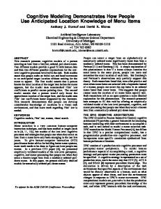
and moderate geomagnetic activities. In addition, it would be difficult to understand, when ST-5 satellites see the Pc2-3 waves in the ionosphere at altitudes of a few hundred kilometers, why ground stations right underneath the satellites do not detect the same type of waves. Based on the above considerations we believe that the Pc2-3 waves observed by ST-5 are unlikely to be the EMIC waves. In the May 7, 2006 event presented above, the ground-based observations show that the observed ground Pc5 waves are caused by FLRs and they are present in dayside hours at the same latitudes as the ST-5 footprints. Therefore, the ST-5 satellites would pass through the region of FLR when they move in the ionosphere above these ground stations. If the FLR has a finite azimuthal wavelength, however, the rapid motion of the ST-5 satellites in the longitudinal direction means that the wave frequency at the spacecraft would be related to the azimuthal wave number of FLRs due to Dopper-shift. Figure 16 is a schematic of FLR wave field and its azimuthal structure, in which the wave field has a low frequency in the Earth frame and a small azimuthal wavelength (or a large azimuthal wave number). When a spacecraft travels across the resonant field lines with a high azimuthal speed, the azimuthal structures of field lines would appear as a higher frequency waves due to the Doppler effect. The wave frequency at the spacecraft depends on the FLR azimuthal wave number as well as the spacecraft azimuthal speed. We can estimate the FLR azimuthal wave number based on the observed wave frequency at the spacecraft. Considering the scenario shown in Figure 16, we can make a rough estimate of the azimuthal wave number based on the ST-5 observations in the 7 May 2006 event. If we focus on the condition where the spacecraft travels in the azimuthal direction, the Doppler effect 20
gives the following relationship between the wave frequency observed by the spacecraft and that in the stationary (Earth) frame:
(1)
where ω and ω’ are wave frequency in the Earth frame and spacecraft frame, respectively, ky FLR azimuthal wave vector, m FLR azimuthal wave number, v longitudinal speed of the spacecraft, and dϕ/dt angular velocity of the spacecraft. At the magnetic latitudes where ST-5 observed Pc2-3 waves, the typical fundamental mode frequency of FLR is a few mHz, which is considerably smaller than the Pc2-3 frequencies observed by ST-5. As ω 15 have been reported occasionally in case studies using either satellite or HF radar data [Fenrich and Samson, 1997; Wright and Yeoman, 1999; Baddeley et al., 2005; Eriksson et al., 2006; Schafer et al., 2007; Yeoman et al., 2008; Yang et al., 2010]. Radar Observations show that the high-m number waves co-exist with the low-m number and they share many common features [Fenrich and Samson, 1997; Wright and Yeoman, 1999]. Both the high-m and low-m resonant waves occur at 22
the similar discrete frequencies, in the similar local time range and L-shells. Satellite observations in space show that high-m number waves exhibit characteristics of fundamental poloidal waves, consistent with the theoretical prediction that the high-m number oscillations are dominant by the poloidal mode [Southwood and Kivelson, 1982]. The ST-5 observations presented in this paper are in general agreement with this key feature of high-m number waves. Several studies have determined the m-value of high-m number waves bases on phase differences among simultaneous measurements from multiple Cluster spacecraft. Eriksson et al. [2006] reported a case of high-m waves in the dayside magnetosphere with m ~ 130. Schäfer et al. [2007] identified a case of 16 mHz pulsations with m ~ 30. Yang et al. [2010] reported a stormtime high-m number wave with m ~ 22 ± 3. Since the phase-difference technique requires multiple spacecraft separating in the azimuthal direction to determine the m-value, the observational cases in the magnetosphere are very limited and there is a lack of statistical studies using satellite data. Characterizing high-m number ULF waves has attracted increasing attention in studies of particle dynamics of the Earth’s inner magnetosphere. A charged particle can gain or lose energy through drift-bounce resonant interaction with high-m number ULF waves. In the magnetosphere, the resonance condition for drift-bounce instability for a charged particle and a high-m number ULF wave is given in Southwood et al. [1969] as: ω - mωd = Nωb
(3)
where ω is the wave frequency, ωd the particle drift frequency around the Earth, ωb particle bounce frequency along the field line between the two mirror points, and N an integer number. When this resonance condition is satisfied, the 3rd adiabatic invariant of the particle will be 23
violated, leading to the growth (damping) of ULF waves and the loss (gain) of particle energy. In either case, the instability favors ULF waves with a short azimuthal wavelength, or a high-m number. For example, Ozeke and Mann [2001] modeled the drift-bounce instability in the magnetosphere and found that high-m number waves can be driven by ring current ions. These high-m number waves in turn become potential accelerators for radiation belt electrons through drift resonance [Ozeke and Mann, 2007]. The ST-5 observations reveal that these waves have a very high occurrence rate in the dayside magnetosphere (Figure 4) even though the observations are made mostly during quiet and moderately active geomagnetic conditions. We expect the waves are more frequently present during active conditions such as geomagnetic storms and substorm injections.
24
5. Conclusions We report a unique type of ULF waves observed by low-altitude Space Technology 5 (ST-5) constellation mission. Due to the Earth’s rotation and the dipole tilt effect, the spacecraft’s dawn-dusk orbit track can reach as low as subauroral latitudes during the course of a day. Whenever the spacecraft traverse across the dayside closed field line region at subauroral latitudes, they frequently observe strong transverse oscillations at 30-200 mHz, or in the Pc 2-3 frequency range. These waves occur in the topside ionosphere and in the region of closed field lines in the dayside magnetosphere. They appear as wave packets with durations in the order of 5-10 minutes. As the maximum separations of the ST-5 spacecraft are in the order of 10 minutes, the three ST-5 satellites often observe very similar wave packets, implying these wave oscillations occur in a localized region. As these Pc2-3 waves were observed in the dayside subauroral latitudes almost everyday during the ST-5 mission, they appear to be a persistent phenomenon in the dayside magnetosphere. The coordinated ground-based magnetic observations at the spacecraft footprints, however, do not see waves in the Pc2-3 band; instead, the waves on the ground appear to be the common Pc 4-5 waves associated with field line resonances. We suggest that this unique type of Pc 2-3 waves at ST-5 are in fact the Doppler-shifted Pc 4-5 waves with high-m number, which have small spatial scales in azimuthal direction. The high-m number waves coexist with low-m number FLRs detected on the ground, and are almost stationary in the east-west direction in the Earth’s frame in comparison with the spacecraft motion. The observed Pc 2-3 frequency at ST-5 is a result of rapid traverse of the spacecraft across the azimuthal structures of the high-m number resonant field lines at low altitudes. Based on the spacecraft velocity and the 25
observed wave frequencies at ST-5, we estimate that these waves have azimuthal wave numbers in the order of 100. The observations with the unique spacecraft dawn-disk orbits at proper altitudes and magnetic latitudes reveal the azimuthal characteristics of field-aligned resonances. One important implication of this study is the new discovery brought by the unique spacecraft trajectories. Other low-altitude satellites have also visited the topside ionosphere, but their orbits do not provide regular passages of subauroral latitudes along the east-west direction due to their high inclination polar orbits. The ST-5 satellites have a smaller inclination angle, allowing the satellites reach both the polar cap and the subauroral latitudes. Their sun-synchronized orbits also provide frequent dawn-dusk passages of this region. The result is a rapid collection of magnetic field data for the wave structures that are difficult to detect by previous spacecraft. The ST-5 orbit can be a useful reference to future missions that aim at observing wave events that cannot be easily seen on the ground or by spacecraft with high-inclination polar orbits.
26
Acknowledgments.
Support to P. Chi at UCLA was in part through NASA grant NNX08AF31G. CARISMA magnetometer data are provided by the Canadian Space Agency. The authors thank I.R. Mann, D.K. Milling and the rest of the CARISMA team for ground-based magnetometer data. CARISMA is operated by the University of Alberta, funded by the Canadian Space Agency.
27
References Anderson, B. J., R. E. Erlandson, and L. J. Zanetti (1992), A Statistical Study of Pc 1-2 Magnetic Pulsations in the Equatorial Magnetosphere, 1. Equatorial Occurrence Distributions, J. Geophys. Res., 97(A3), 3075–3088, doi:10.1029/91JA02706. Baddeley, L. J., T. K. Yeoman, and D. M. Wright (2005), HF Doppler sounder measurements of the ionospheric signatures of small scale ULF waves, Ann. Geophys., 23, 1807-1820. Baransky, L. N., J. E. Borovkov, M. B. Gokhberg, S. M. Krylov, and V. A. Troitskaya (1985), High resolution method of direct measurement of the magnetic field lines’ eigen frequencies, Planet. Space Sci., 33, 1369. Chen L., and A. Hasegawa (1988) , On magnetospheric hydromagnetic waves excited by energetic ring-current particles. J. Geophys. Res., 93, 8763. Chi, P. J., and C. T. Russell (1998), An interpretation of the cross-phase spectrum of geomagnetic pulsations by the field line resonance theory, Geophys. Res. Lett., 25, 44454448. Chi, P. J., C. T. Russell, S. Musman, W. K. Peterson, G. Le, V. Angelopoulos, G. D. Reeves, M. B. Moldwin, F. K. Chun (2000), Plasmaspheric depletion and refilling associated with the September 25, 1998 magnetic storm observed by ground magnetometers at L = 2, Geophys. Res. Lett., 27, 633. Chi, P. J. C. T. Russell, J. C. Foster, M. B. Moldwin, M. J. Engebretson, I. R. Mann (2005), Density enhancement in plasmasphere-ionosphere plasma during the 2003 Halloween Superstorm: Observations along the 330th magnetic meridian in North America, Geophys. Res., Lett., 32, L03S07, doi:10.1029/2004GL021722.
28
Chi, P. J., C. T. Russell, and S. Ohtani (2009), Substorm onset timing via traveltime magnetoseismology, Geophys. Res., Lett., 36, L08107, doi:10.1029/2008GL036574. Cornwall, J. M., F. V. Coroniti, and R. M. Thorne (1970), Turbulent loss of ring current protons,
J. Geophys. Res., 75, 4699 – 4709, doi:10.1029/JA075i025p04699. Cowley, S. W. H., and Ashour-Abdallah, M. (1976), Adiabatic plasma convection in a dipole field: Proton forbidden-zone effects for a simple electric field model, Planet. Space Sci., 24, 821-833. Engebretson, M. J., T. G. Onsager, D. E. Rowland, R. E. Denton, J. L. Posch, C. T. Russell, P. J. Chi, R. L. Arnoldy, B. J. Anderson, and H. Fukunishi (2005), On the source of Pc1-2 waves in the plasma mantle, J. Geophys. Res., 110, A06201, doi:10.1029/2004JA010515. Eriksson, P. T. I., L. G. Blomberg, and K.-H. Glassmeier (2006), Cluster satellite observations of mHz pulsations in the dayside magentosphere, Adv. Space Res., 38, 1730-1737. Erlandson, R. E., and B. J. Anderson (1996), Pc 1 waves in the ionosphere: A statistical study, J. Geophys. Res., 101(A4), 7843–7857, doi:10.1029/96JA00082. Fraser, B. J. (1968), Temporal variations in Pcl geomagnetic micropulsations, Planet. Space Sci., 16, 111 – 124, doi:10.1016/0032-0633(68), 90048-2. Fraser, B. J., J. C. Samson, Y. D. Hu, R. L. McPherron, and C. T. Russell, Electromagnetic ion cyclotron waves observed near the oxygen cyclotron frequency by ISEE 1 and 2, J. Geophys. Res., 97(A3), 3063-3074. Hughes, W. J., and D. J. Southwood (1976), The screening of micropulsation signals by the atmosphere and ionosphere, J. Geophys. Res., 81, 3234-3240.
29
Hughes, W. J., R. L. McPherron, J. N. Barfield, and B. H. Mauk (1979), A compressional Pc4 pulsation observed by three satellites in geostationary orbit near local midnight, Planet. Space Sci., 27, 821-840. Jacobs, J. A. (1964), Micropulsations of the Earth’s Electromagnetic Field in the Frequency Range 0.1–10 cps, in Natural Electromagnetic Phenomena below 30 Kc/s, edited by D. F. Bleil, Plenum, New York, p. 319. Kangas, J., A. Guglielmi, and O. Pokhotelov (1998), Morphology and physics of short-period magnetic pulsations (A review), Space Sci. Rev., 83, 435-512. Karpman, V. I., B. I. Meerson, A. B. Mikhailovsky, and O. A. Pokhotelov (1977), The effects of bounce resonances on wave growth rates in the magnetosphere, Planet. Space. Sci., 25, 573–585. Kivelson, M. G., and D. J. Southwood (1985), Resonant ULF waves: A new interpretation, Geophys. Res. Lett., 12, 49-52. Le, G., X. Blanco‐Cano, C. Russell, X.‐W. Zhou, F. Mozer, K. Trattner, S. Fuselier, and B. Anderson (2001), Electromagnetic ion cyclotron waves in the high‐altitude cusp: Polar observations, J. Geophys. Res., 106(A9), 19067-19079. Le, G., Y. Wang, J. A. Slavin, and R. J. Strangeway (2009), Space Technology 5 multipoint observations of temporal and spatial variability of field-aligned currents, J. Geophys. Res., 114, A08206, doi:10.1029/2009JA014081. Le, G., J. A. Slavin, and R. J. Strangeway (2010), Space Technology 5 observations of the imbalance of regions 1 and 2 field-‐aligned currents and its implication to the cross-‐polar cap Pedersen currents, J. Geophys. Res., 115, A07202, doi:10.1029/2009JA014979.
30
Mann, I. R., et al. (2008), The upgraded CARISMA magnetometer array in the THEMIS era, Space Sci. Rev., 141, 413–451, doi:10.1007/s11214-008-9457-6. Morley, S. K., S. T. Ables, M. D. Sciffer, and B. J. Fraser (2009), Multipoint observations of Pc1-2 waves in the afternoon sector, J. Geophys. Res., 114, A09205, doi:10.1029/2009JA014162. Olson, J. V. (1999), Pi2 pulsations and substorm onsets: A review, J. Geophys. Res., 104(A8), 17499-17520. Ozeke, L. G., and I. R. Mann (2001), Modeling the properties of high m Alfvén waves driven by the drift-bounce resonance mechanism, J. Geophys. Res., 106, 15583-15597. Ozeke, L. G., and I. R. Mann (2007), Energization of radiation belt electrons by ring current ion driven ULF waves, J. Geophys. Res., 112, A02201, doi:10.1029/2007JA012468. Purucker, M., T. Sabaka, G. Le, J. A. Slavin, R. J. Strangeway, and C. Busby (2007), Magnetic field gradients from the ST-‐5 constellation: Improving magnetic and thermal models of the lithosphere, Geophys. Res. Lett., 34, L24306, doi:10.1029/2007GL031739. Saito, T., and T. Sakurai (1976), Review of the space- and ground-ULF waves with respect to the resonance model, Proc. Magnetosphere Symp., ISAS, University of Tokyo, p.70. Schäfer, S., K. H. Glassmeier, P. T. I. Eriksson, V. Pierrard, K. H. Fornaçon, and L. G. Blomberg (2007), Spatial and temporal characteristics of poloidal waves in the terrestrial plasmasphere: a CLUSTER case study, Ann. Geophys., 25, 1011-1024. Singer, H., and M. Kivelson (1979), The Latitudinal Structure of Pc 5 Waves in Space: Magnetic and Electric Field Observations, J. Geophys. Res., 84(A12), 7213-7222.
31
Slavin, J. A., G. Le, R. J. Strangeway, Y. Wang, S. A. Boardsen, M. B. Moldwin, and H. E. Spence (2008), Space Technology 5 multi‐point measurements of near‐Earth magnetic fields: Initial results, Geophys. Res. Lett., 35, L02107, doi:10.1029/2007GL031728. Sonnerup, B. U., and L. J. Cahill Jr. (1967), Magnetopause Structure and Attitude from Explorer 12 Observations, J. Geophys. Res., 72(1), 171-183. Southwood, D. J. (1976), A general approach to low-frequency instability in the ring current plasma, J. Geophys. Res., 81, 3340-3348. Southwood, D. J., and M. G. Kivelson (1982), Charged particle behavior in low-frequency geomagnetic pulsations, J. Geophys. Res., 98, 1707. Southwood, D. J., J. W. Dungey, and R. J. Etherington (1969), Bounce resonant interaction between pulsations and trapped particles, Planet. Space Sci., 17, 349-361. Takahashi, K., and B. J. Anderson (1992), Distribution of ULF waves (f < 80 mHz) in the inner magnetosphere: A statistical analysis of AMPTE CCE magnetic field data, J. Geophys. Res., 97, 10,751. Takahashi, K., P. J. Chi, R. E. Denton, and R. L. Lysak (eds.) (2006), Magnetospheric ULF Waves: Synthesis and New Directions, Geophysical Monograph Series 169, AGU. Tamao, T. (1965), Transmission and coupling resonance of hydromagnetic disturbances in the non-uniform Earth’s magnetosphere, Science Reports of Tohoku University, Series 5, Geophysics 43, 43-72. Troitskaya, V. A., T. A. Plyasova-Bakunina, A. V Gul’Elmi (1971), The connection of Pc2-4 pulsations with the interplanetary magnetic field, Dokl. Akad. Nauk SSSR, Ser. Mat. Fiz., Tom 197, 1312-1314.
32
Waters, C. L., F. W. Menk, and B. J. Fraser (1991), The resonance structure of low latitude Pc3 geomagnetic pulsations, J. Geophys. Res., 101, 24737. Wright, D. M., and T. K. Yeoman (1999), CUTLASS observations of a high-m ULF wave and its consequences for the DOPE HF Dopper sounder, Ann. Geophys., 17, 1493.
33
Figure 1. ST-5 Spacecraft orbit tracks in the northern hemisphere on April 8, 2006.
34
Figure 2. ST-5 magnetic field data corresponding to the orbits on April 8, 2006. Panels 1-4 on the top are for the high latitude passes, and panels 5-6 on the bottom for the lower latitude passes. The data in each panel are the magnetic field residuals with the IGRF internal magnetic field model removed from the ST-5 data.
35
Figure 3. Spatial occurrence of the waves based on the entire three-month ST-5 mission. Each dot represents one-minute data segment. The ST-5 spacecraft positions are mapped to their ionospheric footprints (left panel) and the equatorial plane (right panel) along the magnetic field lines, respectively.
36
Figure 4. The occurrence rate of the ST-5 waves.
37
Figure 5. Overview of a wave event on April 8, 2006. The left panel is the orbit tracks of the three spacecraft that are mapped to their ionospheric footprints. The right panel shows the ST5 magnetic field measurements. The orbit tracks and the magnetic field data are color-coded for the three spacecraft, red for SC155, black for SC094, and blue for SC224, respectively. In the right-hand panel, the labels for the spacecraft positions (altitudes, magnetic latitudes and magnetic local times) on the bottom are for mid-spacecraft SC094 only.
38
Figure 6. The high-pass filtered magnetic field for the wave event in Figure 5. The wave data are plotted as a function of the magnetic local time. The three components of the magnetic field (δBi, δBj, δBk) correspond to the directions of minimum, intermediate, and maximum variances, respectively.
39
Figure 7. The wave magnetic field vectors along the spacecraft orbit track for the mid-spacecraft SC094 for the April 8, 2006 wave event. The left panel is the projection on the XY plane as viewed from the north, and the right panel the projection in the YZ plane as viewed from the Sun.
40
Figure 8. Overview of a wave event on May 7, 2006. It is in the same format as in Figure 5.
41
Figure 9. The high-pass filtered magnetic field for the wave event in Figure 8. It is in the same format as in Figure 6.
42
Figure 10. The wave magnetic field vectors along the spacecraft orbit track for the midspacecraft SC094 for the May 7, 2006 wave event. It is in the same format as in Figure 7.
43
Figure 11. Map of the footprints of ST-5 orbit tracks and the locations of ground magnetometers that provide observations for the May 7, 2006 event. Dashed lines represent the longitudes and latitudes of the geomagnetic coordinates.
44
Figure 12. Ground magnetic perturbations in the geographic north direction during the May 7, 2006 event.
45
Figure 13. The wave spectra of the magnetic field observed by the three ST-5 spacecraft (in the SM X component) and several ground magnetometer stations (in the northward component). The arrow below each spectral curve points to the peak Pc 5 frequency observed. The symbols f1 and f3 denote the first and third harmonic frequencies observed at Island Lake.
46
Figure 14. The cross-phase spectrogram between the northward components of the geomagnetic field observed at the Gillam and Island Lake stations.
47
Figure 15. The fundamental mode of the field line resonance observed by ground magnetometer stations along the 330° magnetic meridian.
48
Figure 16. A schematic of the scenario where a low-altitude satellite observes magnetic field oscillations by traversing through a slowly varying wave field with small azimuthal wavelengths.
49